Queuing-Inventory System with Catastrophes in the Warehouse: Case of Rare Catastrophes

Abstract

A model of a single-server queuing-inventory system (QIS) with a limited waiting buffer for consumer customers (c-customers) and catastrophes has been developed. When a catastrophe occurs, all items in the system’s warehouse are destroyed, but c-customers in the system are still waiting for replenishment. In addition to c-customers, negative customers (n-customers) are also taken into account, each of which displaces one c-customer (if any). The policy (s, S) is used to replenish stocks. If, when a customer enters, the system warehouse is empty, then, according to Bernoulli’s trials, this customer either leaves the system without goods or joins the buffer. The mathematical model of the investigated QIS is constructed in the form of a continuous-time Markov chain (CTMC). Both exact and approximate methods for calculating the steady-state probabilities of constructed CTMCs are proposed and closed-form expressions are obtained for calculating the performance measures. Numerical evaluations are presented, demonstrating the high accuracy of the developed approximate formulas, as well as the behavior of performance measures depending on the input parameters. In addition, an optimization problem is solved to obtain the optimal value of the reorder point to minimize the expected total cost.

1. Introduction

To increase the adequacy of the developed mathematical models of real queuing-inventory systems (QISs), it is necessary to consider the possibility of various risks. Among these risks, catastrophes (disasters) that lead to the destruction of all (or parts) of inventories are more important. Generally speaking, in real systems, catastrophes are rare events. However, the rate of catastrophes is not so rare that it should not be taken into account when developing mathematical models of real QISs. In other words, catastrophes are rare events, but they must be taken into account since they significantly affect the performance of the system. Unfortunately, this real risk is not taken into account in the vast majority of works devoted to QIS models.

Note that in the available literature, the issues of the impact of catastrophes on the operation of classical queuing systems have been studied in detail; see, for instance, [1,2,3,4,5,6,7]. These issues have been studied in connection with assessing the reliability of servers in queuing systems since, in them, catastrophes are interpreted as failure of the system servers; see [8,9] and their reference lists.

The catastrophes in a QIS warehouse give rise to new problems, and these problems have been poorly studied in the available literature. Models of a QIS with random catastrophes that destroy only one item in a warehouse were developed in [10], in which catastrophes are interpreted as destructive customers. Recently, ref. [11] considered QIS models with the possibility of a disaster destroying all inventory in a warehouse. The vast majority of works, including the mentioned papers [10,11] devoted to models with catastrophes, study QIS models with an infinite queue. To analyze such models, the matrix geometric method (MGM) introduced in the well-established classical book [12] is often used; for more detailed descriptions and applications of the MGM, see recent two-volume books [13,14] as well as book [15]. However, models with an infinite queue are not adequate for the real situation, since in real QISs, as a rule, there is a finite waiting room. However, models of QISs with finite waiting rooms for c-customers have been poorly studied; see works [16,17,18,19,20,21,22].

Another risk in QIS is associated with consumer customers (c-customers) leaving the system without purchasing items. This can usually be interpreted as some outsider encouraging the c-customer to buy the product from another seller. To model such a risk, the concept of a negative customer (n-customer) was used in [11]. In other words, n-customers are not received in order to buy items but in order to lure c-customers into the system.

This work continues the research that was started in the above work [11]. Namely, here, we study a Markov QIS model with catastrophes that destroy the entire warehouse and with a finite buffer for waiting c-customers. In addition, in order to improve the adequacy of the proposed model, n-customers are also taken into account. As far as we know, until now in the available literature, models of the finite QIS with both types of risks (i.e., catastrophes and negative customers) have not been considered. Studying such a model will allow QIS managers to make correct decisions regarding the operation of the system. In particular, the QIS manager can correctly determine the reorder point for replenishment, as well as predict the characteristics of the system depending on the intensity of disasters as well as the load parameters of the system (i.e., rate of customers, service time, lead time, etc.). Note that imposing a restriction on the size of the buffer for c-customers leads to a fundamental change (compared to the infinite model) in the methodology for studying the system. In addition, new characteristics of the system appear here. We understand that the Poisson/exponential assumption is a rough approximation of the real situation, but, first, this paper is one of the first works in this direction, and, second, a methodology for studying these systems is proposed here.

The main contributions of this work are summarized as follows:

• Exact and approximate methods to study a QIS model with finite waiting rooms are developed.
• High-accuracy, closed-form, approximate formulas for calculating the steady-state probabilities and performance measures of the investigated QIS in the case of rare catastrophes are developed.
• By using developed approximate closed-form formulas, the performance measures of large-scale QISs are calculated and the expected total cost (ETC) is minimized by choosing the optimal value of reorder point.

This paper is organized as follows. In Section 2, we describe the model of investigated finite QIS. Both exact and approximate methods to calculate the steady-state probabilities as well as performance measures are developed in Section 3. The results of numerical experiments are shown in Section 4. Concluding remarks are given in Section 5.

2. The Model

Consider a single-server finite QIS in which the warehouse has a maximum capacity $S$. Arriving homogeneous c-customers are represented by a Poisson flow with intensity ${\lambda }^{+}$. Customer homogeneity means that each customer requires the same amount of inventory. The service times of the c-customers are independent identically distributed (i.i.d.) random variables with an exponential cumulative distribution function (c.d.f.); its mean value is equal to ${\mu }^{-1}$ and the inventory level decreases by one unit when c-customer service ends. The waiting room for queuing c-customers has a finite size $R,R<\infty$. This means that if, when a c-customer arrives, the buffer is completely occupied, then the arriving new c-customer is lost with probability (w.p.) 1; otherwise, the arriving c-customer will enter the buffer if the server is busy. A combined sales scheme is applied, i.e., if upon the arrival of a c-customer, the warehouse is empty, then, in accordance with the Bernoulli trials, the customer either enters the buffer w.p. ${\phi }_1$ or leaves the system without items w.p. ${\phi }_2=1-{\phi }_1$.

In addition to c-customers, the system also receives negative customers (n-customers) with intensity ${\lambda }^{-}$. Negative customers require no service or inventory, but upon the arrival of such customers, one c-customer is pushed out of the system, if any. The detailed procedure of managing the pushing out of the c-customer is as follows: (1) if there is a queue of c-customers, then only the c-customer is pushed out of the queue; (2) if there is no queue of c-customers and only the c-customer is receiving service, then the n-customer evicts the c-customer, which is located in the server, from the system (in these cases the inventory level remains the same since items are released after the completion of servicing a c-customer); (3) if there are no c-customers in the system (in buffer or on the server), then the arrived n-customer does not impact the operation of the system.

Catastrophes are represented by a Poisson flow with intensity $\kappa$, and when a catastrophe occurs, all inventory is instantly destroyed. The catastrophe destroys even the items that are allocated for sale to the c-customer. In this case, the interrupted c-customer returns to the buffer, i.e., the catastrophe only destroys the items and does not push out the c-customer from the system. Catastrophes do not affect the operation of the warehouse if it is empty.

In order to be specific, here, $\left(s, S\right)$ is the inventory replenishment policy considered (sometimes this policy is called “Up to $S$” as well). This means that when the inventory level drops to the re-order point $s$, $0\le s<S,$ a replenishment order is placed, and upon replenishment, the inventory level is restored to level $S$, regardless of how many items were in inventory.

The lead times of the replenishment’s i.i.d. variables with exponential c.d.f. are represented by the average value of the lead times, which is equal to ${\nu }^{-1}$.

The problem is to find the joint distribution of the number of c-customers in the system and the inventory level in the warehouse, as well as to calculate the main performance measures: the mean number of items in the warehouse, the mean order size, and the mean re-order rate, which includes the mean length of the queue and the loss rate of c-customers.

3. Steady-State Analysis

In this section, the Markov model is developed and both exact and approximate methods to obtain the steady-state probabilities are proposed.

3.1. An Exact Approach

This subsection proposes an exact method for obtaining the steady-state probabilities and the main performance measures defined above. As in Melikov et al. (2023) [12], let $X_t$ be the number of c-customers at time $t$ and $Y_t$ be the inventory level at time $t$. So, the process $Z_t=\left\{\left(X_t,Y_t\right),t\ge 0\right\}$ forms a two-dimensional continuous-time Markov chain (2D CTMC) with the following state space:

$$E=\bigcup _{m=0}^S{E}_m$$

(1)

where $E_m=\left\{\left(0,m\right),\left(1,m\right),\cdots ,\left(R,m\right)\right\}$ is the subset of states in which the inventory level is equal to $m,m=0,1,\cdots ,S.$

The transition rate from micro-state $\left(n_1,m_1\right)$ to micro-state $\left(n_{2 },m_2\right)$ is denoted by $q\left(\left(n_1,m_1\right),\left(n_2,m_2\right)\right)$. By taking into account the assumptions related to operating the investigated QIS, we obtain the following relations to determine these transition rates:

$$q\left(\left(n_1,m_1\right),\left(n_2,m_2\right)\right)=\left\{\begin{array}{c}\begin{array}{cc}{\mathsf{\lambda }}^{+}{\phi }_1,& m_2=m_1=0,n_2=n_1+1,\\ {\mathsf{\lambda }}^{+},& m_2=m_1>0,n_2=n_1+1,\end{array}\\ \begin{array}{cc}{\mathsf{\lambda }}^{-},& m_2=m_1,n_2=n_1-1,\\ \mu ,& m_2=m_1-1,n_2=n_1-1,\end{array}\\ \begin{array}{cc}\mathsf{\kappa },& m_1>0,m_2=0,n_2=n_1,\\ \mathsf{\nu },& m_1\le s,m_2=S,n_2=n_1.\end{array}\end{array}\right.$$

(2)

From relations (2) we conclude that each state of the constructed 2D CTMC can be reached from any other state through a finite number of transitions, i.e., the considered chain is an irreducible one. In other words, for each positive value of the loading parameters, a steady-state regime exists. Let us denote by (n, m) the probability of the state (n, m) ∈ E. The desired steady-state probabilities are obtained as a solution of the system of balance equations (SBE), constructed using relations (2).

• Case 1: When $\left(n,0\right)\in E_0$, the following is true:

  $$\begin{gathered} \left({\mathsf{\lambda }}^{+}{\phi }_1\mathsf{\chi }\left(n<R\right)+{\mathsf{\lambda }}^{-}\mathsf{\chi }\left(n>0\right)+\mathsf{\nu }\right)p\left(n,0\right)={\mathsf{\lambda }}^{+}{\phi }_{1}p\left(n-1,0\right)\mathsf{\chi }\left(n>0\right) \\ +{\mathsf{\lambda }}^{-}p\left(n+1,0\right)\mathsf{\chi }\left(n<R\right)+\mu p\left(n+1,1\right)\mathsf{\chi }\left(n<R\right)+\mathsf{\kappa }{\sum }_{m=1}^{S}p\left(n,m\right). \end{gathered}$$

  (3)
• Case 2: When $\left(n,m\right)\in E_m,0<m\le s$, the following is true:

  $$\begin{gathered} \left({\mathsf{\lambda }}^{+}\mathsf{\chi }\left(n<R\right)+{\mathsf{\lambda }}^{-}\mathsf{\chi }\left(n>0\right)+\mathsf{\nu }+\mu +\mathsf{\kappa }\right)p\left(n,m\right)={\mathsf{\lambda }}^{+}p\left(n-1,m\right)\mathsf{\chi }\left(n>0\right) \\ +{\mathsf{\lambda }}^{-}p\left(n+1,m\right)\mathsf{\chi }\left(n<R\right)+\mu p\left(n+1,m+1\right)\mathsf{\chi }\left(n<R\right). \end{gathered}$$

  (4)
• Case 3: When $\left(n,m\right)\in E_m,s<m<S$, the following is true:

  $$\begin{gathered} \left({\mathsf{\lambda }}^{+}\mathsf{\chi }\left(n<R\right)+{\mathsf{\lambda }}^{-}\mathsf{\chi }\left(n>0\right)+\mu +\mathsf{\kappa }\right)p\left(n,m\right)={\mathsf{\lambda }}^{+}p\left(n-1,m\right)\mathsf{\chi }\left(n>0\right) \\ +{\mathsf{\lambda }}^{-}p\left(n+1,m\right)\mathsf{\chi }\left(n<R\right)+\mu p\left(n+1,m+1\right)\mathsf{\chi }\left(n<R\right). \end{gathered}$$

  (5)
• Case 4: When $\left(n,S\right)\in E_S$, the following is true:

  $$\begin{gathered} \left({\mathsf{\lambda }}^{+}\mathsf{\chi }\left(n<R\right)+{\mathsf{\lambda }}^{-}\mathsf{\chi }\left(n>0\right)+\mu +\mathsf{\kappa }\right)p\left(n,S\right)={\mathsf{\lambda }}^{+}p\left(n-1,S\right)\mathsf{\chi }\left(n>0\right) \\ +{\mathsf{\lambda }}^{-}p\left(n+1,S\right)\mathsf{\chi }\left(n<R\right)+\mu p\left(n+1,m+1\right)\mathsf{\chi }\left(n<R\right)+\mathsf{\nu }{\sum }_{m=0}^{s}p\left(n,m\right). \end{gathered}$$

  (6)

Here and below, $\chi \left(A\right)$ is the indicator function of the event A, i.e., it is equal to 1 if $A$ is true; otherwise, it is equal to 0. A normalization condition should be added to SBE (3)–(6), i.e., the following is true:

$${\sum }_{\left(n,m\right)\in E}p\left(n,m\right)=1.$$

(7)

The constructed SBE (3)–(7) is a system of linear algebraic equations of dimension $\left(R+1\right)·\left(S+1\right)$, and it can be solved numerically using known software if the QIS has moderate buffer and storage sizes.

After determining the steady-state probabilities, the main characteristics of the QIS under study can be calculated using a standard technique. These characteristics are divided into two groups: (1) inventory-related performance measures and (2) queuing-related performance measures. The first group of characteristics includes the mean number of items in the warehouse $\left(S_{av}\right)$, the mean order size $\left(V_{av}\right)$, and the mean re-order rate $\left(RR\right)$.

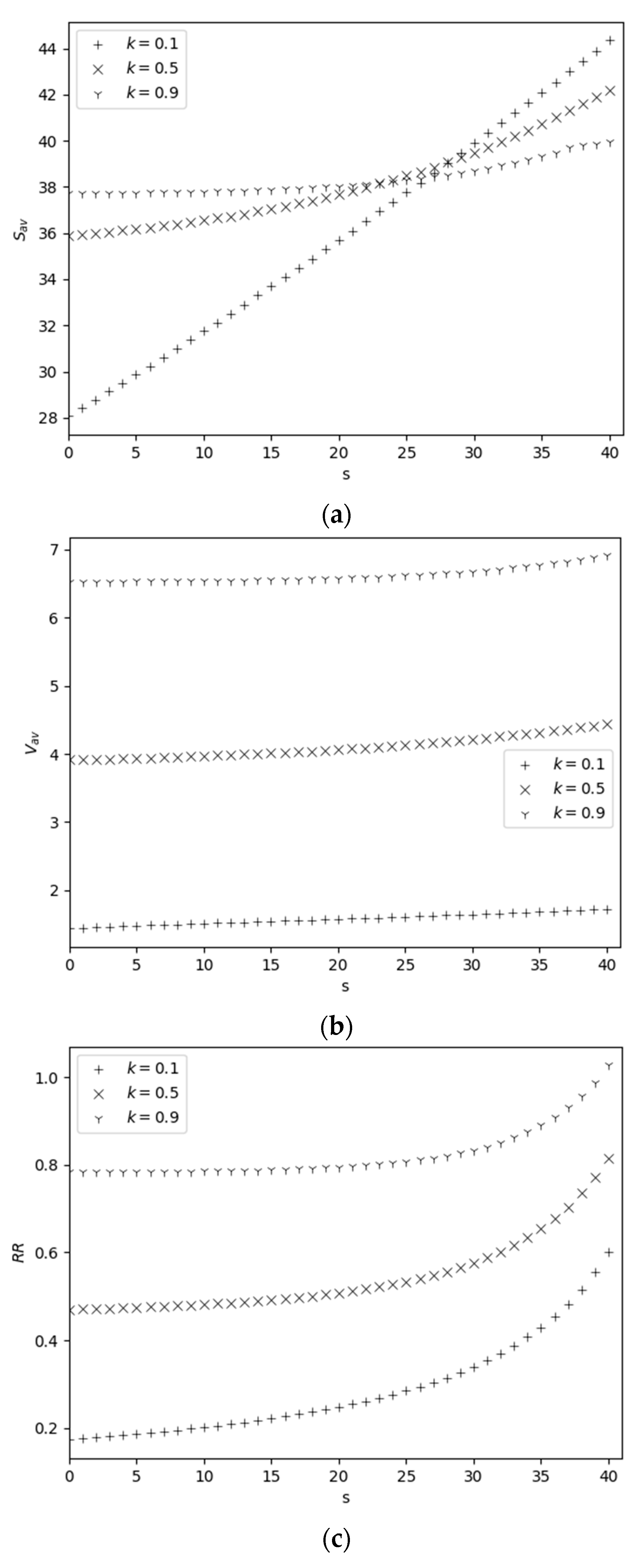
• The mean number of items in the warehouse (i.e., the average inventory level) is calculated as a mathematical expectation of the appropriate random variable and is given by the following:

  $$S_{av}={\sum }_{m=1}^{S}m{\sum }_{n=0}^{R}p\left(n,m\right) .$$

  (8)
• Similar to (8), the average order size (i.e., the average size of replenished items from external source) is calculated as a mathematical expectation of the appropriate random variable and is calculated as follows:

  $$V_{av}={\sum }_{m=S-s}^{S}m{\sum }_{n=0}^{R}p\left(n,S-m\right) .$$

  (9)
• An inventory order is placed in two cases: (1) if the inventory level drops to the re-order point $s$ after completing customer service in states $\left(n,s+1\right)\in E_{s+1}$, or (2) if catastrophes occur in the states $\left(n,m\right)\in E_m, m>0.$ Therefore, the average reorder intensity is calculated as follows:

  $$RR=\mu {\sum }_{n=1}^{R}p\left(n,s+1\right)+\kappa \left(1-{\sum }_{n=0}^{R}p\left(n,0\right)\right).$$

  (10)

The second group of performance measures includes the average length of the queue $\left(L_{av}\right)$ and loss rate of c-customers $\left(LR\right)$.

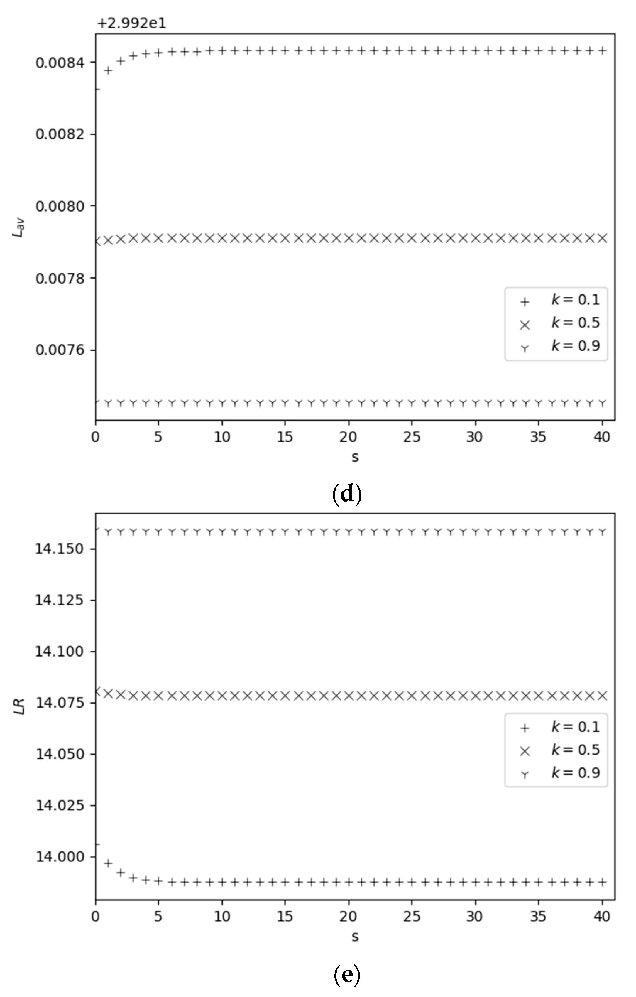
• The mean length of the queue is calculated as a mathematical expectation (an average value) of the appropriate random variable and is given by the following:

  $$L_{av}={\sum }_{n=1}^{R}n{\sum }_{m=0}^{S}p\left(n,m\right) .$$

  (11)
• Losing c-customers occurs in three cases: (1) if, at the time the c-customer arrives, the waiting room is full (with probability 1), i.e., the system is in one of the states $\left(R,m\right)\in E_m$, $m=0,1,\cdots ,S$; (2) if, at the time the c-customer arrives, the inventory level is zero and the waiting room is not full (with probability ${\phi }_2$), i.e., the system is in one of the states $\left(n,0\right)\in E_0$, $n<R;$(3) when an n-customer arrives, it displaces one c-customer. Therefore, the loss rate of c-customers is calculated as follows:

  $$LR={\mathsf{\lambda }}^{+}{\sum }_{m=0}^{S}p\left(R,m\right)+{\mathsf{\lambda }}^{+}{\phi }_2{\sum }_{n=0}^{R-1}p\left(n,0\right)+{\mathsf{\lambda }}^{-}\left(1-{\sum }_{m=0}^{S}p\left(0,m\right)\right).$$

  (12)

As mentioned above, the proposed exact approach is an effective tool for investigating the QIS model with moderate state space. Computational difficulties arise for large-scale models, in which case the development of an approximate method for determining steady-state probabilities is an urgent problem. In the next subsection, we develop an approximate method for solving this problem that can be used in cases of rare catastrophes.

3.2. An Approximate Approach

In this subsection, we derive the closed-form approximate solution for the steady-state probabilities of the investigated 2D CTMC by using a space merging approach; see [23]. This approach is highly accurate for systems with rare catastrophes, i.e., it is assumed that $\kappa \ll min\left({\lambda }^{+},{\lambda }^{-},\mu \right).$ Note that the last assumption is not extraordinary, since in the opposite case (i.e., when the rate of catastrophes is close to the rate of c-customers, the speed of their service, and the rate of n-customers), the QIS under consideration is generally not effective.

In the case where the above assumption is fulfilled, the basic requirement for an adequate application of the space-merging method is satisfied. In this case, transition rates between states in each subset $E_m$ (see (1)) are much greater than the transition rates between states from different subsets. So, in accordance with the space merging algorithm, a subset of states $E_m$ in (1) is combined into one merged state $<m>$, and the merging function in the initial state space (1) is defined as follows: $U\left(n,m\right)=<m>, \left(n,m\right)\in E$. The merged states constitute the set $\widehat{E}=\left\{<m>:m=0,1,\dots ,S\right\}.$ Then, to calculate the approximate values of steady-state probabilities, $\widehat{p}\left(m,n\right),$ we have the following formula:

$$\widehat{p}\left(n,m\right)\approx {\rho }_m\left(n\right)\pi \left(<m>\right)$$

(13)

where ${\rho }_m\left(n\right)$ denotes the probability of state $\left(n,m\right)$ within subset $E_m$ and $\pi \left(<m>\right)$ denotes the probability of merged state $<m>\in \widehat{E}$.

From relations (2), we conclude that the state probabilities ${\rho }_0\left(n\right), n=0,1,\cdots ,R$within a split model with the state space $E_0$ coincide with the distribution of a finite birth–death process in which the birth rate is ${\lambda }^{+}{\phi }_1$, while the death rate is ${\lambda }^{-}$. In the same way, from relations (2), we conclude that the state probabilities ${\rho }_m\left(n\right), m>0,n=0,1,\cdots ,R$within a split model with the state space $E_m$ are independent of $m$and coincide with the distribution of a finite birth–death process in which the birth rate is ${\lambda }^{+}$, while the death rate is ${\lambda }^{-}$. In other words, state probabilities within split models are determined as follows:

$${\rho }_m\left(n\right)=\left\{\begin{array}{cc}{\theta }^n\frac{1-\theta }{1-{\theta }^{R+1}},& m>0,n=0,1,\dots ,\mathrm{R}\\ {\theta }_0^n\frac{1-{\theta }_0}{1-{\theta }_0^{R+1}},& m=0,n=0,1,\dots ,\mathrm{R}\end{array}\right.$$

(14)

where ${\theta }_0={\mathsf{\lambda }}^{+}{\phi }_1/{\mathsf{\lambda }}^{-} \mathrm{a}\mathrm{n}\mathrm{d} \theta ={\theta }_0/{\phi }_1.$

Note 1. 

To simplify the notation, for cases $m>0$ below, the subscript $m$ is omitted in state probabilities ${\rho }_m\left(n\right).$ In cases where $\theta =1$ and/or${ \theta }_0=1$, all state probabilities ${\rho }_m\left(n\right)=1/\left(R+1\right)$ for each $n, n=0,1,\dots ,R$ and $m, m=0,1,\dots ,S$.

Let us denote the transition rate from the merged state $<m_1>$ to the merged state $<m_2>$ by $q\left(<m_1>,<m_2>\right)$. Then, taking into account relations (2) and (14), we propose the following formulas for determining these rates (all other transition rates are zero):

• Case $0\le m\le s:$

  $$q\left(<m>,<S>\right)=\mathsf{\nu }{\sum }_{n=0}^R{\rho }_m\left(n\right)=\mathsf{\nu }.$$

  (15)
• Case $m>0:$

  $$q\left(<m>,<0>\right)=\mathsf{\kappa }{\sum }_{n=0}^R{\rho }_m\left(n\right)=\mathsf{\kappa };$$

  (16)

  $$q\left(<m>,<m-1>\right)=\mu {\sum }_{n=1}^R{\rho }_m\left(n\right)=\mu \left(1-\rho \left(0\right)\right).$$

  (17)

In other words, the merged model represents a one-dimensional Markov chain in state space $\widehat{E}$ where transition rates between merged states are calculated via Formulas (15)–(17). Using the approach proposed in [11], we develop the following closed-form formulas for calculating the probabilities of merged states:

$$\pi \left(0\right)=\frac{1+bc}{1+dc},$$

(18)

$$\pi \left(1\right)=d\pi \left(0\right)-b,$$

(19)

$$\pi \left(m\right)=a_m\pi \left(1\right),2\le m\le S,$$

(20)

where the following statements are true:

$$\begin{gathered} d=\frac{\nu +\kappa }{\mu \left(1-\rho \left(0\right)\right)}, b=\frac{\kappa }{\mu \left(1-\rho \left(0\right)\right)}, \\ c={\sum }_{m=1}^S{a}_m, a_m=\left\{\begin{array}{cc}{\left(1+d\right)}^{m-1},& \mathrm{if} 1\le m\le s+1,\\ {\left(1+d\right)}^s{\left(1+b\right)}^{m-s-1},& \mathrm{if} s+1<m\le S.\end{array}\right. \end{gathered}$$

Eventually, taking into account Formulas (13), (14), and (18)–(20), we conclude that the approximate values of performance measures (8)–(12) can be calculated using the following explicit formulas:

$$S_{av}={\sum }_{m=1}^{S}m\pi \left(m\right);$$

(21)

$$V_{av}={\sum }_{m=S-s}^{S}m\pi \left(S-m\right);$$

(22)

$$RR=\mu \left(1-\rho \left(0\right)\right)\pi \left(s+1\right)+\kappa \left(1-\pi \left(0\right)\right);$$

(23)

$$L_{av}={\sum }_{n=1}^{R}n\left({\rho }_0\left(n\right)\pi \left(0\right)+\rho \left(n\right)\left(1-\pi \left(0\right)\right)\right);$$

(24)

$$\begin{gathered} LR={\lambda }^{+}{\phi }_2\pi \left(0\right)\left(1-{\rho }_0\left(0\right)\right)+{\lambda }^{+}{\rho }_0\left(R\right)\pi \left(0\right)+{\lambda }^{+}\left(1-\pi \left(0\right)\right)\rho \left(R\right)+ \\ {\lambda }^{-}\left(\pi \left(0\right)\left(1-{\rho }_0\left(0\right)\right)+\left(1-\pi \left(0\right)\right)\left(1-\rho \left(0\right)\right)\right) \end{gathered}$$

(25)

4. Numerical Experiments

Below, we demonstrate the results of numerical experiments with three objectives: (1) assess the accuracy of the proposed approximate formulas; (2) study the behavior of the performance indicators depending on the re-order point and loading parameters; and (3) solve the optimization problem.

4.1. Accuracy of the Developed Approximate Formulas

The accuracy of the proposed approximate formulas is investigated via numerical evaluations. For this purpose, exact values of the steady-state probabilities (SSP) are determined from SBE (3)–(7) for the QIS with a maximum capacity of warehouse $S=50$ and buffer size $R=30,$where the dimension of SBE is equal to 1581. The accuracy of the developed approximate formulas can be estimated using several norms, e.g., cosine similarity, Euclidean distance, Jaccard norm, etc. To be specific, here, we use a simple norm, that is, the maximum errors when calculating SSPs. Some results of numerical evaluations are shown in

Table 1. Dependence of the absolute error of the SSPs and performance measures vs. $s$; ${\lambda }^{+}=15, {\lambda }^{-}=1,\mu =2,\kappa =0.1, \nu =1,{\phi }_1=0.4$.

$\mathit{s}$	Max of Error for SSPs	Error for
		${\mathit{S}}_{\mathit{a}\mathit{v}}$	${\mathit{V}}_{\mathit{a}\mathit{v}}$	$\mathit{R}\mathit{R}$	${\mathit{L}}_{\mathit{a}\mathit{v}}$	$\mathit{L}\mathit{R}$
0	$1.17\times {10}^{-3}$	$7.01\times {10}^{-2}$	$1.12\times {10}^{-1}$	$1.23\times {10}^{-2}$	$1.41\times {10}^{-1}$	$1.54\times {10}^{-2}$
5	$1.02\times {10}^{-3}$	$6.05\times {10}^{-1}$	$1.13\times {10}^{-2}$	$1.05\times {10}^{-2}$	$1.02\times {10}^{-1}$	$1.27\times {10}^{-2}$
10	$2.15\times {10}^{-3}$	$3.11\times {10}^{-2}$	$2.29\times {10}^{-2}$	$1.91\times {10}^{-2}$	$1.17\times {10}^{-1}$	$1.36\times {10}^{-2}$
15	$8.77\times {10}^{-4}$	$4.02\times {10}^{-2}$	$3.01\times {10}^{-2}$	$5.14\times {10}^{-2}$	$1.43\times {10}^{-1}$	$1.78\times {10}^{-2}$
20	$7.01\times {10}^{-4}$	$3.18\times {10}^{-1}$	$6.08\times {10}^{-2}$	$4.02\times {10}^{-2}$	$2.01\times {10}^{-1}$	$2.15\times {10}^{-2}$
25	$3.73\times {10}^{-3}$	$5.02\times {10}^{-2}$	$7.11\times {10}^{-2}$	$2.72\times {10}^{-2}$	$2.02\times {10}^{-1}$	$3.01\times {10}^{-2}$
30	$2.16\times {10}^{-3}$	$1.08\times {10}^{-2}$	$4.33\times {10}^{-2}$	$5.05\times {10}^{-2}$	$1.04\times {10}^{-1}$	$2.02\times {10}^{-2}$
35	$2.41\times {10}^{-3}$	$3.13\times {10}^{-1}$	$1.02\times {10}^{-1}$	$1.92\times {10}^{-2}$	$1.51\times {10}^{-1}$	$1.32\times {10}^{-2}$
40	$1.24\times {10}^{-3}$	$1.02\times {10}^{-1}$	$8.12\times {10}^{-2}$	$1.82\times {10}^{-2}$	$1.11\times {10}^{-1}$	$1.03\times {10}^{-2}$
45	$3.45\times {10}^{-3}$	$1.03\times {10}^{-1}$	$2.01\times {10}^{-1}$	$1.09\times {10}^{-2}$	$1.21\times {10}^{-1}$	$1.17\times {10}^{-2}$

. In this table, along with an indication of the accuracy of calculating the SSPs, results are given that indicate the accuracy of calculating the performance measures (8)–(12). From this table, we conclude that the accuracy of the proposed approximate formulas for calculating SSPs and performance indicators is high for engineering applications. From this table, it is also clear that the accuracy of calculating the SSPs is greater than the accuracy of calculating performance indicators. This was to be expected, since the performance indicators are calculated through SSPs using operations of multiplication by large numbers; see Formulas (8)–(12) and (21)–(25). We conducted a large number of experiments and summarize only a small part of them here. An interesting result of these experiments is that the larger the system size (i.e., increasing S and R), the higher the accuracy of the approximate results obtained.

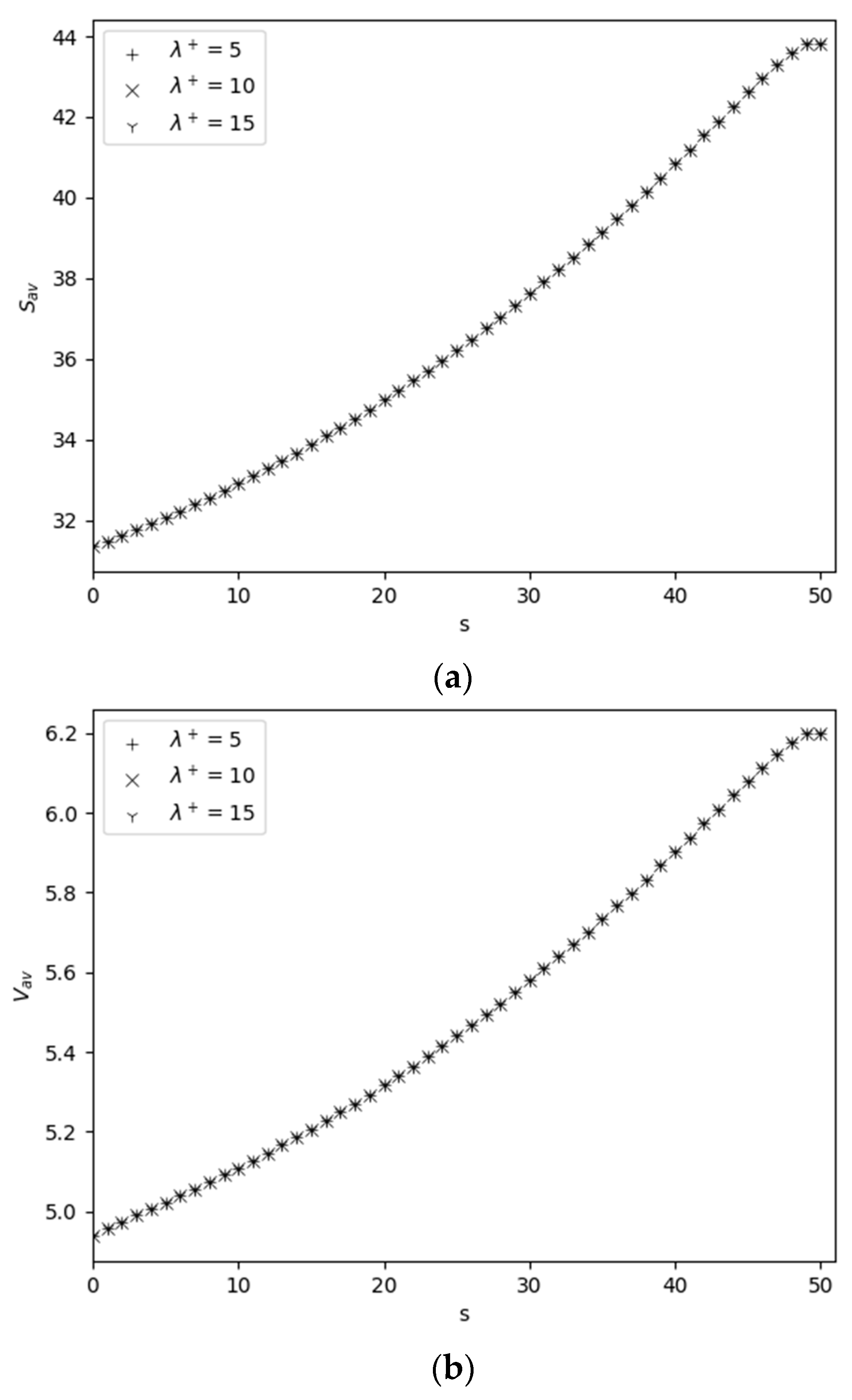
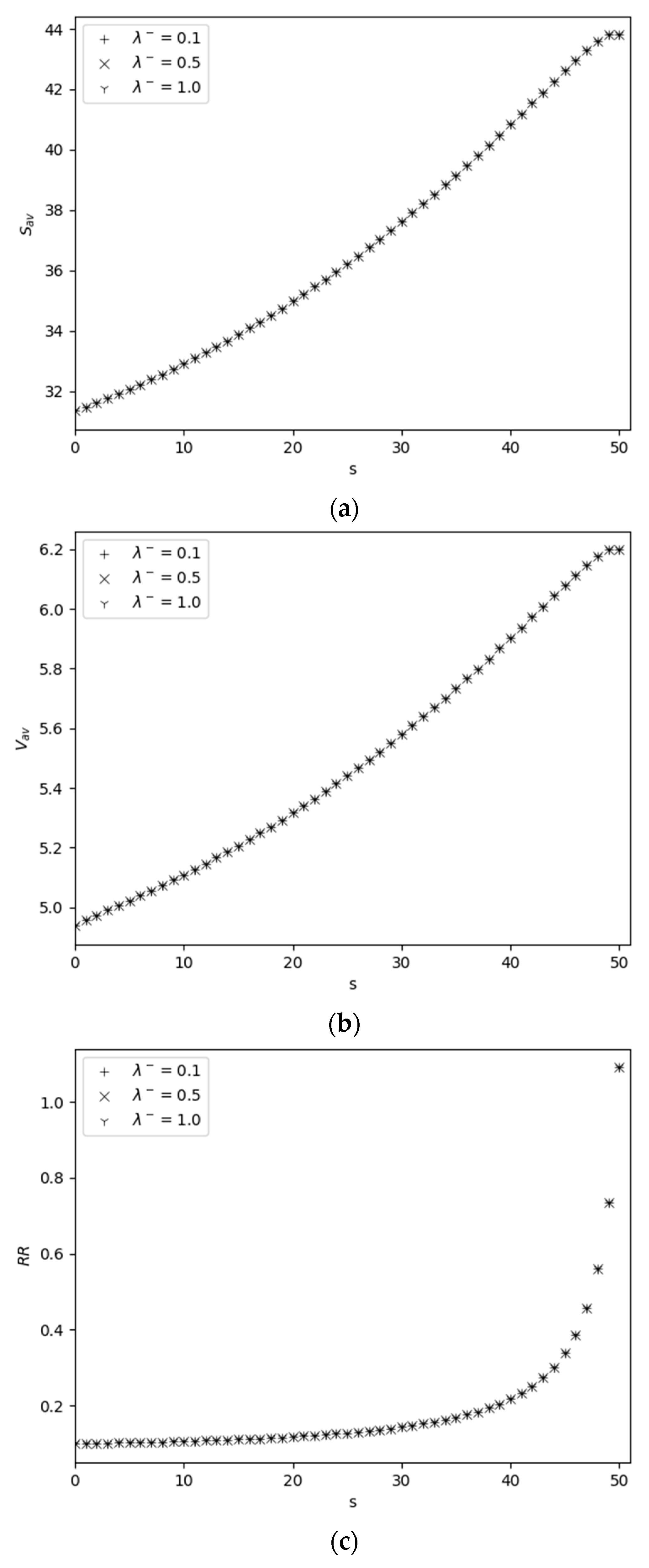
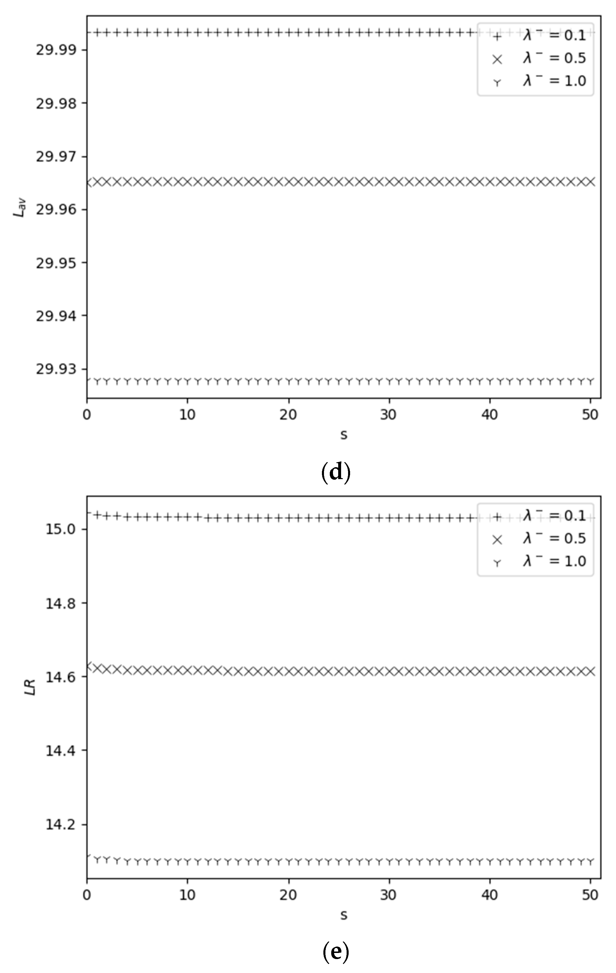
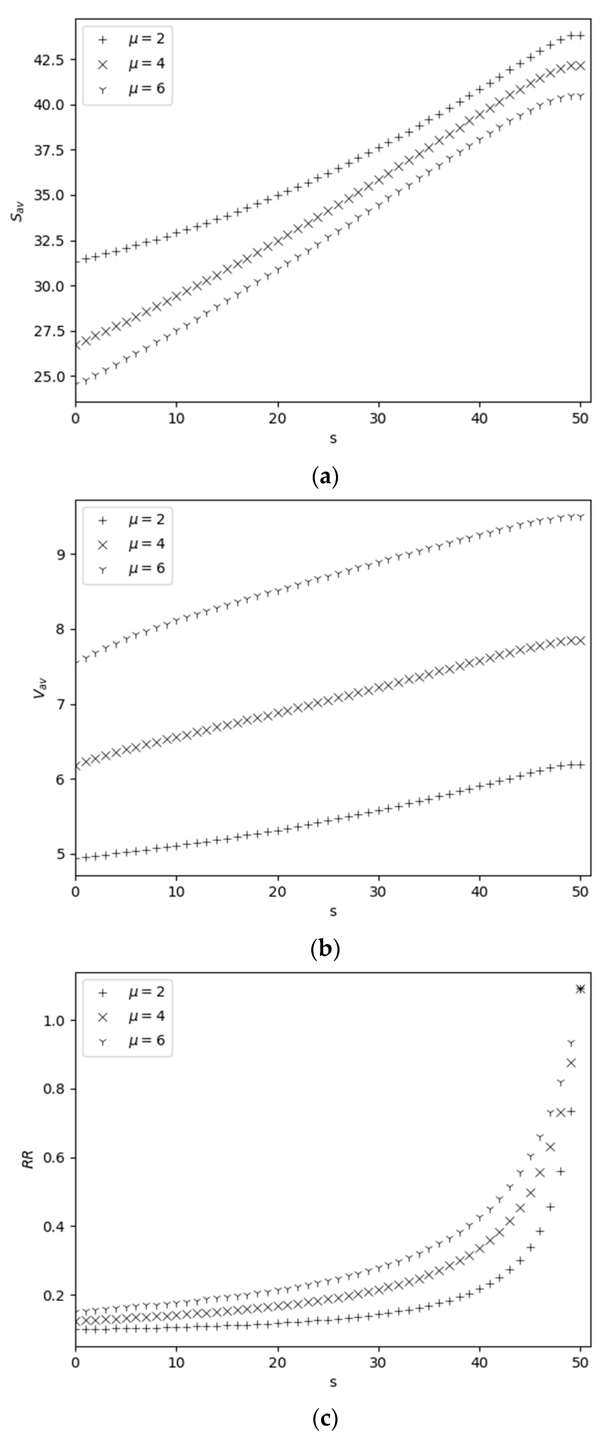
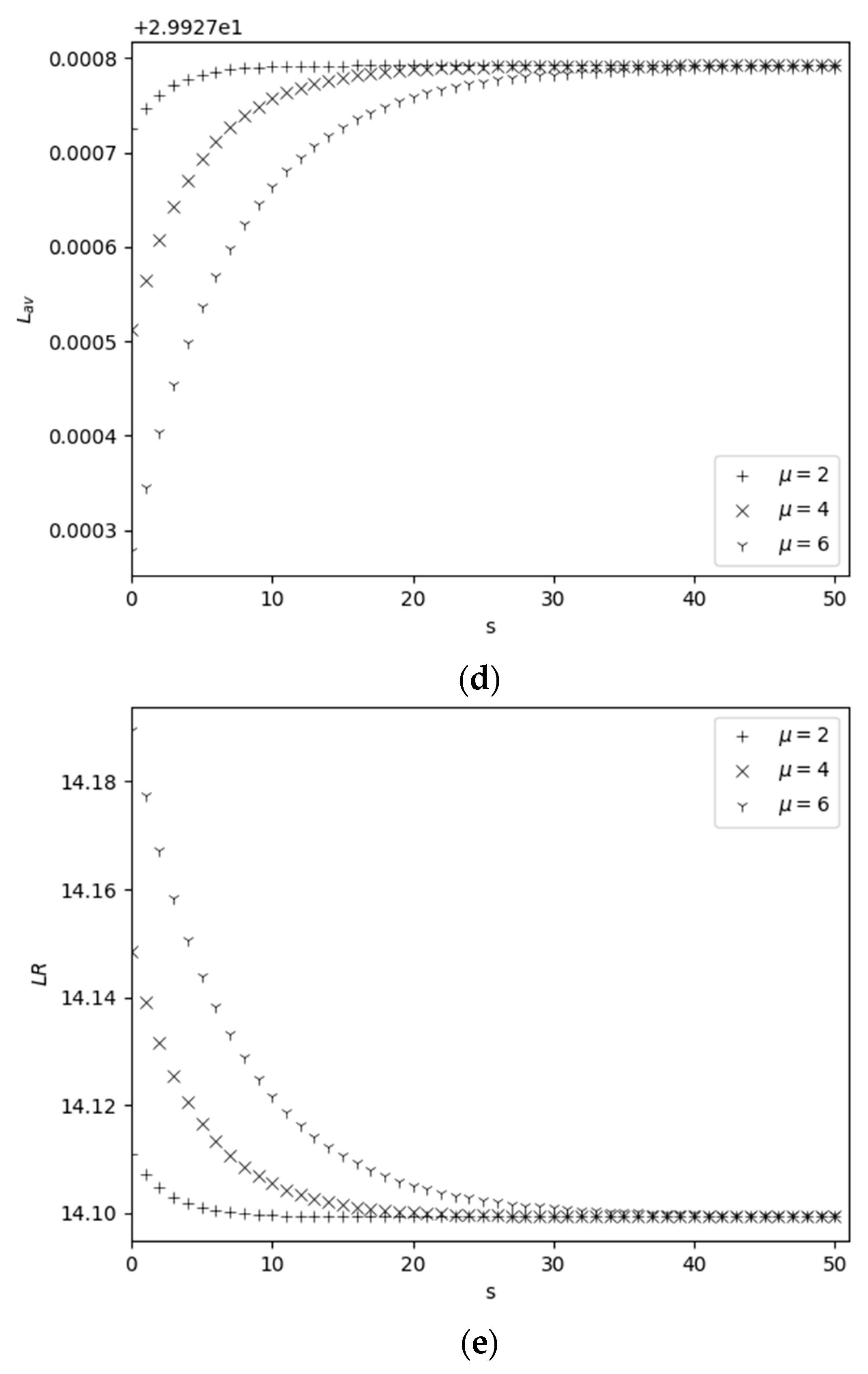
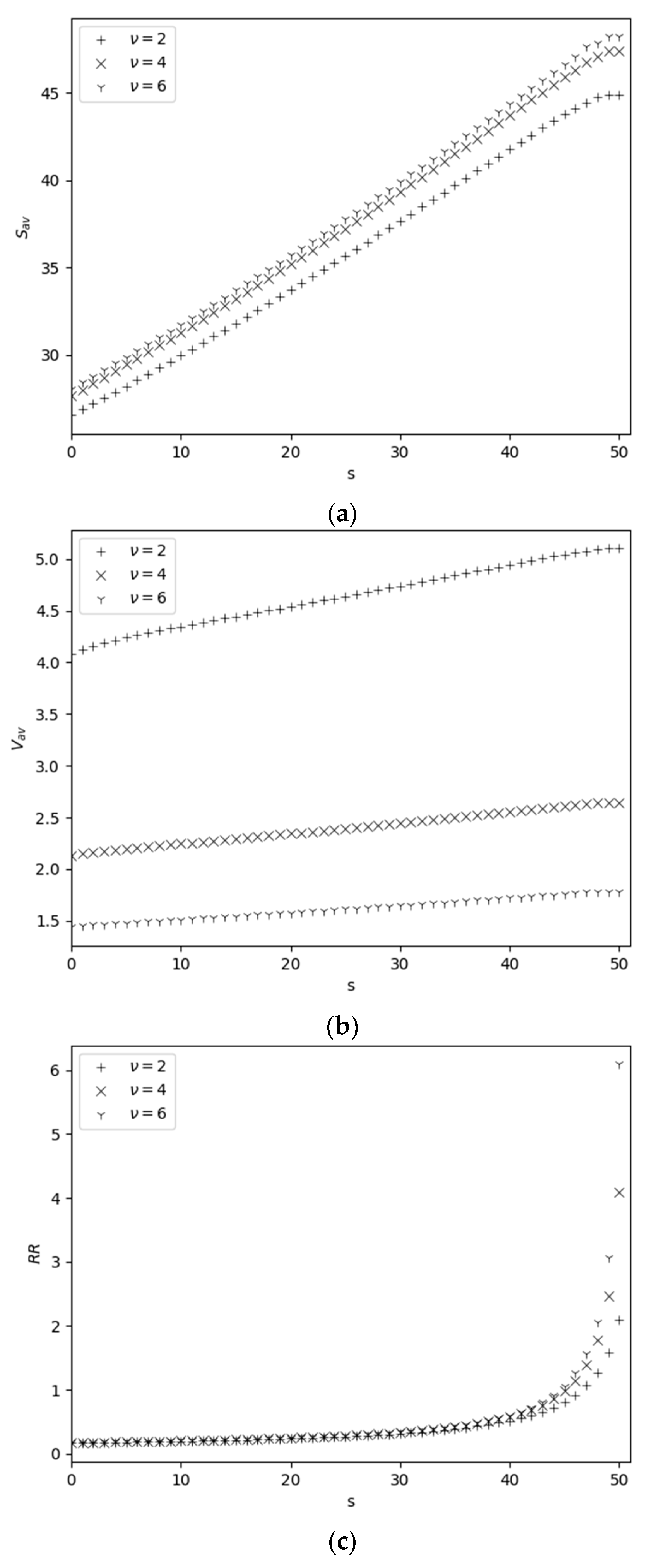
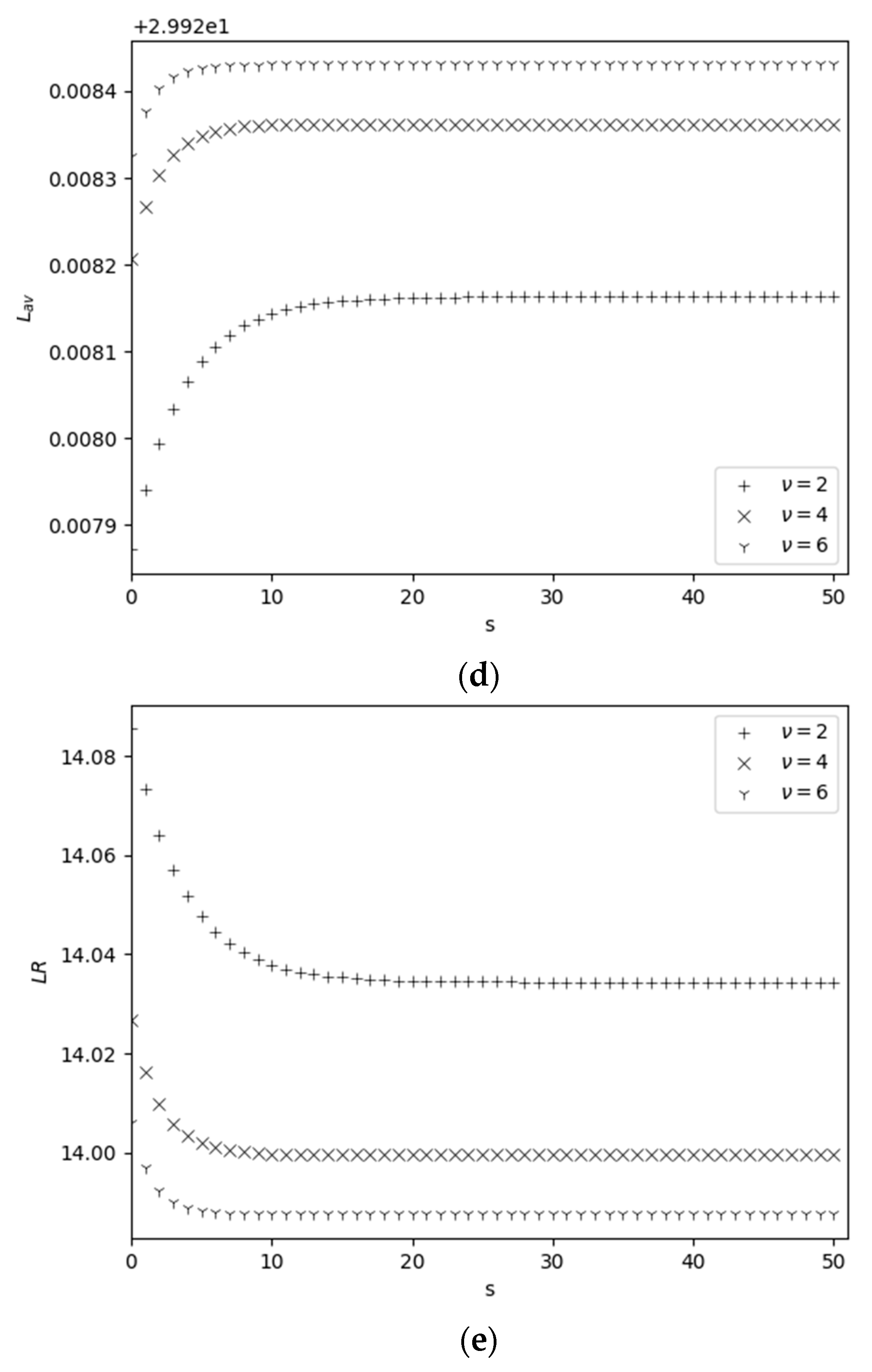
4.2. Behavior of Performance Measures versus Reorder Point

Performance measures are computed and numerically evaluated for different sets of values for the loading parameters and the reorder point. In all experiments, the values of the following parameters are fixed: $S=50, N=30, { \phi }_1=0.4, \kappa =0.1.$ So, Figure 1 shows the dependence of performance indicators on reorder point $s$ for the three different values of ${\lambda }^{+}$, where $\mu =2, \nu ={\lambda }^{-}=1.$From these plots, we conclude that inventory-related performance measures are almost independent of the rate of c-customers but significantly dependent on the reorder point, see Figure 1a–c. Note that all inventory-related performance measures are increasing functions versus reorder points. Measure$S_{av}$ is an increasing function versus $s$, and this fact was expected; see Figure 1a. At first glance, the increase in $V_{av}$ versus $s$ seems unexpected; see Figure 1b. However, this fact has the following explanation: as $s$ increases, the reorder rate increases (see Figure 1c), and as a result, the average order size increases. The $RR$ is an increasing function with respect to $s$ because as $s$ increases, the probability that the inventory level is positive also increases and, hence, $RR$ becomes an increasing function; see Formula (10) as well. For the selected data, the rate of its increase becomes very high at large (possible) values of the reorder point, see Figure 1c. In contrast, the queuing-related performance measures are almost independent of the reorder point, see Figure 1d,e. For selected initial data, the mean number of consumer customers in systems $\left(L_{av}\right)$for all values of ${\lambda }^{+}$ are very close to the buffer size ($R=30$); see Figure 1d. Therefore, the loss rate $\left(LR\right)$ is very close to ${\lambda }^{+}$; see Figure 1e.

The dependence of performance measures on $s$ and ${\lambda }^{-}$ is shown in Figure 2, where ${\lambda }^{+}=15,\mu =2, \mathrm{a}\mathrm{n}\mathrm{d} \nu =1.$ It is interesting to note that here, the behavior of the measures, including the absolute values of the inventory-related performance measures (see Figure 2a–c), is the same as in Figure 1a–c. From Figure 2d, we conclude that $L_{av}$ is almost independent of $s$ and the rate of its decrease versus ${\lambda }^{-}$ is very small, i.e., increasing ${\lambda }^{-}$ even by ten times leads to a change in the value of $L_{av}$ in the second digit after the decimal point. Similarly, from Figure 2e, we conclude that $LR$ is also almost independent of $s$, but, here, the rate of its decrease compared to ${\lambda }^{-}$ is noticeable.

The dependence of performance measures on $s$ and $\mu$ is shown in Figure 3, where ${\lambda }^{+}=15 \mathrm{a}\mathrm{n}\mathrm{d} \nu ={\lambda }^{-}=1$. An increase in $S_{av}$ with respect to $s$ is obvious, since when $s$ increases, the rate of filling the warehouse to its maximum size also increases; see Figure 3a; on the other hand, $S_{av}$ is a decreasing function versus $\mu$ because as μ increases, the rate of inventory sales increases. $S_{av}$ decreases with respect to $\mu$, therefore, $V_{av}$ increases with respect to $\mu$; see Figure 3b; an increase in $s$ leads to increasing the probability that the inventory level drops to zero due to catastrophes, i.e., the average order size is also an increasing function versus $s$. Measure $RR$ is an increasing function with respect to $s$, since increasing $s$ leads to increasing the probability that the inventory level is positive, i.e., the rate of replenishment of stocks due to catastrophes also increases; see Figure 3c; this measure is also an increasing function with respect to $\mu$, since an increase in $\mu$ leads to an increase in the probability that the inventory level drops to the re-order point $s$, i.e., the rate of replenishment increases (see Formula (9) also). From Figure 3d, we conclude that $L_{av}$ is an increasing function versus $s$ and a decreasing function versus $\mu$. And, for large values of $s$, i.e., $s>25,$ the value of $L_{av}$ is practically independent of $\mu$. These facts are expected. Measure $LR$ is a decreasing function versus both $s$ and $\mu$; see Figure 3e. The decrease in this function with respect to $s$ is obvious, but its decrease relative to $\mu$ is not evident at first glance. The last fact has the following explanation: an increase in $\mu$ leads to an increase in the probability that the inventory level is zero, i.e., the loss probability of arriving consumer customers also increases, and, hence, the measure $LR$ becomes an increasing function. However, the rate of increasing $LR$ versus $\mu$ is very small, i.e., increasing $\mu$ even by three times leads to a change in the value of $LR$ in the second digit after the decimal point.

The dependence of performance measures on $s$ and ν is shown in Figure 4, where ${\lambda }^{+}=15,\mu =2,{\lambda }^{-}=1$. The measure $S_{av}$ increases both in $s$ and ν, see Figure 4a. Indeed, an increase in $s$ and ν leads to an increase in the rate of filling the warehouse to its maximum size. Measure $V_{av}$ is increasing versus $s$, while it is a decreasing function versus ν. Here $V_{av}$ is decreasing versus ν, since $S_{av}$ is an increasing function with respect to ν; see Figure 4b; the increase in $V_{av}$ with respect to $s$ is explained as above, i.e., as s increases, the probability that the inventory levels fall to zero due to catastrophes also increases, so the average order size is also an increasing function versus $s$. Measure $RR$ is an increasing one with respect to both $s$ and ν, since an increase in both $s$ and ν leads to an increase in the probability that the inventory level is positive; hence, the rate of replenishment of inventory due to catastrophes also increases; see Figure 4c. From Figure 4d, we conclude that the $L_{av}$ is almost constant (does not decrease) depending on $s$ and ν; only for small values of $s$, i.e., s < 10, we observe insignificant differences between the values of $L_{av}$ for different values of ν. Measure $LR$ is a decreasing function versus both $s$ and ν, see Figure 4e. This behavior of this measure is expected, since an increase in both $s$ and ν leads to an increase in the average inventory level and, as a result, to a decrease in $LR$.

We also numerically studied the impact of catastrophe rate on system performance measures (see Figure 5), where $\mathit{S}=\mathbf{50},\mathit{R}=\mathbf{30},{\lambda }^{+}=\mathbf{15},{\mathsf{\lambda }}^{-}=\mathbf{1},\mathsf{\mu }=\mathbf{2},\mathsf{\nu }=\mathbf{1},\mathrm{a}\mathrm{n}\mathrm{d} {\mathsf{\phi }}_{\mathbf{1}}=\mathbf{0.4}$. When $\mathit{s}$ changes from zero and 28, the average inventory levels $\left({\mathit{S}}_{\mathit{a}\mathit{v}}\right)$ are higher at higher catastrophe intensity values, and for $\mathit{s}$ greater than 28, the opposite picture is observed; see Figure 5a. At first glance, such behavior of function ${\mathit{S}}_{\mathit{a}\mathit{v}}$ is unexpected, since the higher the intensity of catastrophes, the lower the average level of inventory should be. However, this is only so at first glance. At a low intensity of catastrophe, the available inventories of a high level are used by c-customers, and as a result, the average inventory level turns out to be lower than at a high intensity of catastrophe. It is important to note that these explanations apply only to selected input parameter values, i.e., with other values of the input parameters, observations of a different picture are possible. In other words, the behavior of ${\mathit{S}}_{\mathit{a}\mathit{v}}$ versus the intensity of catastrophes significantly depends on the values of other parameters. Here ${\mathit{V}}_{\mathit{a}\mathit{v}}$ is increasing function versus both $\mathit{s}$ and $\kappa$, and its value significantly depends on the value of catastrophe intensity, but very slowly changed versus $\mathit{s}$; see Figure 5b. The behavior of RR depending on $\mathit{s}$ and κ is similar to ${\mathit{V}}_{\mathit{a}\mathit{v}}$, but here, the growth rate of RR is moderate in both parameters; see Figure 5c. Note that for selected values of initial parameters, both queuing-related performance measures, ${\mathit{L}}_{\mathit{a}\mathit{v}}$ and $\mathit{L}\mathit{R},$ are practically independent of κ; see Figure 5d,e.

4.3. Optimization Problem

The third goal of performing numerical experiments is solving the optimization problem. To be specific, here, the minimization of Expected Total Cost (ETC) is considered. In this problem, it is assumed that all load parameters and structural parameters of the QIS are fixed, and the only controllable parameter is the reorder point. Similar to Melikov et al. (2023) [11], ETC is defined as follows:

$$ETC\left(s\right)=\left(K+c_r·V_{av}\right)·RR+c_h·S_{av}+c_{ps}·\mathsf{\kappa }{·S}_{av}+c_l·LR+c_w{·L}_{av}$$

(26)

where $K$ is the fixed price of one order, $c_r$ is the unit price of the order size, $c_h$ is the unit item storage price per unit of time, $c_{ps}$ is the price of unit item destruction, $c_l$ is the cost for a single consumer customer loss, and $c_w$ is the price per unit time of delay for a single consumer customer.

The problem is to find a value (optimal) of $s$ that minimizes (26). For any values of initial parameters, this problem has a solution, since the admissible set for values of $s$ is finite and discrete, i.e., $0\le s\le S-1.$ Coefficients in (26) for the hypothetical model are selected as $K=10,c_r=15,c_h=10,c_l=450,c_w=400, \mathrm{a}\mathrm{n}\mathrm{d} c_{ps}=15$. Some results of the minimization of (26) are demonstrated in

Table 2. Optimization problem results.

$\mathit{S}$	${\mathit{S}}_{\mathit{a}\mathit{v}}$	${\mathit{V}}_{\mathit{a}\mathit{v}}$	$\mathit{R}\mathit{R}$	${\mathit{L}}_{\mathit{a}\mathit{v}}$	$\mathit{L}\mathit{R}$	${\mathit{E}\mathit{T}\mathit{C}}^{\mathbf{*}}$
50	28.07176	1.439081	0.172690	29.92832	13.98755	18,981.34
55	31.23721	1.493466	0.162924	29.92834	13.98755	19,059.21
60	34.46487	1.548604	0.154860	29.92835	13.98755	19,138.86
65	37.75379	1.604545	0.148112	29.92836	13.98755	19,220.23
70	41.10292	1.661316	0.142398	29.92837	13.98755	19,303.25

. Here, we assume that $N=30, {\phi }_1=0.4, {\lambda }^{+}=15, {\lambda }^{-}=1, \kappa =0.1,\mu =2, \mathrm{a}\mathrm{n}\mathrm{d} \nu =1.$ The optimal solution for indicated values of $S$ is $s^{*}=0$. For completeness, Table 2 shows the values of the performance measures in the optimal solution, as well as the minimum value of the expected total cost that is denoted by ${ETC}^{*}.$

5. Conclusions

The model of QIS with one server, catastrophes in the warehouse, and a finite waiting room for consumer customers was proposed. When a catastrophe occurs, the entire inventory, including the items that were in the status of release to the consumer, are instantly destroyed. However, catastrophes do not push out consumers. It is assumed that if the inventory level upon arrival of the consumer customer is zero, then, in accordance with the Bernoulli trials, it either joined the buffer of infinite size or left the system unserved. In the system, the “Up to S” replenishment policy is applied. In addition to c-customers, negative customers also enter the system. When a negative customer arrives, one of the consumers, if any, is pushed out. The mathematical model of the investigated QIS is constructed as a two-dimensional continuous-time Markov chain. Both exact and approximate methods for calculating steady-state probabilities and performance indicators of the QIS under study are proposed. The exact method is based on balance equations, while the approximate method is based on the space merging approach. It is noted that the proposed approximate method has high accuracy in the case of rare catastrophes. Closed-form formulas for calculating the performance indicators were proposed. The results of numerical evaluations are demonstrated.

For brevity, only the QIS model with the “Up to S” replenishment policy is considered here. A direction for further research is to explore a similar model with other commonly used replenishment policies, e.g., $\left(s, Q\right), Q=S-s>s,$ $\left(S-1,S\right)$or a randomized replenishment policy. These studies will make it possible to compare the performance of various replenishment policies, and, thus, choose the optimal (in a certain sense) replenishment policy. Another direction for further research should be the study of similar models with MAP flows of c-customers and/or n-customers, as well as with the PH distribution of service times for c-customers and/or lead times.

References

1. Chakravarthy, S.R. A catastrophic queueing model with delayed action. Appl. Math. Model. 2017, 46, 631–649. [Google Scholar] [CrossRef]
2. Kumar, D.; Singh, B.G. Transient Solution of a Two Homogeneous Servers Markovian Queueing System with Environmental, Catastrophic and Restoration Effects. Int. J. Math. Stat. Stud. 2024, 12, 45–53. [Google Scholar] [CrossRef]
3. Demircioglu, M.; Bruneel, H.; Wittevrongel, S. Analysis of a Discrete-Time Queueing Model with Disasters. Mathematics 2021, 9, 3283. [Google Scholar] [CrossRef]
4. Kumar, B.K.; Arivudainambi, D. Transient solution of an M/M/1 queue with catastrophes. Comput. Math. Appl. 2000, 40, 1233–1240. [Google Scholar] [CrossRef]
5. Jain, N.K.; Rakesh, K. Transient solution of a catastrophic-cum-restorative queuing problem with correlated arrivals and variable service capacity. Int. J. Inform. Manag. Sci. 2007, 18, 461–465. [Google Scholar]
6. Jain, N.K.; Singh, B.G. A queue with varying catastrophic intensity. Int. J. Comput. Appl. Math 2010, 5, 41–46. [Google Scholar]
7. Singh, B.G.; Niwas, B.R. Time-dependent analysis of a queueing system incorporating the effect of environment, catastrophe, and restoration. J. Reliab. Stat. Stud. 2015, 8, 29–40. [Google Scholar]
8. Krishnamoorthy, A.; Joshua, A.N.; Mathew, A.P. The k-out-of-n: G System Viewed as a Multi-Server Queue. Mathematics 2024, 12, 210. [Google Scholar] [CrossRef]
9. Rykov, V.; Kochueva, O.; Farkhadov, M. Preventive Maintenance of a k-out-of-n System with Applications in Subsea Pipeline Monitoring. J. Mar. Sci. Eng. 2021, 9, 85. [Google Scholar] [CrossRef]
10. Melikov, A.; Mirzayev, R.R.; Nair, S.S. Numerical investigation of double source queuing-inventory systems with destructive customers. J. Comput. Syst. Sci. Int. 2022, 61, 581–598. [Google Scholar] [CrossRef]
11. Melikov, A.; Poladova, L.; Edayapurath, S.; Sztrik, J. Single-Server Queuing-Inventory Systems with Negative Customers and Catastrophes in the Warehouse. Mathematics 2023, 11, 2380. [Google Scholar] [CrossRef]
12. Neuts, M.F. Matrix-Geometric Solutions in Stochastic Models: An Algorithmic Approach; The Johns Hopkins University Press: Baltimore, MD, USA, 1981. [Google Scholar]
13. Chakravarthy, S.R. Introduction to Matrix-Analytic Methods in Queues 1—Basics; John Wiley & Sons, Inc.: London, UK, 2022; Volume 1. [Google Scholar]
14. Chakravarthy, S.R. Introduction to Matrix-Analytic Methods in Queues 2—Queues and Simulation; John Wiley & Sons, Inc.: London, UK, 2022; Volume 2. [Google Scholar]
15. Dudin, A.N.; Klimenok, V.I.; Vishnevsky, V.M. The Theory of Queueing Systems with Correlated Flows; Springer: Basel, Switzerland, 2020. [Google Scholar]
16. Amirthakodi, M.; Sivakumar, B. An inventory system with service facility and feedback customers. Int. J. Ind. Syst. Eng. 2019, 33, 374–411. [Google Scholar] [CrossRef]
17. Amirthakodi, M.; Sivakumar, B. An inventory system with a service facility and finite orbit size for feedback customers. OPSEARCH 2015, 52, 225–255. [Google Scholar] [CrossRef]
18. Amirthakodi, M.; Radhamani, V.; Sivakumar, B. A perishable inventory system with service facility and feedback customers. Ann Oper Res. 2015, 233, 25–55. [Google Scholar] [CrossRef]
19. Sivakumar, B.; Elango, C.; Arivarignan, G. A Perishable Inventory System with Service Facilities and Batch Markovian Demands. Int. J. Pure Appl. Math. 2006, 32, 33–49. [Google Scholar]
20. Devi, P.C.; Sivakumar, B.; Krishnamoorthy, A. Optimal Control Policy of an Inventory System with Postponed Demand. RAIRO-Oper. Res. 2016, 50, 145–155. [Google Scholar] [CrossRef]
21. Varghese, D.T.; Shajin, D. State Dependent Admission of Demands in a Finite Storage System. Int. J. Pure Appl. Math. 2018, 118, 917–922. [Google Scholar]
22. Jenifer, J.S.A.; Sangeetha, N.; Sivakumar, B. Optimal Control of Service Parameter for a Perishable Inventory System with Service Facility, Postponed Demands and Finite Waiting Hall. Int. J. Inform. Manag. Sci. 2014, 25, 349–370. [Google Scholar]
23. Melikov, A.; Mirzayev, R.R.; Sztrik, J. Double Sources QIS with Finite Waiting Room and Destructible Stocks. Mathematics 2023, 11, 226. [Google Scholar] [CrossRef]
Figure 1. Dependency of performance measures on s for different λ + .
Mathematics 12 00906 g001aMathematics 12 00906 g001b
Figure 2. Dependency of performance measures on s for different λ .
Mathematics 12 00906 g002aMathematics 12 00906 g002b
Figure 3. Dependency of performance measures on s for different μ .
Mathematics 12 00906 g003aMathematics 12 00906 g003b
Figure 4. Dependency of performance measures on s for different ν .
Mathematics 12 00906 g004aMathematics 12 00906 g004b
Figure 5. Dependency of performance measures on s for different κ.
Mathematics 12 00906 g005aMathematics 12 00906 g005b