The Constrained 2-Maxian Problem on Cycles

Abstract

This paper deals with p-maxian problem on cycles with an upper bound on the distances of all facilities. We consider the case of $p=2$ and show that, in the worst case, the optimal solution contains at least one vertex of the underlying cycle, which helps to develop an efficient algorithm to solve the constrained 2-maxian problem. Based on this property, we develop a linear time algorithm for the constrained 2-maxian problem on a cycle. We also discuss the relations between the constrained and unconstrained 2-maxian problems on which the underlying graphs are cycles.

1. Introduction

Facility location theory deals with the problems of planning new optimal facilities in a network of existing customers, playing an important role in operation research due to its theoretical and practical contributions. The median and center location problems are the two most important models in classical facility location theory. The aim of a median problem is to find one or several facilities to minimize the total weighted distance from customers to the facilities. Furthermore, the goal of the center problem is to locate new facilities such that the maximum weighted distance from customers to the facilities is minimized.

Since the median and center problems on general graphs are $NP$-hard, there is significant interest in cases where such a problem can be solved in polynomial time. Goldman [1] showed that the 1-median problem on trees can be solved in linear time. For the 2-median problem on trees, Gavish and Sridhar presented [2] an $O(nlogn)$ time algorithm. Tamir [3] studied the p-median problem on trees and showed that the problem can be solved in $O(p{n}^2)$ time. Burkard and Krarup [4] designed a linear time algorithm for the pos/neg-weighted 1-median problem on a cactus, and showed that the 2-median problem on cactus graphs can be solved in $O(n^2)$ time. For the model of center problems, Handler [5] presented a linear time algorithm for the 1-center problem on trees. For the p-center problem on trees, Wang and Zhang [6] presented an $O(nlogn)$ time algorithm. Lan [7] showed that the 1-center problem on a cactus graph can be solved in linear time. For the weighted 2-center problem on cactus graphs, Moshe et al. [8] devised an $O(n{logn}^3)$ time algorithm for the continuous version and showed that the discrete version is solvable in $O(n{logn}^2)$ time.

In recent years, the obnoxious facility location problem has been studied extensively, where some facilities are to be placed as far away as possible from the customers. These models are applied when locating undesirable facilities, for example, garbage dumps, airports, and chemical plants, to mention a few. For a survey of obnoxious location problems, we refer to Krarup et al. [9] and Tamir [10]. If the aim is to maximize the total maximum weighted distances from all customers to p new facilities, the corresponding problem is the so-called p-maxian problem. The p-maxian problem was first considered by Burkard et al. [11], who showed that the problem could be solved in linear time. Kang and Cheng [12] presented a linear time algorithm for the p-maxian problem on block graphs, where each block graph is a super class of tree graphs. Furthermore, the p-maxian problem on interval graphs was solved in linear time by Cheng and Kang [13]. For the 2-maxian problem on cactus graphs, Kang et al. [14] devised a quadratic time algorithm, where any two cycles in the graph have at most one vertex in common.

In real-life situations, the maximum distances between new facilities are often limited within a given bound. For instance, surveillance cameras of a residential district must be located in such a way that they are close enough for full coverage and nucleic acid collecting sites are located close enough for convenience. Considering such a limitation, the aim of the p-maxian problem is to locate p facilities such that they are close enough for inter-connection or cooperation. Nguyen et al. [15] were the first to consider the p-maxian problem with a distance constraint, and they showed that the 2-maxian problem on trees is solvable in linear time. Motivated by this paper, we consider the p-maxian problem on cycles with bounds on the maximum distances between facilities. We organize the paper in the following sections. Section 2 defines the p-maxian problem with distance constraints and gives the important properties of the 2-maxian problem as well. In Section 3, we develop a linear time algorithm for the constrained 2-maxian problem on cycles. Section 4 presents a brief conclusion to this paper.

2. Problem Definition and Properties

Let $C=(V,E)$ be a cycle of sequence $(v_1,v_2,\dots ,v_n,v_{n+1}=v_1)$ of n distinct vertices supplemented by $v_{n+1}=v_1$, such that $(v_i,v_{i+1})$ is an edge of C, $i=1,2,\dots ,n$, where all vertices are numbered in a clockwise way. Each vertex $v_i\in V$ has a non-negative weight $w_i$ and each edge $e\in E$ has a non-negative length $\ell (e)$. The length of C is denoted by $\ell (C):={\sum }_{e\in E}\ell (e)$. A point x on C may either be a vertex or may lie on an edge of C; the set of all points of C is denoted by $X(C)$. For any two points $x,y$ of $X(C)$, the length of the shortest path from x to y is denoted by $d(x,y)$, and $d^c(x,y)$ denotes the length of the path from x to y in a clockwise direction. It is easy to see that $d(x,y)=d^c(x,y)$ or $d(x,y)+d^c(x,y)=\ell (C)$ holds for any two points $x,y$ of $X(C)$.

In a p-maxian problem on the cycle graph C, the aim is to find p points of $X(C)$, say $X:=\{x_1,x_2,\dots ,x_p\}$, such that the following objective function is maximized:

$$\begin{array}{c}\hfill F(X):=\sum _{i=1}^n{w}_i·\underset{j=1,2,\dots ,p}{max}d(v_i,x_j),\end{array}$$

(1)

where the point set $X\subseteq X(C)$ that maximizes (1) is called the p-maxian of C.

In this paper, we assume that the maximum distance between facilities does not exceed a given bound $\mathcal{U}\le \frac{\ell (C)}{2}$. Then, the p-maxian problem on C with a distance constraint of $\mathcal{U}$ (constrained p-maxian problem) can be formulated as the following optimization model:

$$\begin{array}{c}\hfill maxF(X):=\sum _{i=1}^n{w}_i·\underset{j=1,2,\dots ,p}{max}d(v_i,x_j)\end{array}$$

(2)

$$\begin{array}{c}\hfill \mathrm{s}.\mathrm{t}.d(v_i,x_j)\le \mathcal{U},i=1,2,\dots ,n;j=1,2,\dots ,p,\end{array}$$

(3)

where the set $X\subseteq X(C)$ that fulfills (2) and (3) is called the constrained p-maxian of C.

For the case of $p=2$, the corresponding constrained 2-maxian problem on a cycle C is to find two points $\{x_1,x_2\}\subseteq X(C)$, which maximizes the following equation:

$$\begin{array}{c}\hfill F(x_1,x_2):=\sum _{i=1}^n{w}_i·max\{d(v_i,x_1),d(v_i,x_2)\},\end{array}$$

with the distance constraint $d(x_1,x_2)\le \mathcal{U}$.

For an unconstrained 2-maxian problem on a modified cycle, the so-called vertex optimality property asserts that the problem has an optimal solution at the vertices [14]. However, this property does not apply in our problem. For example, for the graph in Figure 1, we find

$$F(m_1=v_1,m_2)=20.5,$$

where $m_1$ is a vertex, $m_2$ is not a vertex but is the inner point of the edge $(v_2,v_3)$ with $d(m_1,m_2)\le \mathcal{U}=\frac{3}{2}$, and $\{m_1,m_2\}$ is the unique solution to the constrained 2-maxian problem. In the following, we will give an important result for the constrained 2-maxian problem on a cycle C, which characterizes the point $x\in X(C)$ that may appear in an optimal solution of the problem.

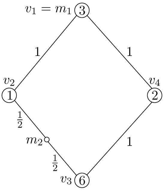
Figure 1. Vertex optimality does not hold any more.

Theorem 1. 

There exists an optimal solution $X^{*}=\{x_1,x_2\}$ of the constrained 2-maxian problem on C, such that one of the following statements holds for $x_1$ and $x_2$:

• $x_1\in V$ and $x_2\in V$.
• $x_1\in V$ and $x_2$ lies on the interior of an edge with the property of $d(x_1,x_2)=\mathcal{U}$.

Proof. 

Let $X^{*}=\{x_1,x_2\}$ be an optimal solution of the constrained 2-maxian problem on C. Suppose that $X^{*}$ is contradicting both statements 1 and 2. Obviously, there exists at least one interior point of some edge. Assume that $x_1$ is not a vertex and lies on the edge $(v_r,v_{r+1})$, and that $x_2$ lies on the edge $(v_s,v_{s+1})$ or coincides with s. Moreover, we assume that $r<s$ and $d(x_1,x_2)=d^c(x_1,x_2)\le \mathcal{U}$. For the point $x_1$, we define the following sets:

$$V_1:=\{v_i\in V|d(x_1,v_i)>d(x_2,v_i)\},$$

$$V_1^1:=\{v_i\in V_1|d(x_1,v_i)=d(x_1,v_{r+1})+d^c(v_{r+1},v_i)\},$$

$$V_1^2:=\{v_i\in V_1|d(x_1,v_i)=d(x_1,v_r)+d^c(v_i,v_r)\}.$$

For the point $x_2$, we define the sets $V_2$, $V_2^1$ and $V_2^2$ similarly. Note that all facilities of $V_1$ and $V_2$ are served by $x_1$ and $x_2$, respectively, which is denoted by $V_3=V\backslash (V_1\cup V_2)$. Note that if $V_3$ is nonempty, then all vertices of $V_3$ could be served by $x_1$ as well as by $x_2$. Without a loss of generality, we assume that $V_3=\{v_{k_1},v_{k_2}\}$ and $k_1<k_2$.

For the edge $e_r=(v_r,v_{r+1})$, we consider a function $f:[0,\ell (e_r)]\to \mathcal{R}$ depending on t, where $t=0$ corresponds to vertex $v_r$ and $t=\ell (e_r)$ corresponds to vertex $v_{r+1}$. Moreover, the interior point x on the edge $(v_r,v_{r+1})$ with $d(v_r,x)$ corresponds to $t=d(v_r,x)$ and x is written as $v_r+t$. Then, the function f is defined by the following:

$$\begin{array}{cc}\hfill f(t)& =\sum _{v_i\in V_1}{w}_{i}d(v_i,v_r+t)+\sum _{v_i\in V_2}{w}_{i}d(v_i,v_r+t+d(x_1,x_2))\hfill \\ & +\sum _{v_i\in V_3}{w}_i·max\{d(v_i,v_r+t),d(v_i,v_r+t+d(x_1,x_2))\}\hfill \end{array}$$

and we define ${\epsilon }_1=:min\{d(v_r,x_1),d(v_s,x_2)\},{\epsilon }_2=:min\{d(v_{r+1},x_1),d(v_{s+1},x_2)\}$. Note that $f(t)$ is a linear function in the closed interval $[x_1-{\epsilon }_1,x_1+{\epsilon }_2]$ with the following slope:

$$\begin{array}{c}\hfill \sum _{v_i\in (V_1^1\cup V_2^1\cup V_3)}{w}_i-\sum _{v_i\in (V_1^2\cup V_2^2)}{w}_i.\end{array}$$

(4)

Supposing that slope (4) is non-negative, we then move $x_1$ towards vertex $v_{r+1}$ and move $x_2$ towards vertex $v_{s+1}$ until $x_1$ coincides with $v_{r+1}$ by $\delta =min\{d(x_1,v_{r+1}),d(x_2,v_{s+1})\}$ (and $x_2)$ towards $v_{r+1}$ (and $v_{s+1})$ by $\delta =min\{d(x_1,v_{r+1}),d(x_2,v_{s+1})\}$. Thus, we obtain $\overline{X}=\{v_{r+1},x_2+\delta \}$ or $\overline{X}=\{v_r+\delta ,v_{s+1}\}$ and the following inequality:

$$\begin{array}{c}\hfill F(\overline{X})=F(X^{*})+s\delta \ge F(X^{*}),\end{array}$$

which implies that there exists an optimal solution with at least one vertex. Without a loss of generality, we assume that $X^{*}=\{x_1,x_2\}$ is a constrained 2-maxian with $x_1$ as a vertex r.

Suppose that $x_2$ is a interior point of the edge $(v_s,v_{s+1})$ and of $d^c(x_1,x_2)={\mathcal{U}}^{\prime }<\mathcal{U}$. For the edge $e_s=(v_s,v_{s+1})$, we define a function $g:[0,\ell (e_s)]\to \mathcal{R}$ depending on $t^{\prime }$, similar to the definition of the function f. Let the function g be given by the following:

$$\begin{array}{c}\hfill g(t^{\prime })=\sum _{v_i\in V_1}{w}_{i}d(v_i,v_r)+\sum _{v_i\in V_2}{w}_{i}d(v_i,v_s+t^{\prime })+\sum _{v_i\in V_3}{w}_i·max\{d(v_i,v_r),d(v_i,v_s+t^{\prime })\}.\end{array}$$

If we define ${\epsilon }^{\prime }=min\{\ell (e_s),\mathcal{U}-d^c(x_1,v_s)\}$, then $g(t)$ is a linear function in the closed intervals $[0,x_2-v_s]$ and $[x_2-v_s,{\epsilon }^{\prime }]$ with slopes as follows:

$$\begin{array}{c}\hfill \sum _{v_i\in V_2^1}{w}_i-\sum _{v_i\in V_2^2}{w}_i-w_{k_2}\end{array}$$

(5)

and

$$\begin{array}{c}\hfill \sum _{v_i\in V_2^1}{w}_i-\sum _{v_i\in V_2^2}{w}_i+w_{k_1},\end{array}$$

(6)

respectively. If the value ${\sum }_{v_i\in V_2^1}{w}_i-{\sum }_{v_i\in V_2^2}{w}_i\le 0$, we move $x_2$ toward the vertex s until $x_2$ coincides with $v_s$. Then, we set $\overline{X}:=\{x_1=v_r,x_2=v_s\}$ and the following equation

$$\begin{array}{c}\hfill F(\overline{X})=F(X^{*})+(\sum _{v_i\in V_2^1}{w}_i-\sum _{v_i\in V_2^2}{w}_i-w_{k_2})(v_s-x_2)\ge F(X^{*})\end{array}$$

can be concluded, where $\overline{X}$ fulfills the statement 1. Otherwise, if the value ${\sum }_{v_i\in V_2^1}{w}_i-{\sum }_{v_i\in V_2^2}{w}_i>0$, we move $x_2$ towards the vertex $v_{s+1}$. Note that $x_2$ may either coincide with $v_{s+1}$ or may be an interior point $x_2^{\prime }$, which lies on $(v_s,v_{s+1})$ with $d^c(x_1=v_r,x_2^{\prime })=\mathcal{U}$. Either case fulfills statement 1 or statement 2. This completes the proof.    □

By Theorem 1, we define by ex$(v_i)$ the point in C whose distance to $v_i\in V$ is $d(v_i,\mathrm{ex}(v_i))=\mathcal{U}$, and by op($v_i$) the point in C that is opposite to $v_i\in V$, $d(v_i,\mathrm{ex}(v_i))=\frac{\ell (C)}{2}$. Then, we add all points ex$(v_i)$ and op($v_i$) with a weight of zero to C and update the edges that are incident to those new vertices to create a $modified$ cycle. It is easy to see that there are $O(n)$ vertices in the modified cycle. Moreover, if $\mathcal{U}\ge \frac{\ell (C)}{2}$, the upper bound $\mathcal{U}$ has no constraint on the facilities of the constrained 2-maxian problem; i.e., the constrained 2-maxian problem is equivalent to the corresponding unconstrained problem and, thus, can be solved in linear time [16].

3. A Linear Time Algorithm

Based on previous results, we develop a combinatorial algorithm that solves the constrained 2-maxian problem on a modified cycle $C=(V,E)$. Let $X(C)$ be the set of all points on the cycle C. In order to keep the notation simple, the cycle C is parameterized; i.e., the point $x\in X(C)$ that lies on the edge $(v_i,v_{i+1})$ for some $i=1,2,\dots ,n$ is identified with the real number t, which is given by $t={\sum }_{k=1}^{i-1}\ell (e_k)+d(v_i,x)$. For any two points $a,b\in X(C)$, denoted by $X(a,b)$, the set of all points is traversed by moving from a towards b in a clockwise direction. Let $(V_1,V_2)$ be an ordered 2-partition of V, such that $V_1$ and $V_2$ are disjoint and $V=V_1\cup V_2$, and let $\mathcal{V}$ be the set of all ordered 2-partitions of V. It is easy to see that, for any 2-partition $(V_1,V_2)\in \mathcal{V}$ and for any points $X=\{x_1,x_2\}$, we have the following:

$$\begin{array}{c}\hfill F(X)⩾\sum _{k=1}^2\sum _{v_j\in V_k}{w}_j·max\{d(v_j,x_1),d(v_j,x_2)\},\end{array}$$

and thus the following

$$\begin{array}{c}\hfill F(X)=\underset{(V_1,V_2)\in \mathcal{V}}{max}\sum _{k=1}^2\sum _{v_j\in V_k}{w}_j·max\{d(v_j,x_1),d(v_j,x_2)\}\end{array}$$

holds.

Using the observation above, the constrained 2-maxian problem on a cycle can be formulated in the following way:

$$\begin{array}{cc}\hfill \underset{x,y}{max}F(x,y)& =\underset{x,y}{max}(\sum _{v_i\in V_x}{w}_{i}d(v_i,x)+\sum _{v_i\in V_y}{w}_{i}d(v_i,y))\hfill \\ & =\underset{(V_x,V_y)\in \mathcal{V}}{max}\underset{x,y}{max}(\sum _{v_i\in V_x}{w}_{i}d(v_i,x)+\sum _{v_i\in V_y}{w}_{i}d(v_i,y)),\hfill \end{array}$$

where $V_x$ and $V_y$ are the vertex sets that are served by x and y, respectively.

Suppose that $(x^{*},y^{*})$ is the optimal solution to the constrained 2-maxian problem; then, the sets $V_{x^{*}}$ and $V_{y^{*}}$ can be constructed as follows:

$$\begin{array}{c}\hfill V_{x^{*}}:=\{v_i\in V|d(v_i,x^{*})>d(v_i,y^{*})\}\cup \{v_i\in V|d(v_i,x^{*})=d(v_i,y^{*})\mathrm{and}{v}_i\in X(x^{*},y^{*})\}\end{array}$$

and

$$\begin{array}{c}\hfill V_{y^{*}}:=\{v_i\in V|d(v_i,x^{*})<d(v_i,y^{*})\}\cup \{v_i\in V|d(v_i,x^{*})=d(v_i,y^{*})\mathrm{and}{v}_i\in X(y^{*},x^{*})\}.\end{array}$$

Note that the sets $V_{x^{*}}$ and $V_{y^{*}}$ have the properties of $|V_{x^{*}}|=|V_{y^{*}}|=\frac{n}{2}$ and $v_i\in V_{x^{*}}$, if and only if $op(v_i)\in V_{y^{*}}$. It is easy to see that $(V_{x^{*}},V_{y^{*}})$ is an optimal assignment of the vertices to $x^{*}$ and $y^{*}$. Then, we define the set of all subsets of $\frac{n}{2}$ vertices that induce a path as follows:

$$\mathcal{W}:=\{W\subset V\mid |W|=\frac{n}{2}\mathrm{and}G[W]\mathrm{is}\mathrm{a}\mathrm{path}\},$$

where $G[W]$ is the graph that is induced by W. It is easy to see that $|\mathcal{W}|=n$ and that, if $W\in \mathcal{W}$, $W^c:=V\backslash W$ is also in $\mathcal{W}$. Moreover, the set of all points of $G[W]$ for a given set $W\in \mathcal{W}$ is denoted by $X(G[W])$. We define two functions $f:X(G[W])\to R$ and $f:X(G[W^c])\to R$ as follows:

$$\begin{array}{c}\hfill f_W(x):=\sum _{v_i\in W^c}{w}_{i}d(v_i,x)\end{array}$$

and

$$\begin{array}{c}\hfill f_{W^c}(y):=\sum _{v_i\in W}{w}_{i}d(v_i,y).\end{array}$$

Using the function f, the problem reduces to

$$\begin{array}{ccc}\hfill \underset{x,y}{max}F(x,y)& =& \underset{W\in \mathcal{W}}{max}\underset{x\in W^c,y\in W}{max}(f_W(x)+f_{W^c}(y))\hfill \end{array}$$

(7)

$$\begin{array}{ccc}& =& \underset{W\in \mathcal{W}}{max}(\underset{x\in W^c}{max}{f}_W(x)+\underset{y\in W}{max}{f}_{W^c}(y)).\hfill \end{array}$$

(8)

Equation (8) implies the following algorithmic approach. We solve the problem ${max}_{x\in W^c}{f}_W(x)$ and ${max}_{y\in W}{f}_{W^c}(y)$ for all $W\in \mathcal{W}$ independently to obtain the optimal solution $(x^{*},y^{*})$. If $d(x^{*},y^{*})\le \mathcal{U}$, then $(x^{*},y^{*})$ is the optimal solution to the constrained 2-maxian problem; otherwise, we consider $(x^{*},ex(x^{*}))$ and $(y^{*},ex(y^{*}))$, and obtain one with a larger objective value as the optimal solution to the constrained 2-maxian problem. Next, we begin to consider the functions $f_W(x)$ and $f_{W^c}(y)$.

Lemma 1. 

For the given $W\in \mathcal{W}$, the functions $f_W(x)$ and $f_{W^c}(y)$ are concave and piecewise linear.

Proof. 

It is only proven that $f_W(x)$ is concave because the concavity of $f_{W^c}(y)$ can be obtained similarly. For simplicity, it is assumed that $W=\{1,\dots ,\frac{n}{2}\},W^c=\{\frac{n}{2}+1,\dots ,n\}$. Note that $d(i,x)$ is piecewise linear and concave for $i\in W$. Since $w_i\ge 0$, $f_W(x)$ is concave and piecewise linear.    □

Note that a piecewise linear function f attains its maximum in a breakpoint i. Let the breakpoints of f be $i_1,\dots ,i_q$ and the corresponding slopes in the interval $[i_s,i_{s+1}]$ be $k_s$. Then, $i_s$ is the maximum point of f if and only if the product of the slopes in $[i_{s-1},i_s]$ and $[i_s,i_{s+1}]$ is non-positive, i.e., $k_{s-1}{k}_s\le 0$.

It is easy to see that the set of breakpoints $BP$s of the function $f_W(x)$ is given by the following equation:

$$\begin{array}{c}\hfill BP=\{i_s=\sum _{s=\frac{n}{2}+1}^{\frac{n}{2}+s-1}\ell (e_s)|s=2,\dots ,\frac{n}{2}\}\cup \{i_n=n\}.\end{array}$$

Note that the slope $k_s$ of $f_{V^{\prime }}(x)$ in $[i_s,i_{s-1}]$ can be computed as follows:

$$\begin{array}{c}\hfill k_s:=\sum _{j=\frac{n}{2}+1}^{\frac{n}{2}+s}{w}_j-\sum _{j=\frac{n}{2}+s+1}^n{w}_j.\end{array}$$

According to the discussion above, the breakpoints and the slopes can be computed in linear time. However, in order to compute $f_W(x)$ and $f_{W^c}(y)$ efficiently for all $W\in \mathcal{W}$, an even better method can be introduced.

Note that if we have already solved $f_W(x)$ for $W\in \mathcal{W}$, then the solution for $W^{\prime }$ with $|W\Delta W^{\prime }|=2$ has the following property, where $\Delta$ denotes the symmetric difference of two sets.

Lemma 2. 

Let $W=\{v_i,\dots ,v_i+\frac{n}{2}-1\}$ and $W^{\prime }=\{v_{i+1},\dots ,v_i+\frac{n}{2}\}$ be two sets of $\mathcal{W}$. Suppose that $arg{max}_{x\in W^c}{f}_W(x)=i_s$ for some $v_s\in W^c$ and $arg{max}_{y\in W}{f}_{W^c}(y)=v_{i_t}$ for some $v_t\in W^c$, then $arg{max}_{x\in W^{\prime c}}{f}_{W^{\prime }}(x)\in X(v_{i_s},v_i+\frac{n}{2})$ and $arg{max}_{y\in W^{\prime }}{f}_{W^{\prime c}}(y)\in X(v_{i_t},v_i)$.

Proof. 

The length of the path induced by W is denoted by $\ell (G[W])$, i.e., $\ell (G[W])={\sum }_{e\in G[W]}\ell (e)$. Note that $f_W(x)$ and $f_{W^{\prime }}(x)$ are defined on $[v_i,v_i+\ell (W)]$ and $[\ell (e_i),\ell (W)+\ell (e_{v_i+\frac{n}{2}})]$, respectively. Both functions are piecewise linear in $[\ell (e_i),\ell (W)]$, and they have the same set of breakpoints $B=\{v_{i+1}+\frac{n}{2},\dots ,v_{i+n}\}$. For the interval $[v_i,v_{i+1}]$, the slopes of $f_W(x)$ and $f_{W^{\prime }}(x)$ can be computed as follows:

$$\begin{array}{c}\hfill k_i:=\sum _{j=\frac{n}{2}+1}^{op(v_i)}{w}_j-\sum _{j=op(v_{i+1})}^n{w}_j\end{array}$$

(9)

and

$$\begin{array}{c}\hfill k_i^{\prime }:=\sum _{j=\frac{n}{2}+2}^{op(v_i)}{w}_j-\sum _{op(v_{i+1})}^{n+1}{w}_j,\end{array}$$

(10)

respectively.

Subtracting (9) from (10), we have $k_i^{\prime }-k_i=-(w_{\frac{n}{2}+1}+w_1)\le 0$. Using the fact that $k_i^{\prime }\le k_i$ and that a breakpoint i is a maximum of $f_{W^{\prime }}$ if and only if $k_{i-1}^{\prime }{k}_i^{\prime }\le 0$, it follows that, if $arg{max}_{x\in W}{f}_W(x)=k$, then $arg{max}_{x\in W^{\prime }}{f}_{W^{\prime }}(x)\in X(k,\frac{n}{2}+1)$. For the function $f_{W^c}(y)$, we can use the same argument to obtain the statement.    □

It is easy to apply the above result to any two sets $W_i=(v_i,v_{i+1},\dots ,v_{i+\frac{n}{2}-1})$ and $W_{i+1}=(v_{i+1},v_{i+2},\dots ,v_{i+\frac{n}{2}})$. Finally, we give Algorithm 1 to compute $z^{*}={max}_{x\in W_i}{f}_{W_i}(x)$ and $x_i^{*}=arg{max}_{x\in W_j}{f}_{W_i}(x)$ for $i=1,2\dots ,n$. Based on Lemma 2, we can easily compute $x_{i+1}^{*}$ in $X(x_i^{*},\frac{n}{2}+i)$. This result guarantees that we only have to deal with the right-sided derivative in $x_i^{*}$. The right-sided derivative in $x_i^{*}$, with respect to $f_{W_i}$, is denoted by $k^{W_i(x_i^{*})}$.

Theorem 2. 

Algorithm 1 computes $z_i^{*}={max}_{x\in W_i}{f}_{W_i}(x)$ and $x_i^{*}=arg{max}_{x\in W_i}{f}_{W_i}(x)$ for $i=1,2,\dots ,n$ in linear time.

Algorithm 1: Algorithm for computing $z_i^{*}={max}_{x\in W_i}{f}_{W_i}(x)$ and $x_i^{*}=arg{max}_{x\in W_i}{f}_{W_i}(x)$ for $i=1,2,\dots ,n$

Input: A cycle $C=(V,E)$ with $V=\{1,2,\dots ,n\}$.   Output: $z_i^{*}={max}_{x\in W_i}{f}_{W_i}(x)$ and $x_i^{*}=arg{max}_{x\in W_i}{f}_{W_i}(x)$ for $i=1,2,\dots ,n.$   1  $W_1=\{v_1,v_2,\dots ,v_{\frac{n}{2}}\}$   2  Compute $z_1^{*}={max}_{x\in W_1}{f}_{W_1}(x)$ and $x_1^{*}=arg{max}_{x\in W_1}{f}_{W_1}(x)$   3  Compute $k^{W_1}(x_1^{*})$ by using (9)   4  for i from 2 to n do$\phantom{(}$   5    if $x_{i-1}^{*}=v_{i-1}$ then   6     $x_i^{*}=x_{i-1}^{*}+1$   7     $f_{W_{i-1}}(x_i^{*})=f_{W_{i-1}}(x_{i-1}^{*})+\ell (e_{x_{i-1}^{*}})k^{W_{i-1}}(x_{i-1}^{*})$   8     $k^{W_{i-1}}(x_i^{*})=k^{W_{i-1}}(x_{i-1}^{*})-w_{i-1}-w_{\frac{n}{2}+i-1}$   9     else 10      $x_i^{*}=x_{i-1}^{*}$ 11     end 12    end 13    $W_i=W_{i-1}\backslash \{vi-1\}\cup \{v_{\frac{n}{2}+i-1}\}$ 14    $f_{W_i}(x_i^{*})=f_{W_{i-1}}(x_i^{*})-w_{i-1}\ell (e_{i-1})+w_{\frac{n}{2}+i-1}\ell (e_{\frac{n}{2}+i-1})$ 15    $k^{W_i}(x_i^{*})=k^{W_{i-1}}(x_i^{*})-w_{i-1}-w_{\frac{n}{2}+i-1}$ 16    while $k^{W_i}(x_i^{*})>0$ and $x_i^{*}\ne v_{\frac{n}{2}+i-1}$ do 17     $x_i^{*}=x_i^{*}+1$ 18     $f_{W_i}(x_i^{*})=f_{W_i}(x_i^{*}-1)+\ell (e_{x_i^{*}-1})k^{W_i}(x_i^{*}-1)$ 19     $k^{W_i}(x_i^{*})=k^{W_i}(x_i^{*}-1)-w_{i-1}-w_{\frac{n}{2}+i-1}$ 20    end 21    $z_i^{*}=f_{W_i}(x_i^{*})$ 22  end

In the preprocessing step (lines 1–3), the problem $maxx\in W_1{f}_{W_1}(x)$ is solved, and the right-sided derivative in $x_1^{*}$ is obtained. In the for-loop, the problem ${max}_{x\in W_j}{f}_{W_i}(x)$ is solved, where we assume that $x_{i-1}^{*}$, $z_{i-1}^{*}$ and $k^{W_{i-1}}(x_{j-1}^{*})$ are already computed. Lines 5–12 consider two different cases: $x_{i-1}^{*}=i-1$ and $x_{i_1}^{*}\ne i-1$. Lines 14–15 compute the values $f_{W_i}(x_i^{*})$ and $k^{W_i}(x_i^{*})$ for the problem on $W_i$. Lines 16–20 judge whether $x_i^{*}$ is optimal; if it is not, $x_i^{*}$ will be updated until we obtain an optimal solution. Thus, Algorithm 1 is correct.

Note that the preprocessing step can be completed in linear time. Moreover, since the computation in each for-loop can be completed in constant time, the total computation can be completed in $O(n)$ time. Therefore, Algorithm 1 runs in linear time. Once $x_i^{*}$ and $y_i^{*}$ for $i=1,2,\dots ,n$ are obtained, we test $d(x_i^{*},y_i^{*})\le \mathcal{U}$. If it does not hold, $(x_i^{*},y_i^{*})$ could be replaced with $(x_i^{*},ex(x_i^{*}))$ or $(ex(y_i^{*}),y_i^{*})$ according to the statements in the previous section. Note that these computations can be completed in constant time. Summarizing, we accomplish the main result of this paper.

Theorem 3. 

The constrained 2-maxian problem on a cycle can be solved in linear time.

4. Conclusions

This paper addressed the p-maxian problem on cycle graphs with constraints, where the distance between facilities is not greater than a given bound $\mathcal{U}$. We considered the case of $p=2$ and showed that any optimal solution contains at least one vertex of the cycle graph. Based on this property, we developed a combinatorial algorithm that solves the problem in linear time. It should be emphasized that the underlying graph of our model is a cycle, which is different from the graph of [15]. It is interesting to study whether there exist polynomial time algorithms for the case of $p\ge 3$ on cycle graphs and the constrained p-maxian problem on cactus graphs, block graphs, etc.

References

- Goldman, A.J. Optimal center location in simple networks. Transp. Sci. 1971, 5, 539–560. [Google Scholar] [CrossRef]
- Gavish, B.; Sridhar, S. Computing the 2-median on tree networks in O(n log n) time. Networks 1995, 26, 305. [Google Scholar] [CrossRef]
- Tamir, A. An O(pn2) algorithm for the p-median and related problems on tree graphs. Oper. Res. Lett. 1996, 19, 59–64. [Google Scholar] [CrossRef]
- Burkard, R.E.; Krarup, J. A linear algorithm for the pos/neg-weighted 1-median problem on a cactus. Computing 1998, 60, 193–215. [Google Scholar] [CrossRef][Green Version]
- Handler, G.Y. Minimax location of a facility in an undirected tree networks. Transp. Sci. 1973, 7, 287–293. [Google Scholar] [CrossRef]
- Wang, H.T.; Zhang, J.R. An O(n log n)-time algorithm for k-center problem in trees. SIAM J. Comput. 2021, 50, 602–635. [Google Scholar] [CrossRef]
- Lan, Y.F.; Wang, Y.L.; Suzuki, H.A. A linear-time algorithm for solving the center problem on weighted cactus graphs. Inf. Process. Lett. 1999, 71, 205–212. [Google Scholar] [CrossRef]
- Ben-Moshe, B.; Bhattacharya, B.; Shi, Q.; Tamir, A. Efficient algorithms for center problems in cactus networks. Theor. Comput. Sci. 2007, 378, 237–252. [Google Scholar] [CrossRef]
- Krarup, J.; Pisinger, D.; Plastria, F. Discrete location problems with push-pull objectives. Discret. Appl. Math. 2002, 123, 363–378. [Google Scholar]
- Tamir, A. Obnoxious facility location on graphs. SIAM J. Discret. Math. 1991, 4, 550–567. [Google Scholar] [CrossRef]
- Burkard, R.E.; Fathali, J.; Kakhki, H.T. The p-maxian problem on a tree. Oper. Res. Lett. 2007, 35, 331–335. [Google Scholar] [CrossRef]
- Kang, L.Y.; Cheng, Y.K. The p-maxian problem on block graphs. J. Comb. Optim. 2010, 20, 131–141. [Google Scholar] [CrossRef]
- Cheng, Y.K.; Kang, L.Y. The p-maxian problem on interval graphs. Discret. Appl. Math. 2010, 158, 1986–1993. [Google Scholar] [CrossRef]
- Kang, L.Y.; Bai, C.S.; Shan, E.F.; Nguyen, T.K. The 2-maxian problem on cactus graphs. Discret. Optim. 2014, 13, 16–22. [Google Scholar] [CrossRef]
- Nguyen, T.K.; Hung, N.T.; Nguyen-Thu, H. A linear time algorithm for the p-maxian problem on trees with distance constraint. J. Comb. Optim. 2020, 40, 1030–1043. [Google Scholar] [CrossRef]
- Burkard, R.E.; Hatzl, J. Median problems with positive and negative weights on cycles and cacti. J. Comb. Optim. 2010, 20, 27–46. [Google Scholar] [CrossRef]
Disclaimer/Publisher’s Note: The statements, opinions and data contained in all publications are solely those of the individual author(s) and contributor(s) and not of MDPI and/or the editor(s). MDPI and/or the editor(s) disclaim responsibility for any injury to people or property resulting from any ideas, methods, instructions or products referred to in the content. |
© 2024 by the authors. Licensee MDPI, Basel, Switzerland. This article is an open access article distributed under the terms and conditions of the Creative Commons Attribution (CC BY) license (https://creativecommons.org/licenses/by/4.0/).