Scalable Learning for Spatiotemporal Mean Field Games Using Physics-Informed Neural Operator

Abstract

This paper proposes a scalable learning framework to solve a system of coupled forward–backward partial differential equations (PDEs) arising from mean field games (MFGs). The MFG system incorporates a forward PDE to model the propagation of population dynamics and a backward PDE for a representative agent’s optimal control. Existing work mainly focus on solving the mean field game equilibrium (MFE) of the MFG system when given fixed boundary conditions, including the initial population state and terminal cost. To obtain MFE efficiently, particularly when the initial population density and terminal cost vary, we utilize a physics-informed neural operator (PINO) to tackle the forward–backward PDEs. A learning algorithm is devised and its performance is evaluated on one application domain, which is the autonomous driving velocity control. Numerical experiments show that our method can obtain the MFE accurately when given different initial distributions of vehicles. The PINO exhibits both memory efficiency and generalization capabilities compared to physics-informed neural networks (PINNs).

1. Introduction

In contrast to numerical solvers for partial differential equations (PDEs), recent years have seen a growing trend of using neural networks (NNs) to approximate PDE solutions because of its grid-free scheme [1,2,3], which, however, requires a large amount of data samples to train. Physics-informed neural networks (PINNs) have demonstrated their efficiency in training physics-uninformed neural networks to solve PDEs [4]. However, a new NN has to be retrained each time a set of input initial conditions vary; thus, they lack generalization capability to a family of PDEs with different parameters. To tackle this challenge, Fourier neural operator (FNO) is developed to take in various initial conditions to train an NN that could predict PDE outputs with different conditions [5,6]. The rationale is to propagate information from initial or other boundary conditions by projecting them into a high dimensional space using Fourier transformation. Physics information can be further incorporated into FNO as a physics-informed neural operator (PINO) [7]. PINO utilizes physics loss to train the neural operator, which could further reduce the required training data size by leveraging the knowledge of PDE formulations.

In contrast to the classical PDE systems, here, we focus on a more complex class of forward–backward PDE systems, which arise from the concept of game theory, in particular, mean field games (MFGs). MFGs are micro/macro games that aim to model the strategic interaction among a large amount of self-interested agents who make dynamic decisions (corresponding to the backward PDE), while a population distribution is propagated to represent the state of interacting individual agents (corresponding to the forward PDE) [8,9,10,11]. The equilibrium of MFGs, so-called mean field equilibria (MFE), is characterized by two PDEs, as follows:

(1) Agent dynamic: An individuals’ dynamics using optimal control, i.e., a backward Hamilton–Jacobi–Bellman (HJB) equation, solved backward using dynamic programming, given the terminal state. (2) Mass dynamic: A system evolution arising from each individual’s choices, i.e., a forward Fokker–Planck–Komogorov (FPK) equation, solved forward when provided the initial state, representing agents’ anticipation of other agents’ choices and future system dynamics.

MFE is challenging to solve due to the coupled forward and backward structure of these two PDE systems. Therefore, researchers seek various machine learning methods, including reinforcement learning (RL) [12,13,14,15,16,17,18,19,20], adversarial learning [21], and PINNs [22,23,24,25]. Unlike traditional methods, which may require fine discretization of the problem space leading to high computational loads, learning-based approaches can learn to approximate solutions in a continuous domain. However, once trained, it can be time-consuming and memory-demanding for these learning tools to adapt to changes in different conditions. Specifically, each unique initial condition may require the assignment and retraining of a dedicated neural network to obtain the corresponding MFE. Motivated by the MFG framework, this paper aims to tackle the problem of solving a set of coupled forward–backward PDE systems with arbitrary initial conditions. To achieve this goal, we train a PINO, which utilizes a Fourier neural operator (FNO) to establish a functional mapping to approximate the solution to a family of the coupled PDE system with various boundary conditions. After training PINO properly, we can obtain the MFE under different initial densities and terminal costs.

The rest of this paper is organized as follows: Section 2 presents preliminaries about the coupled PDE system and PINO. Section 3 proposes a PINO learning framework for coupled PDEs. Section 4 presents the solution approach. Section 5 demonstrates numerical experiments. Section 6 concludes the study.

2. Preliminaries

2.1. Spatiotemporal Mean Field Games (ST-MFGs)

A spatiotemporal MFG (ST-MFG) models a class of MFGs defined in a spatiotemporal domain over a finite horizon. The reward or cost arising from agents’ actions negatively depends on the population density, indicating a congestion effect. Define a finite planning horizon $\mathcal{T}=\left[0,T\right]$, where $T\in [0,\infty )$. A total of N agents, indexed by $n=\{1, 2,\cdots , N\}$, move in a one- or two-dimensional space, denoted by $\mathcal{X}$. Their positions at time t are denoted as $\mathbf{x}\left(t\right)=[x_1\left(t\right), x_2\left(t\right),\cdots , x_N\left(t\right)]$. Agent $n\in N$ controls $u_n\left(t\right)\in \mathcal{A}$, where $\mathcal{A}$ is the feasible action set to minimize its cost functional: $\forall n=1,\cdots ,N,$

$$\begin{array}{c}\hfill J_n^N(u_n, u_{-n})={\int }_0^T\underset{\mathrm{cost}\mathrm{function}}{\underbrace{f_n^N\left(u_n\left(t\right), x_n\left(t\right), x_{-n}\left(t\right)\right)}}dt+\underset{\mathrm{terminal}\mathrm{cost}}{\underbrace{V_T\left(x_n\left(T\right)\right)}}.\end{array}$$

(1)

As $N\to \infty$, the optimal cost of a generic agent from x at time t becomes

$$\begin{array}{c}\hfill V(x,t)=mi{n}_u\{{\int }_t^{T}f(u(x\left(\tau \right),\tau ),\rho (x\left(\tau \right),\tau ))d\tau +V(x\left(T\right),T)\}\end{array}$$

(2)

where $u\left(x\right(\tau ),\tau )$ is the control of a generic agent. The agent state $x\left(\tau \right),\forall \tau \in \mathcal{T}$ is updated based on the agent dynamics $\dot{x}\left(\tau \right)=u(x\left(\tau \right),\tau )$. $x\left(\tau \right)$ is the agent position at time $\tau$ and we denote $x=x\left(\tau \right),x\in \mathcal{X}$. $\rho (x,t),\forall (x,t)\in \mathcal{X}\times \mathcal{T}$ is the population density of all agents in the system (i.e., mean field state). $f(u,\rho )$ is the cost function. $V(x,t),\forall (x,t)\in \mathcal{X}\times \mathcal{T}$ is the value function for each individual agent, which can be interpreted as the minimum cost of an agent when starting from position x at time t. $V\left(x\right(T),T)$ denotes the terminal cost.

The ST-MFG can be reformulated as a system of partial differential equations comprising the forward FPK and backward HJB equations. Mathematically, we have the following PDEs for ST-MFGs:

$$\left[\mathrm{ST-MFG}\right]\forall (x,t)\in \mathcal{X}\times \mathcal{T}$$

$$\left(\mathrm{FPK}\right){\rho }_t+{(\rho ·u)}_x=0,$$

(3)

$$\begin{array}{cc}\hfill & \rho (x,0)\equiv {\rho }_0,\hfill \end{array}$$

(4)

$$\left(\mathrm{HJB}\right)V_t+\underset{u}{min}\{f(u,\rho )+u{V}_x\}=0,$$

(5)

$$\begin{array}{cc}\hfill & V(x,T)\equiv {\mathit{V}}_T.\hfill \end{array}$$

(6)

We now explain the details of the PDE system.

Definition 1 (ST-MFG).

A population of agents navigate a space domain $\mathcal{X}$ with a finite planning horizon $\mathcal{T}=\left[0,T\right],T\in [0,\infty )$. At time $t\in \mathcal{T}$, a generic agent selects a continuous time–space decision $u(x,t)$ at position $x\in \mathcal{X}$. The decision triggers the evolution of population density $\rho (x,t)$ over the spatiotemporal domain. The generic agent aims to minimize the total cost arising from the population density, indicating a congestion effect.

FPK (Equations (3) and (4)). $\rho (x,t),\forall (x,t)\in \mathcal{X}\times \mathcal{T}$ is the population density of all agents in the system (i.e., mean field state). ${\rho }_t,{\rho }_x$ are partial derivatives of $\rho (x,t)$ with respect to $t,x$, respectively. ${\rho }_0$ denotes the initial population density over the space domain $\mathcal{X}$. The FPK equation captures the population dynamics starting from the initial density.

HJB  (Equations (5) and (6)). The HJB equation depicts the optimal control of a generic agent. We specify each element in the optimal control problem as follows:

1. 

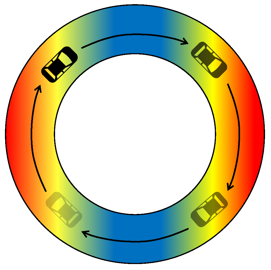
State  $(x,t)$ is the agent’s position at time t. $(x,t)\in \mathcal{X}\times \mathcal{T}$.

2. 

Action  $u(x,t)$ is the velocity of the agent at position x at time t. The optimal velocity evolves as time progresses.

3. 

Cost  $f(u,\rho )$ is the congestion cost depending on agents’ action u and population density ρ.

4. 

Value function  $V(x,t)$ is the minimum cost of the generic agent starting from position x at time t. $V_t,V_x$ are partial derivatives of $V(x,t)$ with respect to $t,x$, respectively. ${\mathit{V}}_T$ denotes the terminal cost.

Definition 2 (Mean Field Equilibrium (MFE)).

In an ST-MFG, $(u^{*}(x,t),{\rho }^{*}(x,t)),\forall (x,t)\in \mathcal{X}\times \mathcal{T}$ is called an MFE if the following conditions hold: (1) ${\rho }_t^{*}+{({\rho }^{*}·u^{*})}_x=0$; (2) $V_t^{*}+u^{*}{V}_x^{*}+f(u^{*},{\rho }^{*})=0$; (3) $u^{*}=argmi{n}_p\{f(p,\rho )+p{V}_x\}$.

In this work, we adopt a neural operator to find MFE.

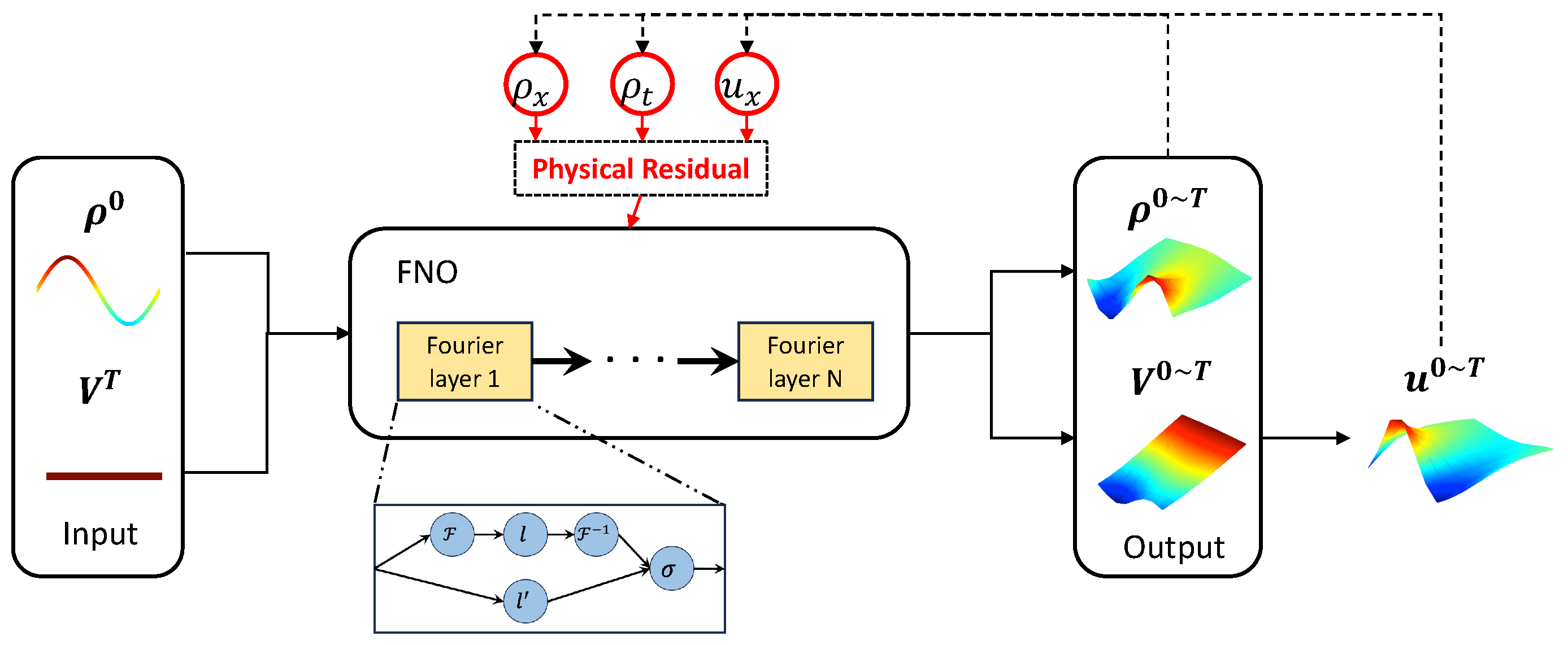
2.2. Physics-Informed Neural Operator (PINO)

The Physics-Informed Neural Operator (PINO) is an innovative approach designed to address partial differential equations (PDEs) with a focus on high computational efficiency [7]. At its core, PINO utilizes a Fourier Neural Operator (FNO) as its foundational component [5], which enables the learning of operators mapping between infinite-dimensional function spaces. This is achieved through the application of Fourier transformations, facilitating the projection of inputs into a higher-dimensional space where relationships between variables can be modeled more effectively. The PINO framework incorporates physics-informed regularization by embedding the physical laws governing the system into the loss function, ensuring that predictions adhere to known dynamics. Unlike traditional Physics-Informed Neural Networks (PINNs) that might struggle with efficiently propagating information across various conditions, PINO excels by leveraging the Fourier transformation within the FNO framework. This transformation projects boundary conditions into a higher dimensional space, thereby facilitating the seamless integration of initial or other boundary conditions into the learning process.

This unique capability of PINO to utilize Fourier transformations is particularly advantageous in handling complex problems like solving ST-MFGs that demand consideration of varying initial population densities. Traditionally, addressing such problems would require the cumbersome and computationally intensive task of retraining multiple PINNs for each new initial condition. However, PINO avoids this by offering a scalable learning framework that can adapt to different initial conditions without the need for retraining. This not only underscores the model’s computational efficiency but also highlights its flexibility and robustness in solving PDEs across a broad spectrum of conditions.

3. Learning ST-MFGs via PINOs

We introduce our PINO framework to capture population dynamics and system value functions. The dynamics of ST-MFGs are influenced by initial densities and terminal value functions, and bounded by the periodicity of x on the ring road, i.e., $\rho (0,t)=\rho (1,t)$, $u(0,t)=u(1,t)$, $\forall t\in \mathcal{T}$. Figure 1 depicts the workflow of our proposed framework, where the PINO module employs a Fourier neural operator (FNO) to represent the population density ${\mathit{\rho }}_{0-T}$ and value functions ${\mathit{V}}_{0-T}$ over time. The FNO is updated according to the physical residual that adheres to the Fokker–Planck–Kolmogorov (FPK) equation. This rule elucidates the interplay between population evolution and velocity control. The FNO also expresses the propagation of the system value function according to the Hamilton–Jacobi–Bellman (HJB) equation. Then, the optimal velocity, represented as ${\mathit{u}}_{0-T}$, is derived from the HJB, considering the given population density ${\mathit{\rho }}_{0-T}$. We further elaborate PINO framework in the following parts.

3.1. FPK Module

As shown in Figure 1, the initial density ${\mathit{\rho }}_0$ over the space domain $\mathcal{X}$ in ST-MFG serves as the FPK module input for PINO. It is linearly merged with the HJB module input and processed by the FNO. The output of the FPK module is the population density over a spatiotemporal domain ${\mathit{\rho }}_{0-T}$. FNO is composed of N Fourier layers. Each layer performs a Fourier transform $\mathcal{F}$ to capture frequency–domain features by decomposing the signals into Eigenmodes. Following a linear transformation l to eliminate the high-frequency signals, an inverse Fourier transform ${\mathcal{F}}^{-1}$ is applied to recover them. Furthermore, for each layer, a linear transformation $l^{\prime }$ is also applied to capture time–domain features. The combined output from these transformations is then passed through a nonlinear activation function $\sigma$ for the subsequent Fourier layers.

The training of the FNO for the FPK module follows the residual (marked in red) determined by the FPK equation of population evolution. Mathematically, the residual $R_{FPK}$ is calculated as

$$\begin{array}{c}\hfill R_{FPK}=\frac{{\sum }_{{\mathit{\rho }}_0\in {\mathit{\rho }}^{\mathcal{D}}}{L}_{FPK}({\mathit{\rho }}_0,{\mathcal{G}}_{\theta }({\mathit{\rho }}_0,{\mathit{V}}_T))}{|{\mathit{\rho }}^{\mathcal{D}}|},\end{array}$$

(7)

where the set ${\mathit{\rho }}^{\mathcal{D}}$ is the training set containing various initial densities. $L_{FPK}({\mathit{\rho }}_0,{\mathcal{G}}_{\theta })$ is the physics loss, which is calculated as

$$\begin{array}{c}\hfill L_{FPK}=\alpha \left|\right|{\mathcal{G}}_{\theta }{|}_{t=0}-{\mathit{\rho }}_0{\left|\right|}^2+\beta \left|\right|\frac{\partial {\mathcal{G}}_{\theta }}{\partial t}+\frac{\partial ({\mathcal{G}}_{\theta }·u)}{\partial x}{\left|\right|}^2.\end{array}$$

(8)

The first term of the physics loss function measures the gap between the operator’s output at time zero and the initial density. Meanwhile, the second term measures the physical deviation using Equation (3). Weight parameters, denoted as $\alpha$ and $\beta$, are employed to tune the relative significance of these terms. The process culminates in the derivation of the optimal control, u, which is obtained from the HJB module.

3.2. HJB Module

We solve the HJB equation (Equation (5)) to determine the optimal velocity, given the population dynamics. Since HJB is an inverse process of FPK, and the propagation rules of FPK and HJB are the same, we use the same FNO as the FPK module. Combined with the initial density ${\mathit{\rho }}_0$, the terminal costs ${\mathit{V}}_T$ of the ST-MFG system is input into the FNO to obtain the costs of spatiotemporal domain $V_{0-T}$.

The training of FNO for the HJB module follows the residual (marked in red) determined by the HJB equation. Mathematically, the residual $R_{HJB}$ is calculated as

$$\begin{array}{c}\hfill R_{HJB}=\frac{{\sum }_{{\mathit{V}}_T\in {\mathit{V}}^{\mathcal{D}}}{L}_{HJB}({\mathit{V}}_T,{\mathcal{G}}_{\theta }({\mathit{\rho }}_0,{\mathit{V}}_T))}{|{\mathit{V}}^{\mathcal{D}}|},\end{array}$$

(9)

where the set ${\mathit{V}}^{\mathcal{D}}$ is the training set containing various terminal values over the spatial domain $\mathcal{X}$. $L_{HJB}({\mathit{V}}_T,{\mathcal{G}}_{\theta })$ is the physics loss, which is calculated as

$$\begin{array}{c}\hfill L_{HJB}=\alpha \left|\right|{\mathcal{G}}_{\theta }{|}_{t=T}-{\mathit{V}}_T{\left|\right|}^2+\beta \left|\right|\frac{\partial {\mathcal{G}}_{\theta }}{\partial t}+\frac{\partial ({\mathcal{G}}_{\theta }·u)}{\partial x}{\left|\right|}^2.\end{array}$$

(10)

The first term of the physics loss function measures the discrepancy between the operator’s output in the end and the terminal values. The second term measures the physical deviation using Equation (5). Weight parameters, denoted as $\alpha$ and $\beta$, are employed to tune the relative significance of these terms. Thus, the total residual of FNO is $R=R_{FPK}+R_{HJB}$.

We calculate the optimal control $u_{0-T}$ after obtaining ${\rho }_{0-T}$ and $V_{0-T}$. Numerical methods commonly employed for solving the HJB equation include backward induction [16], the Newton method [26], and variational inequality [27]. Learning-based methods, such as RL [28,29] and PIDL [25], can also be used for solving the HJB equation. In this work, we adopt backward induction since the dynamics of the agents and the cost functions are known in the MFG system.

4. Solution Approach

We develop Algorithm 1 based on the proposed scalable learning framework in the autonomous driving velocity control scenario. A population of autonomous vehicles (AVs) navigate a ring road (Figure 2). At the time t, a generic AV selects $u(x,t)$ at position x. At a given moment t, a typical autonomous vehicle (AV) selects a velocity $u(x,t)$ at a specific location x on the ring road. This decision regarding speed selection influences the dynamic evolution of the population density of AVs circulating on the ring road. In this model, all AVs are considered to be homogeneous, implying that any decision made by one AV could be representative of decisions made by others in the same conditions. The primary objective of this study is to devise an optimal speed control strategy that minimizes the overall costs incurred during the specified time interval $[0,T]$ for a representative AV. Through the application of mathematical models and optimization techniques, it seeks to determine the most cost-effective speed profiles that can lead to an optimal distribution of AVs on the road, reducing congestion and improving the collective utility of the transportation system.

In Algorithm 1, we first initialize the neural operator ${\mathcal{G}}_{\theta }$, parameterized by $\theta$. During the ith iteration of the training process, we first sample a batch of initial population densities ${\mathit{\rho }}_0$ and terminal costs ${\mathit{V}}_T$. We use FNO to generate the population density and value function over the entire spatiotemporal domain ${\mathit{\rho }}_{0-T}$ and ${\mathit{V}}_{0-T}$. According to ${\mathit{\rho }}_{0-T}$ and ${\mathit{V}}_{0-T}$, we calculate the optimal speed ${\mathit{u}}_{0-T}^{\left(i\right)}$. The parameter ${\theta }^{\left(i\right)}$ of the neural operator is updated according to the residual. We check the following convergence conditions for ${\mathit{\rho }}_{0-T}$ and ${\mathit{V}}_{0-T}$ obtained by ${\mathcal{G}}_{\theta }({\mathit{\rho }}_0,{\mathit{V}}_T)$.

$$\begin{array}{c}\hfill \frac{{\sum }_{{\mathit{\rho }}_0\in {\mathit{\rho }}^{\mathcal{D}}}{\sum }_{{\mathit{V}}_T\in {\mathit{V}}^{\mathcal{D}}}|{\mathcal{G}}_{{\theta }^{\left(i\right)}}({\mathit{\rho }}_0,{\mathit{V}}_T)-{\mathcal{G}}_{{\theta }^{(i-1)}}({\mathit{\rho }}_0,{\mathit{V}}_T)|}{|{\mathit{\rho }}^{\mathcal{D}}\left|\right|{\mathit{V}}^{\mathcal{D}}|}<ϵ\end{array}$$

(11)

The training process moves on to the next iteration until the convergence condition holds.

Algorithm 1 PINO for ST-MFG

1: Initialization: FNO: ${\mathcal{G}}_{{\theta }^{\left(0\right)}}$;   2: for $i\leftarrow 0$ to I do   3:     Sample a batch of initial densities ${\mathit{\rho }}_0$ and terminal values ${\mathit{V}}_T$ from the training set;   4:     Generate ${\mathit{\rho }}_{0-T}^{\left(i\right)}$ and ${\mathit{V}}_{0-T}^{\left(i\right)}$ using the neural operator ${\mathcal{G}}_{{\theta }^{\left(i\right)}}({\mathit{\rho }}_0,{\mathit{V}}_T)$;   5:     for each ${\mathit{\rho }}_{0-T}^{\left(i\right)}$ and ${\mathit{V}}_{0-T}^{\left(i\right)}$ generated by FNO do   6:         for $t\leftarrow T$ to 1 do   7:            $u_{t-1}^{\left(i\right)}\leftarrow argmi{n}_u\{f(u,\rho )+u{V}_x(t,x)\}$;   8:         end for   9:         Obtain ${\mathit{u}}_{0-T}^{\left(i\right)}$ and calculate ${\mathit{u}}_x^{\left(i\right)}$; 10:     end for 11:     Obtain residual $R_{{\theta }^{\left(i\right)}}$ according to Equations (7) and (9); 12:     Update the neural operator to obtain ${\mathcal{G}}_{{\theta }^{(i+1)}}$ according to Equations (8) and (10); 13:     Check convergence (Equation (11)). 14: end for 15: Output ${\mathit{\rho }}_{0-T}$, ${\mathit{V}}_{0-T}$, ${\mathit{u}}_{0-T}$

We evaluate two PINN-based algorithms for solving ST-MFGs, as detailed in [25]. The first, a hybrid RL and PIDL approach, employs an iterative process where the HJB equation is solved via the advantage actor-critic method, and the FPK equation is addressed using a PINN. This approach allows for the dynamic updating of agents’ actions and the population’s distribution in response to evolving game conditions, leveraging the strengths of both RL and PIDL. The second is a pure PIDL algorithm that updates agents’ states and population density altogether using two PINNs. We refer to these baseline algorithms as “RL-PIDL” and “Pure-PIDL”, respectively.

Both algorithms, RL-PIDL and Pure-PIDL, offer significant advantages over conventional methods [26,27] in the context of autonomous driving MFGs. Notably, they are not restricted by the spatiotemporal mesh granularity, enhancing their ability to learn the MFE efficiently. Pure-PIDL, in particular, demonstrates superior efficiency in scenarios where the dynamics of the environment are known, requiring less training time and space compared to RL-PIDL. However, despite their advancements over traditional numerical methods, both RL-PIDL and Pure-PIDL encounter challenges concerning the propagation of information from initial conditions. This limitation necessitates the assignment and retraining of new NNs for various initial population densities, a process that significantly hampers the efficiency and scalability [7]. Conversely, our PINO framework effectively addresses these limitations, avoiding the memory and efficiency constraints observed in the baseline models.

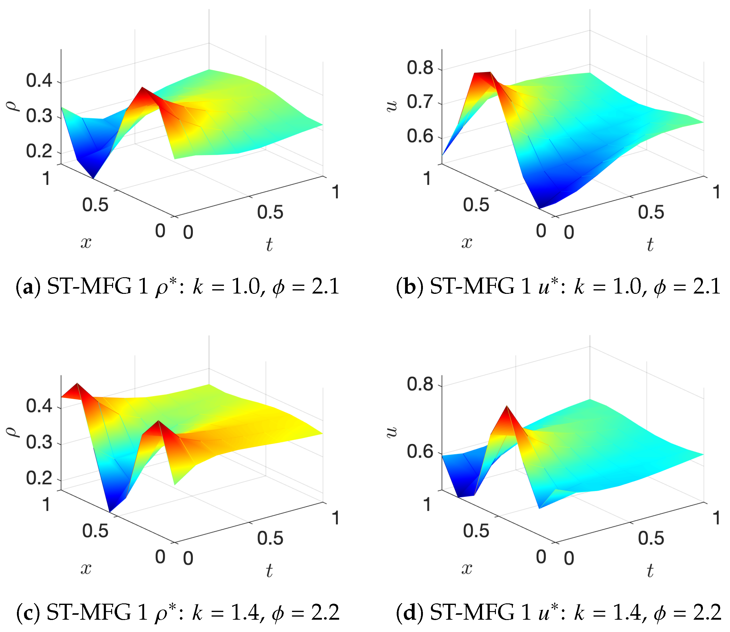
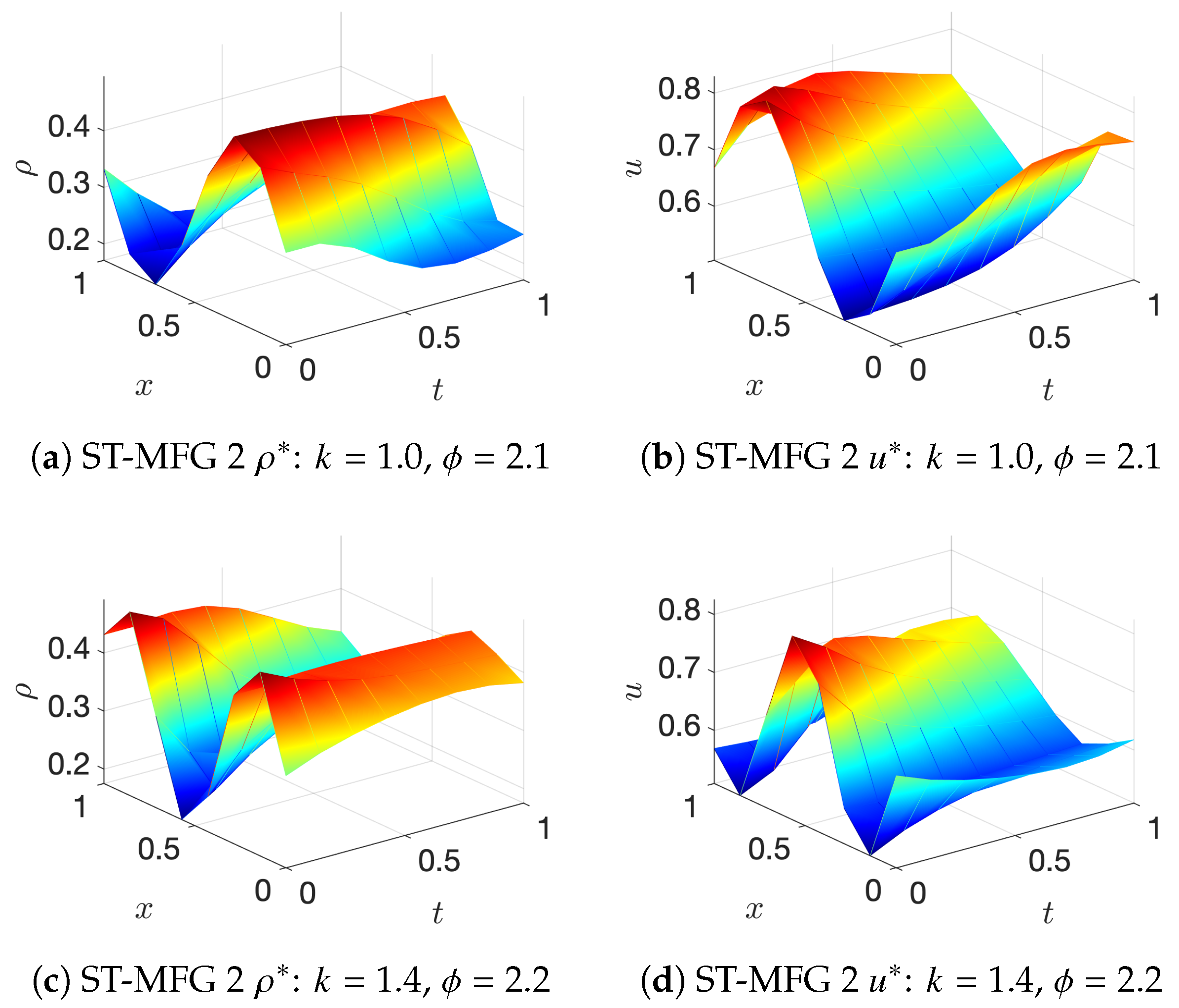
5. Numerical Experiments

We conduct numerical experiments in the scenario shown in Figure 2, which are designed to explore the dynamics of a MFG focused on AV navigating a circular road network, a scenario framed by specific initial and terminal conditions. The initial condition for this MFG is the distribution of AV population $\rho (x,0)$ over the ring road when $t=0$ and the preference $V(x,T)$ for their location when $t=T$. To model the initial distribution $\rho (x,0)$ of AVs, we utilize sinusoidal wave functions characterized by the formula $(\varphi +sin(2\pi kx\left)\right)/6$, where k represents the ordinary frequency and $\varphi$ denotes the phase of the wave. Both k and $\varphi$ are randomly selected from uniform distributions, specifically $\mathcal{U}(0.1,2.1)$ for k and $\mathcal{U}(1.5,2)$ for $\varphi$. This approach ensures a wide range of sinusoidal patterns, reflecting diverse initial traffic distributions, as illustrated in Figure 3, which shows a selection of initial density curves drawn from our training set ${\mathit{\rho }}^{\mathcal{D}}$. We assume AVs have no preference for their locations at time T, i.e., $V(x,T)=0,\forall x\in [0,1]$. The boundary condition for this MFG is the periodicity of x.

Figure 4 demonstrates the performance of the algorithm in solving ST-MFGs. The x-axis represents the iteration index during training. Figure 4a displays the convergence gap, calculated as $|{\rho }^{\left(i\right)}-{\rho }^{(i-1)}|$. Figure 4b displays the 1-Wasserstein distance (W1-distance), which measures the closeness [30] between our results and the MFE (mean field equilibrium) obtained by numerical methods, represented as $|{\rho }^{\left(i\right)}-{\rho }^{*}|$. Our proposed algorithm converges to the MFE after 200 iterations.

Figure 5 and Figure 6 demonstrate the population density ${\rho }^{*}$ and velocity choice $u^{*}$ at MFE for an unseen initial density in two different ST-MFG settings. We implement our methods on the ST-MFG with 2 cost functions:

• ST-MFG1: The cost function is

  $$\begin{array}{c}\hfill f(u,\rho )=\underset{\mathrm{energy}}{\underbrace{\frac{1}{2}{\left(\frac{u}{u_{max}}\right)}^2}}-\underset{\mathrm{efficiency}}{\underbrace{\frac{u}{u_{max}}}}+\underset{\mathrm{safety}}{\underbrace{\frac{u\rho }{u_{max}{\rho }_{jam}}}}.\end{array}$$

  (12)

In this model, AVs tend to decelerate in high-density areas and accelerate in low-density areas.

2.

ST-MFG2: The Lighthill–Whitham–Richards model is a traditional traffic flow model where the driving objective is to maintain some desired speed. The cost function is

$$\begin{array}{c}\hfill f(u,\rho )=\frac{1}{2}{(U\left(\rho \right)-u)}^2\end{array}$$

(13)

where, $U\left(\rho \right)$ is an arbitrary desired speed function with respect to density $\rho$. It is straightforward to find that the analytical solution of the LWR model is $u=U\left(\rho \right)$, which means that at MFE, vehicles maintain the desired speed on roads.

Figure 5. Population density ${\rho }^{*}$ and speed choice $u^{*}$ at MFE for ST-MFG 1.

Figure 5. Population density ${\rho }^{*}$ and speed choice $u^{*}$ at MFE for ST-MFG 1.

Figure 6. Population density ${\rho }^{*}$ and speed choice $u^{*}$ at MFE for ST-MFG 2.

Figure 6. Population density ${\rho }^{*}$ and speed choice $u^{*}$ at MFE for ST-MFG 2.

The population of AVs incurs a penalty in ST-MFG 1 if they select the same velocity control. The x-axis represents position x, and the y-axis represents time t. Figure 5a,b and Figure 6a,b have an initial density with $k=1.0,\varphi =2.1$. Figure 5c,d and Figure 6c,d have an initial density with $k=1.4,\varphi =2.2$. Compared to the equilibrium ${\rho }^{*}$ in ST-MFG 2, the population density and velocity in ST-MFG 1 dissipate without waveforms, demonstrating smoother traffic conditions at time T.

Table 1. Comparison of existing learning methods.

		PINO	RL-PIDL	Pure-PIDL
Memory (Number of NNs)		1	48	32
Time (s)	ST-MFG 1	$46.56$	$1488.53$	$742.25$
	ST-MFG 2	$44.68$	$1210.14$	$421.64$

compares the total training time (unit: s) required for solving ST-MFGs with various initial conditions with different learning methods.

We summarize the results from our numerical experiments as follows:

(1) Our proposed PINO needs fewer neural networks (NNs) and shorter training time compared to PINN-based algorithms, demonstrating the scalability of our method. This is because the input of neural architecture in the PINN framework fails to capture various boundary conditions, which leads to an iterative training process to solve MFEs. In a comparison to PINN, PINO is scalable to initial population density along with terminal cost among the space domain.

(2) In this study, the PINO-based learning method is designed to significantly enhance the adaptability of neural networks across various initial conditions. This advancement is pivotal for tackling large-scale Mean Field Games (MFGs), especially within graph-based frameworks. The applications of this method are broad and diverse, encompassing, but not limited to, managing autonomous vehicles on road networks, analyzing pedestrian or crowd movements, optimizing vehicle fleet network operations, routing internet packets efficiently, understanding social opinion trends, and tracking epidemiological patterns.

6. Conclusions

This work presents a scalable learning framework for solving coupled forward–backward PDE systems using a physics-informed neural operator (PINO). PINO allows for efficient training of the forward PDE with varying initial conditions. Compared to traditional physics-informed neural networks (PINNs), our proposed framework overcomes memory and efficiency limitations. We also demonstrate the efficiency of this method on a numerical example motivated by optimal autonomous driving control. The PINO-based framework offers a memory- and data-efficient approach for solving complex PDE systems with generalizability similar to PDE systems, differing only in boundary conditions.

This work is motivated by the computational challenge faced by the mean field game (MFG). MFGs have gained increasing popularity in recent years in finance, economics, and engineering due to its power to model the strategic interactions among a large number of agents in multi-agent systems. The equilibria associated with MFGs, also known as mean field equilibra (MFE), are challenging to solve due to their coupled forward and backward PDE structure. That is why computational methods based on machine learning have gained momentum. The PINO-based learning method developed in this study empowers the generalization of the trained neural networks to various initial conditions, which holds the potential to solve large-scale MFGs, in particular, graph-based applications, including but not limited to optimization of autonomous vehicle navigation in complex road networks, the management of pedestrian or crowd movements in urban environments, the efficient coordination of vehicle fleet networks, the strategic routing of Internet packets to enhance network efficiency, the analysis of social opinion dynamics to understand societal trends, and the study of epidemiological models to predict the spread of diseases.

References

- Raissi, M.; Perdikaris, P.; Karniadakis, G.E. Physics-informed neural networks: A deep learning framework for solving forward and inverse problems involving nonlinear partial differential equations. J. Comput. Phys. 2019, 378, 686–707. [Google Scholar] [CrossRef]
- Mo, Z.; Fu, Y.; Di, X. PI-NeuGODE: Physics-Informed Graph Neural Ordinary Differential Equations for Spatiotemporal Trajectory Prediction. In Proceedings of the 23rd International Conference on Autonomous Agents and Multiagent Systems, AAMAS, London, UK, 29 May–2 June 2023. [Google Scholar]
- Di, X.; Shi, R.; Mo, Z.; Fu, Y. Physics-Informed Deep Learning for Traffic State Estimation: A Survey and the Outlook. Algorithms 2023, 16, 305. [Google Scholar] [CrossRef]
- Shi, R.; Mo, Z.; Di, X. Physics-informed deep learning for traffic state estimation: A hybrid paradigm informed by second-order traffic models. In Proceedings of the AAAI Conference on Artificial Intelligence, Virtual, 2–9 February 2021; Volume 35, pp. 540–547. [Google Scholar]
- Li, Z.; Kovachki, N.; Azizzadenesheli, K.; Liu, B.; Bhattacharya, K.; Stuart, A.; Anandkumar, A. Fourier neural operator for parametric partial differential equations. arXiv 2020, arXiv:2010.08895. [Google Scholar]
- Thodi, B.T.; Ambadipudi, S.V.R.; Jabari, S.E. Learning-based solutions to nonlinear hyperbolic PDEs: Empirical insights on generalization errors. arXiv 2023, arXiv:2302.08144. [Google Scholar]
- Li, Z.; Zheng, H.; Kovachki, N.; Jin, D.; Chen, H.; Liu, B.; Azizzadenesheli, K.; Anandkumar, A. Physics-informed neural operator for learning partial differential equations. arXiv 2021, arXiv:2111.03794. [Google Scholar] [CrossRef]
- Lasry, J.M.; Lions, P.L. Mean field games. Jpn. J. Math. 2007, 2, 229–260. [Google Scholar] [CrossRef]
- Huang, M.; Malhamé, R.P.; Caines, P.E. Large population stochastic dynamic games: Closed-loop McKean-Vlasov systems and the Nash certainty equivalence principle. Commun. Inf. Syst. 2006, 6, 221–252. [Google Scholar]
- Cardaliaguet, P. Notes on Mean Field Games; Technical Report; Stanford University: Stanford, CA, USA, 2010. [Google Scholar]
- Cardaliaguet, P. Weak solutions for first order mean field games with local coupling. In Analysis and Geometry in Control Theory and Its Applications; Springer: Cham, Switzerland, 2015; pp. 111–158. [Google Scholar]
- Kizilkale, A.C.; Caines, P.E. Mean Field Stochastic Adaptive Control. IEEE Trans. Autom. Control. 2013, 58, 905–920. [Google Scholar] [CrossRef]
- Yin, H.; Mehta, P.G.; Meyn, S.P.; Shanbhag, U.V. Learning in Mean-Field Games. IEEE Trans. Autom. Control 2014, 59, 629–644. [Google Scholar] [CrossRef]
- Yang, J.; Ye, X.; Trivedi, R.; Xu, H.; Zha, H. Deep Mean Field Games for Learning Optimal Behavior Policy of Large Populations. In Proceedings of the International Conference on Learning Representations, Vancouver, BC, Canada, 30 April–3 May 2018. [Google Scholar]
- Elie, R.; Perolat, J.; Laurière, M.; Geist, M.; Pietquin, O. On the convergence of model free learning in mean field games. In Proceedings of the AAAI Conference on Artificial Intelligence, New York, NY, USA, 7–12 February 2020; pp. 7143–7150. [Google Scholar]
- Perrin, S.; Laurière, M.; Pérolat, J.; Geist, M.; Élie, R.; Pietquin, O. Mean Field Games Flock! The Reinforcement Learning Way. In Proceedings of the International Joint Conference on Artificial Intelligence (IJCAI-21), Virtual, 19–26 August 2021. [Google Scholar]
- Mguni, D.; Jennings, J.; de Cote, E.M. Decentralised learning in systems with many, many strategic agents. In Proceedings of the Thirty-Second AAAI Conference on Artificial Intelligence, New Orleans, LA, USA, 2–7 February 2018. [Google Scholar]
- Subramanian, S.; Taylor, M.; Crowley, M.; Poupart, P. Decentralized Mean Field Games. In Proceedings of the AAAI Conference on Artificial Intelligence, Palo Alto, CA, USA, 22 February–1 March 2022. [Google Scholar]
- Chen, X.; Liu, S.; Di, X. Learning Dual Mean Field Games on Graphs. In Proceedings of the 26th European Conference on Artificial Intelligence, ECAI, Krakow, Poland, 30 September–4 October 2023. [Google Scholar]
- Reisinger, C.; Stockinger, W.; Zhang, Y. A fast iterative PDE-based algorithm for feedback controls of nonsmooth mean-field control problems. arXiv 2022, arXiv:2108.06740. [Google Scholar]
- Cao, H.; Guo, X.; Laurière, M. Connecting GANs, MFGs, and OT. arXiv 2021, arXiv:2002.04112. [Google Scholar]
- Ruthotto, L.; Osher, S.J.; Li, W.; Nurbekyan, L.; Fung, S.W. A machine learning framework for solving high-dimensional mean field game and mean field control problems. Proc. Natl. Acad. Sci. USA 2020, 117, 9183–9193. [Google Scholar] [CrossRef] [PubMed]
- Carmona, R.; Laurière, M. Convergence Analysis of Machine Learning Algorithms for the Numerical Solution of Mean Field Control and Games I: The Ergodic Case. SIAM J. Numer. Anal. 2021, 59, 1455–1485. [Google Scholar] [CrossRef]
- Germain, M.; Mikael, J.; Warin, X. Numerical resolution of McKean-Vlasov FBSDEs using neural networks. Methodol. Comput. Appl. Probab. 2022, 24, 2557–2586. [Google Scholar] [CrossRef]
- Chen, X.; Liu, S.; Di, X. A Hybrid Framework of Reinforcement Learning and Physics-Informed Deep Learning for Spatiotemporal Mean Field Games. In Proceedings of the 22nd International Conference on Autonomous Agents and Multiagent Systems, AAMAS ’23, London, UK, 29 May–2 June 2023. [Google Scholar]
- Huang, K.; Di, X.; Du, Q.; Chen, X. A game-theoretic framework for autonomous vehicles velocity control: Bridging microscopic differential games and macroscopic mean field games. Discret. Contin. Dyn. Syst. D 2020, 25, 4869–4903. [Google Scholar] [CrossRef]
- Huang, K.; Chen, X.; Di, X.; Du, Q. Dynamic driving and routing games for autonomous vehicles on networks: A mean field game approach. Transp. Res. Part C Emerg. Technol. 2021, 128, 103189. [Google Scholar] [CrossRef]
- Guo, X.; Hu, A.; Xu, R.; Zhang, J. Learning Mean-Field Games. In Proceedings of the Advances in Neural Information Processing Systems; Curran Associates, Inc.: Red Hook, NY, USA, 2019; Volume 32. [Google Scholar]
- Perrin, S.; Perolat, J.; Laurière, M.; Geist, M.; Elie, R.; Pietquin, O. Fictitious Play for Mean Field Games: Continuous Time Analysis and Applications. In Proceedings of the 34th International Conference on Neural Information Processing Systems, NIPS’20, Virtual, 6–12 December 2020. [Google Scholar]
- Lauriere, M.; Perrin, S.; Girgin, S.; Muller, P.; Jain, A.; Cabannes, T.; Piliouras, G.; Perolat, J.; Elie, R.; Pietquin, O.; et al. Scalable Deep Reinforcement Learning Algorithms for Mean Field Games. In Proceedings of the 39th International Conference on Machine Learning, Baltimore, MD, USA, 17–23 July 2022; Volume 162, pp. 12078–12095. [Google Scholar]