Inferencing Space Travel Pricing from Mathematics of General Relativity Theory, Accounting Equation, and Economic Functions

Abstract

This study derives space travel pricing by Walrasian Equilibrium, which is logical reasoning from the general relativity theory (GRT), the accounting equation, and economic supply and demand functions. The Cobb–Douglas functions embed the endogenous space factor as new capital to form the space travel firm’s production function, which is also transformed into the consumer’s utility function. Thus, the market equilibrium occurs at the equivalence of supply and demand functions, like the GRT, which presents the equivalence between the spatial geometric tensor and the energy–momentum tensor, explaining the principles of gravity and the motion of space matter in the spacetime framework. The mathematical axiomatic set theory of the accounting equation explains the equity premium effect that causes a short-term accounting equation inequality, then reaches the equivalence by suppliers’ incremental equity through the closing accounts process of the accounting cycle. On the demand side, the consumption of space travel can be assumed as a value at risk (VaR) investment to attain the specific spacetime curvature in an expected orbit. Spacetime market equilibrium is then achieved to construct the space travel pricing model. The methodology of econophysics and the analogy method was applied to infer space travel pricing with the model of profit maximization, single-mindedness, and envy-free pricing in unit-demand markets. A case study with simulation was conducted for empirical verification of the mathematical models and algorithm. The results showed that space travel pricing remains associated with the principle of market equilibrium, but needs to be extended to the spacetime tensor of GRT.

1. Introduction

Space tourism began with Dennis Tito’s private trip to the International Space Station, costing USD 20 million, in 2001 [1]. With the emergence of private space companies such as SpaceX, Blue Origin, and Virgin Galactic, there has been growing interest in a market to make space travel more accessible to private individuals [1,2]. Space tourism has many attributes that differ from Earth tourism, like untraditional suppliers, selected tourists, and asymmetric market equilibria [3]. One of the unique attributes of space travel is its ultra-expensive prices. For example, the Virgin Galactic reservation quantity increased from less than 100 in 2006 to over 1000 in 2023, and the bidding price increased from USD 250,000 to 450,000 [4]. The first research question is, why is space travel so expensive? This study aims to infer the space travel pricing mechanism by the analogy of general relativity theory (GRT) in the physical field and the accounting equation in the economic field.

GRT, developed by Albert Einstein, discusses gravitation and has been tested as a solid scientific fundamental to physics and cosmology [5]. The theory describes gravity as the spacetime curvature bent by mass and energy. In GRT, mass and energy warp the fabric of space and time, affecting the motion of matter and the passage of spacetime itself [6]. It is worth discussing space travel behavior concerns about GRT, because human travel has been flown above the Earth’s surface into space, reaching the height from zero to the nonzero curvature of spacetime [7]. Space travel pricing cannot be derived from airplane pricing models, because the former attains nonzero spacetime curvature behind the Kármán line and the latter fly flat at a spacetime curvature below a 20 km height [8]. The second research question is how to derivate the space travel pricing model. The accounting equation with axiomatic set theory, the production and utility functions embedded space factor, and pricing problems in computer science are adopted to infer space travel pricing.

The accounting equation, with assets equal to the sum of liabilities and equity, forms the basis of accounting principles [9]. Juárez [10] used a mathematical axiomatic set theory indicating the inequality of the accounting equation. The analysis determined that the sets of assets do not equal liabilities plus equity without financial meaning. However, this study inferred that inequality happens in a dynamic adjustment period when the expected space travel profit causes equity premium effects; thus, the inequality of the accounting equation only happens in a short period. In accounting, the net income will be brought forward to become incremental equity to balance the accounting equation after the closing account stage in the accounting cycle. The space travel pricing model can then be derived during the adjustment period of the supplier’s accounting equation. Moreover, this study explains the pricing model from the economic supply side and demand and market equilibrium perspectives. The production and consumer functions of market equilibrium are discussed when integrating the principles of GRT and the accounting equation in solving space travel pricing questions.

2. Mathematics of General Relativity Applied in Space Travel

2.1. The Mathematics of General Relativity Applied on Space Travel

GRT explains that the gravitational effect between masses results from their warping of spacetime. GRT presents that matter tells spacetime how to curve, and curved spacetime tells matter how to move [11], as indicated in Figure 1. The implication of GRT for space travel is that flying to a nonzero curvature needs the equivalent of energy–momentum according to the transformation of energy efficiency based on a firm’s space technological assets, defined as a new capital factor in the production function [12]. This function is discussed later.

Its mathematics involve differential geometry and tensor calculus, where concepts like manifolds, tangent spaces, covariant differentiation, and curvature are rigorously defined [13]. At the core of GRT are the Einstein Field Equations, which describe how Einstein tensor equals energy–momentum tensor [14], as indicated in Equation (1).

$$R_{\mu v}-\frac{1}{2}R{g}_{\mu v}=\frac{8\pi G}{c^4}{T}_{\mu v},$$

(1)

where $R_{\mu v}$ is the Ricci curvature tensor; R is the Ricci scalar; $g_{\mu v}$ is the metric tensor; $T_{\mu \nu }$ is the energy–momentum tensor; G is the Newtonian constant of gravitation; c is the speed of light; and $\mu ,v$ are the spacetime coordinates.

Equation (1) and Figure 1 can be realized as the space vehicle flying to the designated orbit with a specific spacetime curvature, which needs to reach the required cosmic velocity depending on the energy efficiency [15]. The space technology involved includes mixed fuel, engine technology, reusable launch vehicles, electromechanical and communication systems, and ground control systems, as well as intelligent manned space vehicles [16]. Therefore, Equation (1) represents the energy distribution equation required for traveling to the geometrical space orbit. In other words, a supplier must offer the equivalent energy–momentum at the same level as the orbital energy distribution [17].

2.2. Accounting Equation Implies Capital Investment and Assets

The accounting equation indicates that a company’s assets are equal to the sum of liabilities and the owner’s equity [18], as shown in Equation (2). The equation demonstrates that all the assets used for business operations are from the funding sources of liabilities and equity. This study applies the equation to argue that the capital assets of a space firm come from the funding sources of its investments. It can be metaphoric to the GRT’s Einstein and energy–momentum tensors in Equation (1). The accounting equation has been recognized as the standard system businesses use to record financial transactions, including space travel deals.

Assets = Liabilities + Owner’s Equity

(2)

Equation (2) means that the value of assets (A) is equal to and comes from the funding value of liabilities (L) and the owner’s equity (E) [19]. However, Juárez [10] argued the accounting equation’s inequality by applying axiomatic set theory and predicate logic. Using the axiom of union, set C comprises the elements claimed on the liabilities subset L and the equity subset E of the capital subsets. By the axiom of extensionality, the sets A and C are compared. The axiom of specification allows for determining that the capital units of each subset of C have similar capital units delivered to the subsets of A. Accordingly, the subset of A is not congruent with the subsets of C and, due to this lack of correspondence, A ≠ C and A ≠ L ∪ E. The analysis determined that the sets of assets are not equal to the sets of liabilities and equity, concluding that assets are not equal to liabilities plus equity. This inequality is interpreted within the restrictions of applying the set theory to financial data and the algebraic sum without financial meanings [20].

Nevertheless, we found that the studies of Juárez [10] and [20] might have committed Russell’s paradox, which a predicativist explanation can solve, the Cantorian solutions, or particular zig-zag solutions [21]. Ludwig Wittgenstein’s Tractatus Logico-Philosophicus claimed that no proposition can contain itself; similarly, a set cannot contain itself [22]. The sets A and C cannot contain themselves, which means they can contain each other. A given connection set can also solve Russell’s paradox of the inequity of the accounting equation. The spacetime set S can connect the conditions of the accounting equation from inequality to equality, as shown in Equation (3).

∀A ∀C (A = C ⇔ ∀S (S ∈ A ⇔ S ∈ C)).

(3)

Thus, we can infer that A = C, C = L ∪ E, and A = L ∪ E, in general, and A = L ∪ E, but the Zermelo–Fraenkel set theory is necessary [23]. Juárez’s [10] accounting equation inequality was originally deduced only by the mathematical set theory without financial meanings [10,20]. However, the physical element of spacetime set S can be implicated to connect the accounting equation, which can be interpreted with financial meanings. The set S implies that the space capital becomes a new production factor for a firm to offer a space travel product if, and only if, the accounting equation sustains, as indicated in Equation (3). The short-term dynamic accounting equation inequality issue of Equation (2) can be explained by a short-term dynamic adjustment process of the equity premium generated by capital investment when incorporating the space capital of a space travel firm during the accounting period [24]. When the accounting cycle is complete, the equality in Equation (3) is sustained with the spacetime element of the space capital at the end of an accounting period.

2.3. Equilibrium Pricing Based on Production and Consumption Functions of Space Travel

In the space industry, it is proper to apply the economic neo-classical one-sector growth model that outlines how a steady economic growth rate results from three driving forces—labor, capital, and space technology. The space capital assets developed from capital investment are defined as a spacetime production factor in the production function [25]. Potential outputs can be produced by the production factors Labor, L, and space capital, K(S), on the spacetime curvature surface. Equilibrium output is achieved when the capital investment meets labor savings. In other words, a space firm’s capital investment in advancing space technology can produce space travel products for tourists flying in orbit at different space curvatures [26]. The accounting equation elements present the capital assets and investment to produce the potential output of space travel products. The Cobb–Douglas production function can express the labor factor L and the space capital K(S) with the technological progress factor, g, as indicated in Equation (4) [27]. The equilibrium output is committed when the investment capital equals savings, as shown in Figure 2.

$${Q_s}_{ }=A{e}^g{L}^{\alpha }{K\left(S\right)}^{\beta }$$

(4)

where Q_s = total production, A = total factor productivity, $\alpha$ and $\beta$ = output elasticities of capital and labor, and g is the constant rate of technical progress.

The Cobb–Douglas functional form is used in the production theory and has become standard in microeconomic consumer theory applied as a utility function, where Q_s becomes U for utility [28]. The K(S) is then replaced with consumption items. When the utility function is maximized, subject to a budget constraint B, the individual will optimally distribute their budget among their consumption item, C(S), where C is consumption and S is the space product. In other words, the consumer will choose their preferred product C(S) of space travel at a price p under budget constraint B. The utility-maximizing problem is then presented as Equation (5).

$$\begin{array}{c}\underset{C,\mathit{S}\ge 0}{\max }U\left(C\right(S\left)\right);\mathrm{s}.\mathrm{t}.B\\ Q_d=f(p,C(S\left)\right)\end{array}$$

(5)

The intersection of Qs, Equation (4), and Qd, Equation (5), can determine the equilibrium pricing.

2.4. Space Travel Pricing Process

Based on Equations (1)–(5) and given ceteris paribus, except for valuables related to the accounting equation [29,30], a space firm’s funding sources of liabilities and owner’s equity are distributed to its space capital assets [31]. This can be analogized to the equality of the energy–momentum tensor and Einstein’s tensor. A space firm uses space capital to reach the geometric coordinate: a specific spacetime curvature of Einstein’s tensor [32] that generates equity premium, influencing its stock pricing P_s and then space travel pricing P_p. The loop will continue until competition offsets the investment effect, as shown in Figure 3. The operating revenue from space travel will be the incremental investment influencing the equity premium and space travel pricing level [33]. The causality of the space travel pricing and the supplier’s market value is then presented in Figure 3 [34,35].

3. Methodology

3.1. Econophysics Analogy

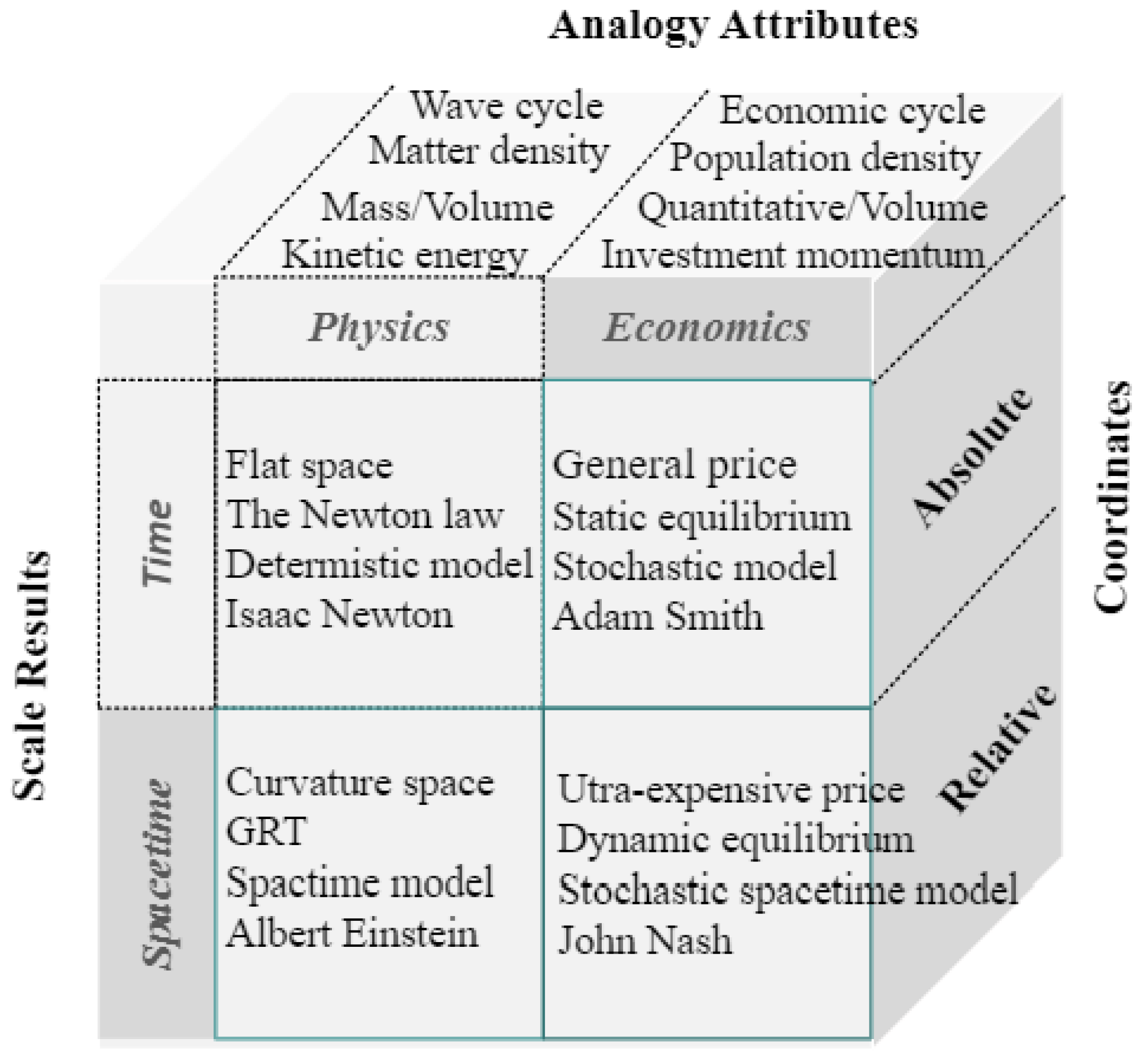
This study is interdisciplinary research covering the fields of physics and economics to infer the space travel pricing model based on GRT, the accounting equation, and economic functions. The methodology applies econophysics, which was introduced by an analogy with similar terms that describe applications of physics to different fields [36]. From the beginning, econophysics has been the application of the principles of physics to the study of financial markets under the hypothesis that the economic world behaves like a collection of electrons or a group of water molecules that interact [37]. It has always been considered as such by econophysicists, with new tools of statistical physics and recent breakthroughs in understanding chaotic systems [38]. Econophysics has alternative names, such as financial physics, arising initially from its new development of two different disciplines: finance and physics [39]. We have noticed that space pricing is prohibitive compared to ground transportation pricing. Inferring the unique space pricing behavior can be analogized with the general physical spacetime attributes in GRT, as shown in Equation (1). To bridge the gap between physics and economics, this study adopts the analogy method of the econophysics methodology, as indicated in Figure 4, to link the attributes of the two fields for the following inference of space travel pricing [1]. Figure 4 indicates that the analogy attributes of physics and economics are paired with similar meanings. It helps to infer the pricing model, no matter whether the scale is the absolute time frame or the relative spacetime tensor.

This methodology has been applied to help finance research with many innovative theories. One of the pricing models is the Black, Scholes, and Merton (BSM) pricing model, which is used to evaluate stock options by applying the thermodynamic equation to finance [40]. The BSM option pricing model involves a principle-theory-type approach as the paradigm of econophysics methodology [41]. Various principles in the pricing model possess the status of the postulates of empirical generality concerning the behavior of economic agents. Crucially, econophysicists, also using the statistical physics analogy, adopt more of a constructive-theory-type approach [41].

3.2. Proposition Development

This study follows the methodology of econophysics, applying GRT, the accounting equation, and economic functions to infer space travel pricing within the spacetime context. Thus, the assumption of a continuous spacetime manifold is needed in the pricing model [1]. In addition to GRT, the capital in the accounting equation, the production factor K(S) in the production function, and the consumption item C(S) in the utility function should all fit the assumption. The spacetime assumption is different from the assumption of the traditional pricing theory, which is that time and space are independent. The Earth flight pricing model generally takes spatial distance as a primary factor, with various pricing strategies for business classes and services [42]. Time is an independent variable in considering price setting. The farther the flying distance, the higher the ticket price can be observed in the flight market. Time is only an independent factor that corresponds to the space distance. Temporal span does not necessarily have an equal proportionality with the space transition [43]. For example, the price of a direct flight in a short time is high, which implies that time and space are independent variables of pricing behavior.

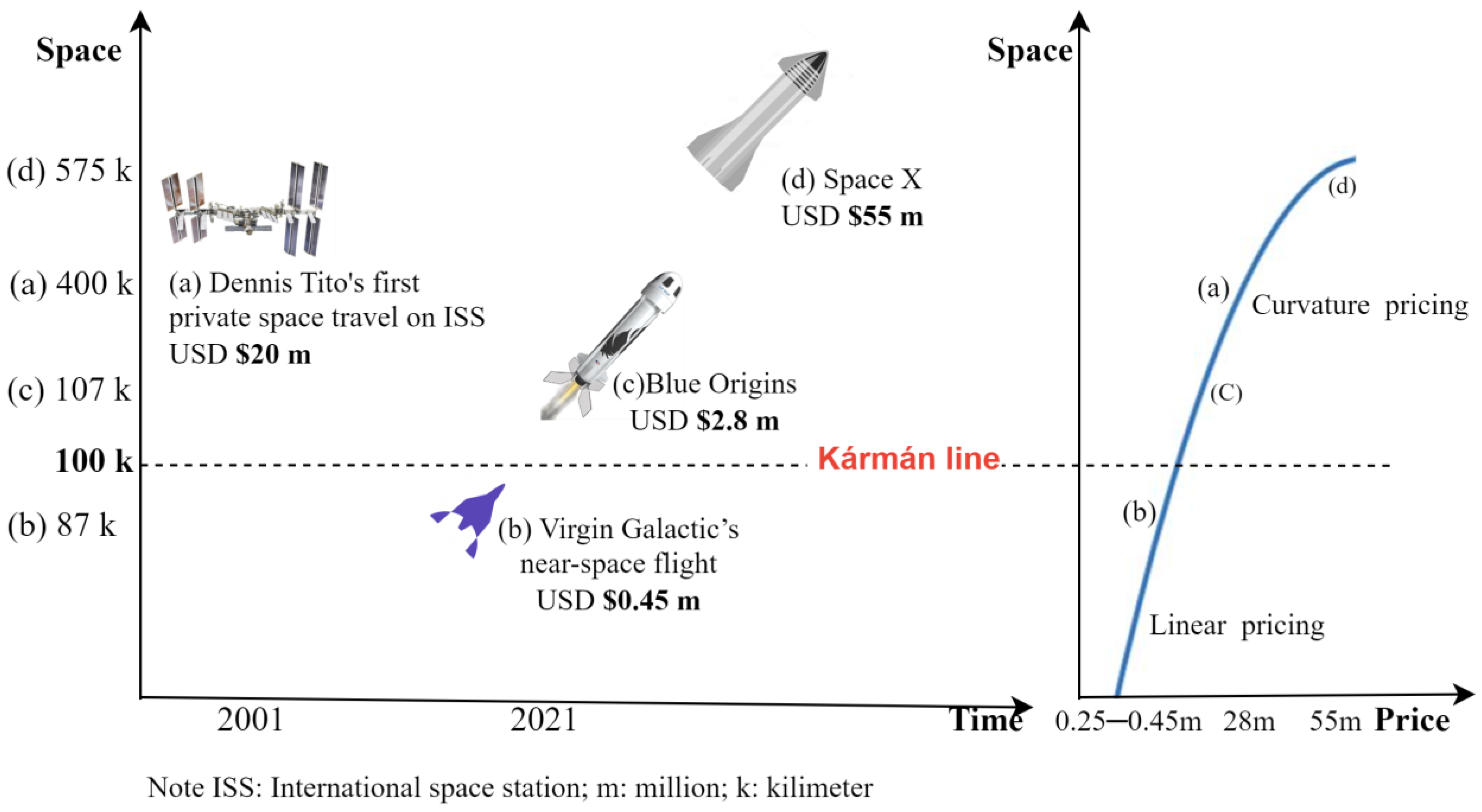
However, the space pricing model should be updated after applying the spacetime tensor construct. According to the time dilation in GRT spacetime, the pricing model must be interpreted using the Minkowski or Schwarzschild spacetime formula [44]. In space travel pricing behavior, we observe that Virgin Galactic, Blue Origins, and SpaceX have various pricing, as shown in Figure 5. Blue Origins flies about 107 km above the Earth’s surface, which is about 1.2 times higher than Virgin Galactic, which flies at a height of 87 km, but the ticket price is six times the difference. SpaceX’s orbital altitude is about 550 km, which is about five times higher than Blue Origins’s space altitude, with a 20-time difference in price. The relationship between pricing levels and spacetime coordinates is nonlinear [1], as shown in Figure 5.

This study argues that space travel pricing concerns the equity premium effect, which depends on the spaceship firm’s capability to reach the designed spacetime curvature. The higher the attitude, the higher the equity premium, like SpaceX compared with Virgin Galactic. We can observe the pricing behaviors involved with the spacetime curvatures of the spacecraft companies in Figure 5. Thus, this study summarizes Proposition 1 as follows:

Proposition 1:

Given the capital investment of a supplier’s spacetime curvature technology in the accounting equation, the profit maximization pricing of a space travel firm is positively influenced by the space capital.

This study proposes a spacetime pricing model that echoes GRT, which presents the equality relationship between Einstein’s tensor and energy–momentum tensor. A space supplier is willing and able to provide its space capital mapping with the equivalent energy–momentum tensor. The revenue for attaining the required spacetime curvature can be referred to the space travel pricing behavior, including production factors, cost, and elasticity. A space traveler is willing and able to pay to fly to a specific orbital spacetime curvature. The expenditure for achieving the altitude can be referred to the space travel demand pricing behavior, including a consumer’s motivation, utilities, and elasticity. Given the market equilibrium on dealt transactions, the spacetime pricing model reflects not only the supply side, but also the demand side.

Proposition 2:

Based on market equilibrium, the spacetime pricing derivations apply to the supply side and the demand side.

4. Results and Discussions

4.1. Pricing Model and Algorithm

Market pricing is a critical signal to guide participants in assessing a product’s value and making transaction decisions [45]. The space travel pricing problems and approximate results are for economic agents to decide on investment and consumption in the space travel market, which is critical in a nascent industry. The equilibrium pricing echoes the principle of the GRT about the laws of sciences having the same form in all admissible frames of reference [46]. In other words, the laws of economics have the same form in both supply and demand frames of reference. Thus, market equilibrium has always been the economic invariant, like other scientific fields.

Equation (1), GRT, is a field theory in physics, Equation (2), the accounting equation, is a field theory in economics, and Equations (3)–(5) open the dialogue between the two field theories by using the spacetime element to link the two sets of physics and economics in the space travel era. The deduction of the space travel pricing model based on mathematical logic presents a positive correlation between space travel pricing and GRT. The research result approximates the pricing problems in computer science on the themes of profit maximization, single-mindedness, and envy-free pricing in unit-demand markets [47,48,49]. Profit maximization with single-minded pricing is carried out by a space travel supplier, as determined by its capital investment, based on the accounting Equation (2) that echoes Proposition 1. Envy-free pricing can be interpreted in a unit-demand auction of space travel, where each bidder receives a ticket that maximizes their utility and the auction can maximize the supplier’s profit, which echoes Proposition 2. The pricing problems are initially non-deterministic polynomial-time hard (NP-hard). However, many algorithms and models have been developed to obtain proper approximations. For example, Fernandes et al. [50] derivated four mixed integer linear programming formulations for the pricing problem and experimentally compared them to the previous literature that concluded three models with economic interpretations. Corresponding to the pricing inference results of this study, we can consider the variant of the space travel prices to be restricted to being chosen from a geometric series, which corresponds to the spacetime curvatures of the space orbits to meet the pricing requirements of supply and demand [51].

An approximation algorithm builds on the profit maximization, single-mindedness, and envy-free pricing work in the economics literature concerning Walrasian Equilibria (WE) [52]. Given a value matrix V, a Walrasian Equilibrium (p, M) consists of envy-free pricing p and a matching M, such that all unmatched items have a price of zero. The following theorem characterizes Walrasian Equilibria in the unit-demand pricing problem [47].

Theorem 1.

Let (p, M) be a Walrasian Equilibrium. Then, M is a maximum weight matching on the value matrix V; furthermore, for any maximum matching, M0 (p, M₀) is also a Walrasian equilibrium [47].

For a value matrix V, we let $\omega$(V) denote the weight of a maximum weight matching MM(V). For an item j, let V_−j denote the value matrix with item j removed, i.e., the matrix obtained by deleting column j from V. The following Algorithm 1 finds the Walrasian Equilibrium with the highest prices to meet the maximum profit and utility for a space travel [47].

Algorithm 1. MaxWEP: Maximum Walrasian Prices.

Input: Value matrix V.

For each item j, let $\widehat{p}$j = $\omega$(V) − $\omega$(V − j).

Output: $\widehat{p}$ and MM(V).

Based on Proposition 2, V can be the maximum output on the supply side or the maximum utility on the demand side, as shown in Figure 2.

4.2. Case Study and Simulation

This study adopts a case study to analyze space travel pricing empirically. Virgin Galactic is applied to the case study because it is the only listed firm that reveals its stock and ticket prices with public financial information. Virgin Galactic was officially founded by Richard Branson on 27 September 2004 [53,54], and started its monthly commercial flights in July 2023 [55]. Its ticket pricing varies between USD 25,000 and 45,000 according to a bidding pricing mechanism, and flies to the height around an altitude of about 80 km before falling back to Earth [56].

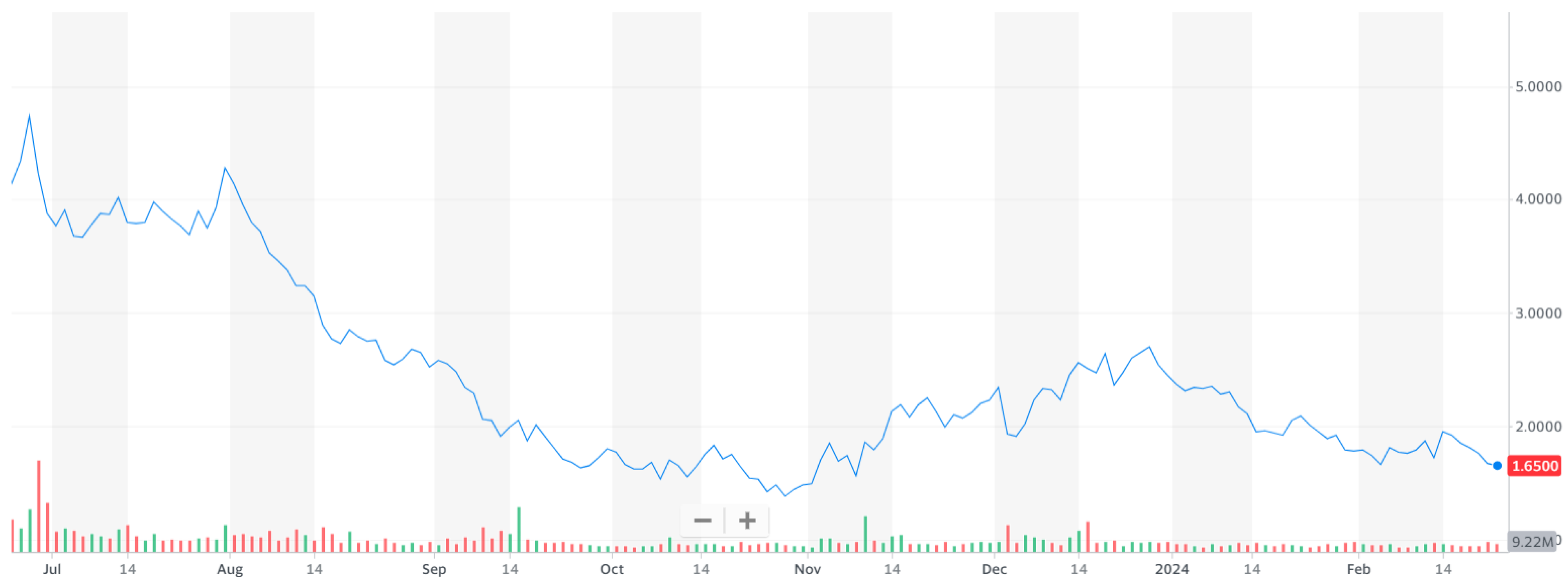
Its stock price fluctuation since the routine flight was introduced is shown in Figure 6, which has responded to its spacetime attributes, like ticket price, cost, risk, technology, and tourists’ satisfaction with flying to space. Based on Figure 3, the space travel pricing process with the secondary data of fundamental information in Yahoo Finance and Google Finance, Virgin Galatic’s capital investment positively influenced its stock price. The fluctuation in stock price has echoed the bidding pricing of tickets between USD 250,000 and USD 450,000 shown in the market. Walrasian Equilibrium is achieved dynamically following the pricing process, as indicated in Figure 3 and Figure 6. The stock price has not performed well because the equity premium has not been triggered in the market.

Simulation numerical modeling of the capital asset pricing model for Virgin Galactic was adopted to demonstrate the capital investment returns. Equation (2), the accounting equation, shows the information of a capital investment. Based on the secondary data in Yahoo Finance, USD 1.1 billion was invested in July 2023 (Data source: https://finance.yahoo.com/news/3-things-know-own-virgin-122000833.html, accessed on 28 February 2024), which is applied to assess the capital asset pricing returns with the cash flow generated by various ticket prices. For example, the price of a flight per tourist is USD 250 thousand, which is possible with a payback period of 3.66 years. This is unacceptable for a commercial investment project. Payback in 2.61 years is likely at USD 350 thousand at the same investment level. The current bidding price of the ticket is USD 450 thousand, with a payback period of 2.03 years. The results show an increased return on investment projects when changing the flight price per tourist. The yearly net present value (NPV) is nearly $-$1.09 billion under the conditions of a capital investment of USD 1.1 billion, the monthly flight ticket price of USD 450,000, and the space sector average capital gain of 11% [57]. The simulation results show that the firm needs to double its space travel flight or ticket price if it expects to break even within a year of the capital investment. This could be one of the reasons that the Virgin Galactic stock price has not performed well after introducing the routine commercial flight to space. The results show that a space travel firm still operates hard, even with the high travel pricing in spacetime conditions.

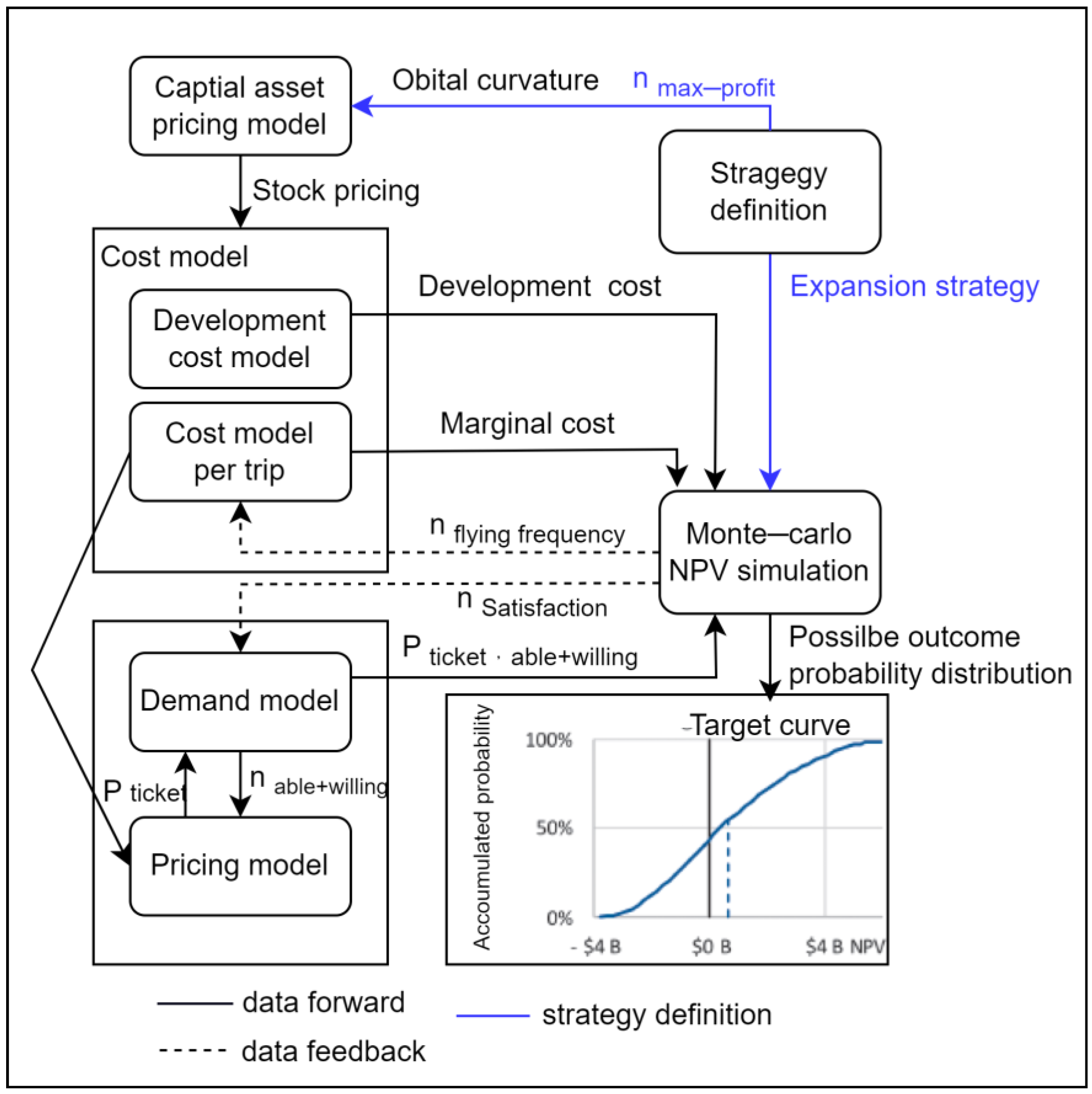
The space travel pricing model can be demonstrated in Figure 7. Its ticket price fluctuates are due to its bidding pricing strategy, which is concerned with cost models like spaceship design, drafting, engineering, manufacturing, labor, margin, and development costs. Demand conditions, like tourists’ financial capability and physical health, are also the parameters of the possible outcome of the pricing system. It can be summarized that the space travel pricing model is a complicated system that has been realized in the case of Virgin Galactic based on mathematics, economics, and computing implementation.

4.3. Discussions

4.3.1. Supply Side: The Supply Capability of Attaining Space Curvatures

At the beginning of commercial space travel, the pricing strategy was primarily dominated by suppliers, which means that consumers were price takers due to over-demand. Space travel can be dealt with only when the supplier invests the space capital to achieve a specific space curvature. The space supplier should integrate the fundings of liabilities and equity of the accounting Equation (2) to develop its space capital and achieve the production factors of space in Equation (1). The accounting cycle implies that, first, the incremental cash flows from the pricing strategy can be regarded as an incremental element of the energy–momentum tensor to attain the incremental spacetime curvature, the Einstein tensor. Second, the successful space launch and travel service then generate the equity premium due to the expected returns of investors. Third, the equity premium will raise the bidding price to increase the supplier’s profits, which will carry forward to the next period when the accounting cycle is completed. Fourth, incremental equity enlarges the size of capital assets to sustain the accounting cycle. The accounting cycle continues to increase the amounts of the accounting Equation (2) until the competition of other competitors offsets the equity premium. Thus, space travel pricing reflects the attainable curvature of the supplier’s capital investment, which supports Proposition 1.

4.3.2. Demand Side: Space Travel Value-at-Risk Investment

One of the characteristics of space travel is its high-risk attribute, similar to adventure tourism, with similar target market customers. These risk lovers prefer risky products, such as the extreme sports tourism market. However, risk-lover travelers have different risk tolerances and preferences; for example, travelers who would prefer to climb the world’s highest mountain peak are not the same as those who travel to space. No matter what kind of risk lover, the demand utility can typically be measured by value-at-risk (VaR), which determines the potential or probability of loss in the assessed entity. VaR can also be written as a distortion risk measure given by the distortion function [58], as shown in Equation (4).

$$gx=\left\{\begin{array}{c}0 if 0\le x<1-\alpha \\ 1 if 1-\alpha \le x\le 1\end{array}\right.\mathrm{The} \mathrm{VaR} \mathrm{at} \mathrm{level} \alpha \in \left(\mathrm{0,1}\right)$$

(6)

It can be implied that a space traveler is considered to be an investor who will lose their spending on space travel at the condition of g(x) = 0 in Equation (6), implying that a space journey purchase is a loss-inducing investment. The VaR model can assess the investment. The VaR investment from consumers becomes the supplier’s incremental equity. This will cause equity premium for value-added capital that helps the supplier to invest its space capital to attain the space curvatures. This is a pricing model where the demand side pays the price to support the supply side in achieving the expected space curvatures that support Proposition 2.

4.3.3. Market Equilibrium: Spacetime Equilibrium

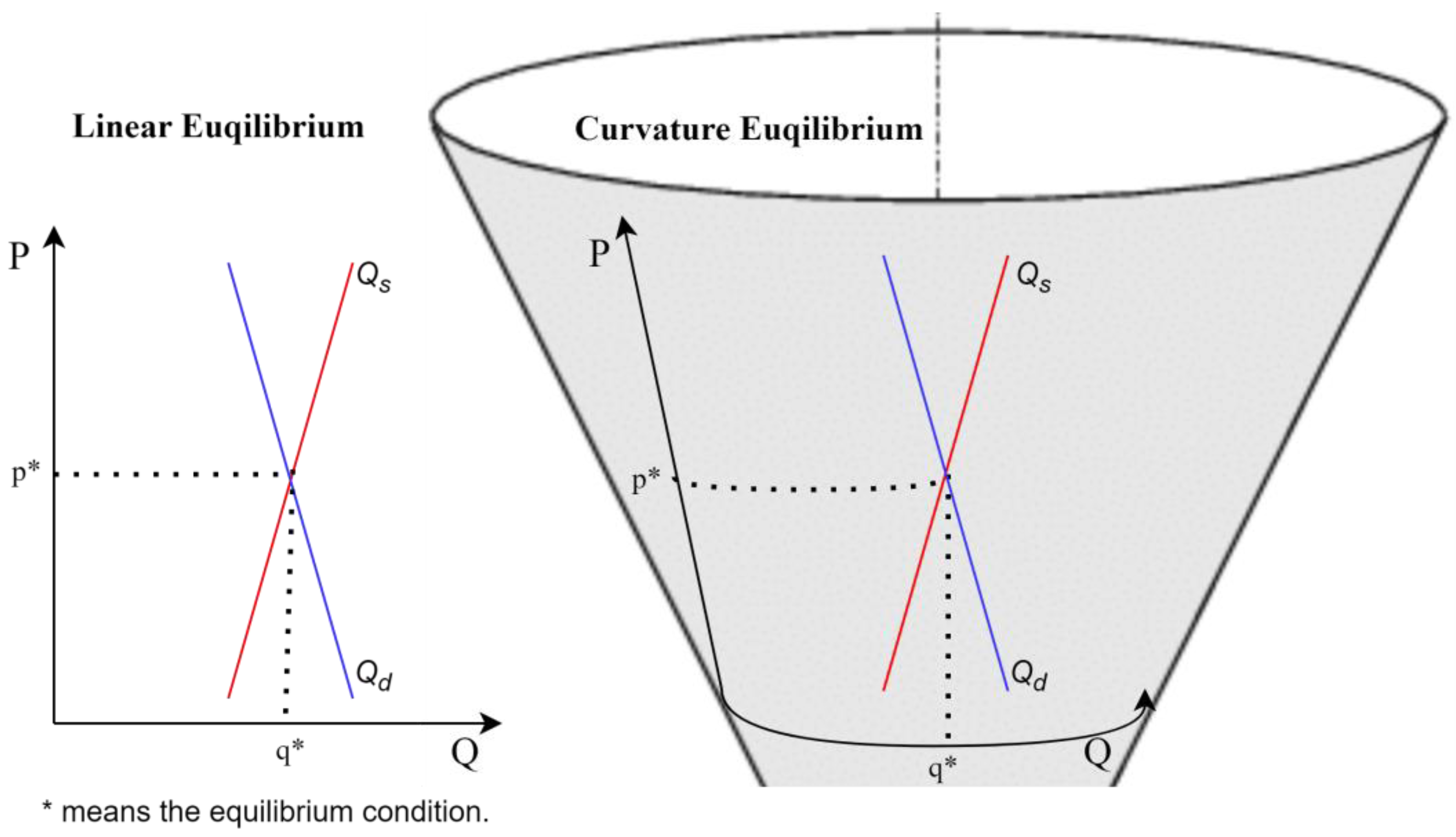
Based on the prerequisites of Equations (1)–(5), this study infers the space travel pricing model to the economic supply and demand reflected in the economic market equilibrium. The energy–momentum tensor provided by suppliers’ space capital can satisfy space travelers’ requirements to reach specific spacetime curvatures. On the supply side, suppliers are willing and able to invest space capital into the spacetime curvature, matching the energy–momentum tensor of the orbital altitude. On the demand side, there is a price that consumers are willing and able to pay for a particular spacetime curvature to meet their space travel requirement. Market equilibrium occurs when supply and demand both agree with the price that meets the expected spacetime curvature of space travel. However, we should convert the supply and demand from the traditional three-dimensional time- and space-independent framework into the spacetime four-dimensional framework. Notably, the market equilibria of Earth and space tourism differ. The space travel market equilibrium attains a curvilinear demand and supply intersection, which causes the difference in pricing models between Earth and space travel, as shown in Figure 8 [1]. We can examine space travel behaviors through interdisciplinary collaboration and test the research propositions and hypotheses to construct a space travel knowledge system. For example, testing the hypotheses from Propositions 1 and 2 can reveal the difference between space and Earth tourism through interdisciplinary models and artificial intelligence (AI) simulations.

5. Conclusions

5.1. Conclusions

This study logically applies the mathematical principles of GRT, the accounting equation, economic functions, and a computing algorithm to deduce the space travel pricing model according to the economic supply, demand, and market equilibrium behaviors. GRT has been generalized by many empirical studies in physics and cosmology. This study applies GRT to infer space travel economic behaviors, especially pricing behavior. The results showed that the geometric tensor equals the energy–momentum tensor of GRT, which can be analogically reasoned to the axiomatic set theory of the accounting equation: assets equal liability plus owner’s equity. The accounting equation presents capital investment as a space production factor for space travel products. Space travel pricing responds to a firm’s stock price regarding its capital investment returns. In addition, the demand side’s consumption function can be assumed as a VaR investment to echo the supplier’s production function. The maximum Walrasian Prices are then deducted to convey the commitment to market equilibrium. In summary, the space travel pricing mechanism is still guided by the invisible hand of market equilibrium, following supply and demand behaviors; however, the spacetime tensor must be transformed in the production factor and pricing model, which differs from the Earth market equilibrium.

The space travel pricing adjustment process is the inequality of the accounting equation that happens because of the equity premium effect on the capital investment of the space factor in a short period. However, the accounting equation will remain equal after the completion of the accounting cycle due to the incremental cash flows from revenue becoming the incremental equity. The equity premium caused by capital investment has a short-term effect on the accounting equation in advance. The net income will still be brought forward as the increment in equity, resulting in fixed-term equality of the accounting equation, which will be equal on both sides, like the GRT math equation. The capital investment injects the energy–momentum tensor required to achieve a specific curvature of space. On the demand side, space travel pricing assumes that a consumer spends on a VaR investment, and this consumption investment will echo the supply side’s accounting equation sets. Thus, we can conclude that space travel pricing remains the result of an economic market equilibrium between supply and demand based on the transactions that have been dealt with. The scientific invariant still applies to space economic behaviors, even though there are differences between space and Earth tourism.

5.2. Research Limitations and Suggestions

Space travel is a nascent industry and a significant tourist attraction. The research limits come from the availability of empirical data because the market is still immature, with few data. After enough space trips with empirical studies, this study’s results will respond more to market behaviors. At the same time, spacetime-related theories have to be developed to explain the reality of space economic behaviors to implement the four-dimensional spacetime tensor. The research directions of innovative fields can be studied from Earth to space, from independent space and time to integrated spacetime scales, from financial random walk to incremental random walk, and from referential time series to proper time series analyses. These innovative theories will bring about a new scientific vision when we conduct studies in the space market. For example, compared to a proper time series analysis, the traditional time series would present a higher risk because of significant fluctuations. It is one of the market abnormalities that await exploration from researchers in space studies.

Interdisciplinary theory construction requires cross-domain understanding and interdisciplinary communication between scholars in different fields. However, the academic culture of each field is conservative with its academic terminologies and theories. Multidisciplinary cooperation is necessary for innovative scientific theories. Moreover, scholars’ in-person cross-domain learning and research in different fields are more creative and effective in making breakthroughs. This study conducted analogical reasoning between the GRT of physics, economics, and computer science, connecting the three fields through econophysics methodology. However, more mathematical inference is needed to explore the physical connotation.

To sum up, space tourism is a nascent industry, and space travel lacks extensive empirical data, which could limit the immediate applicability of the pricing model. The interdisciplinary nature and the mathematics involved might make the model challenging to understand and apply for practitioners unfamiliar with GRT or econophysics. Moreover, the model’s accuracy depends on the validity of its assumptions regarding market behavior and the equivalence between economic principles and GRT, which might not hold under all commercial circumstances. The model’s focus on space travel pricing might limit its generalizability to other sectors or economic phenomena.

References

1. Peng, K.-L.; Hsu, C.H.C.; Lin, P.M.C.; Su, M. Proposing spacetime scale for space tourism economics. Tour. Econ. 2023, 29, 1671–1678. [Google Scholar] [CrossRef]
2. Lampkin, J.; White, R. The Global Space Industry. In Space Criminology: Analysing Human Relationships with Outer Space; Springer: Berlin/Heidelberg, Germany, 2023; pp. 25–47. [Google Scholar]
3. Olya, H.G.T.; Han, H. Antecedents of space traveller behavioral intentions. J. Travel Res. 2020, 59, 528–544. [Google Scholar] [CrossRef]
4. Dileep, M.R.; Pagliara, F. Space Tourism. In Transportation Systems for Tourism; Springer: Berlin/Heidelberg, Germany, 2023; pp. 269–288. [Google Scholar]
5. Wu, E.T. What Are the Truths of Gravity and General Relativity. IOSR J. Appl. Phys. (IOSR-JAP) 2022, 14, 25–51. [Google Scholar]
6. Perlov, D.; Vilenkin, A.; Perlov, D.; Vilenkin, A. The Fabric of Space and Time. In Cosmology for the Curious; Springer: Cham, Switzerland, 2017; pp. 59–82. [Google Scholar] [CrossRef]
7. Penprase, B.E. Spacetime and Curved Space. In Models of Time and Space from Astrophysics and World Cultures; Springer: Berlin/Heidelberg, Germany, 2023; pp. 129–161. [Google Scholar]
8. May, A. The Space Business: From Hotels in Orbit to Mining the Moon—How Private Enterprise is Transforming Space; Icon Books: London, UK, 2021. [Google Scholar]
9. Luo, S.; Song, F. Principles-based versus rules-based: Accounting standards precision and financial restatements in China. Asian Rev. Account. 2022, 30, 581–615. [Google Scholar] [CrossRef]
10. Juárez, F. The accounting equation inequality: A set theory approach. Glob. J. Bus. Res. 2015, 9, 97–104. [Google Scholar]
11. Carroll, S.M. Spacetime and Geometry; Cambridge University Press: Cambridge, UK, 2019. [Google Scholar]
12. Rodal, J.J. A Machian wave effect in conformal, scalar–tensor gravitational theory. Gen. Relativ. Gravit. 2019, 51, 64. [Google Scholar] [CrossRef]
13. Dolan, B.P. Einstein’s General Theory of Relativity: A Concise Introduction; Cambridge University Press: Cambridge, UK, 2023. [Google Scholar]
14. Barukčić, I. Unified field theory. J. Appl. Math. Phys. 2016, 4, 1379. [Google Scholar] [CrossRef]
15. Wu, J.; Xu, Y.; Bai, Q. Introduction to Space Science; Springer: Berlin/Heidelberg, Germany, 2021. [Google Scholar]
16. Simplício, P.; Marcos, A.; Bennani, S. Reusable launchers: Development of a coupled flight mechanics, guidance, and control benchmark. J. Spacecr. Rocket. 2020, 57, 74–89. [Google Scholar] [CrossRef]
17. Seo, B.R. Future of space travel. In Space Travel for the Masses: History, Current Status, Problems, and Future Directions; Worcester Polytechnic Institute: Worcester, MA, USA, 2013. [Google Scholar]
18. Kimmel, P.D.; Weygandt, J.J.; Kieso, D.E. Financial Accounting: Tools for Business Decision-Making; John Wiley & Sons: Hoboken, NJ, USA, 2020. [Google Scholar]
19. Prasad, S.; Green, C.J.; Murinde, V. Company Financing, Capital Structure, and Ownership: A Survey, and Implications for Developing Economies; SUERF Studies: New York, NY, USA, 2001. [Google Scholar]
20. Juárez, F. The foundations of balance sheet and the inequality of the basic accounting equation from the viewpoint of set theory. In Global Conference on Business & Finance Proceedings; Institute for Business & Finance Research: Hilo, HI, USA, 2015. [Google Scholar]
21. Conti, L. Russell’s paradox and free zig zag solutions. Found. Sci. 2023, 28, 185–203. [Google Scholar] [CrossRef]
22. Ludwig, W. Tractatus Logico-Philosophicus; Akadémiai Kiadó: Budapest, Hungary, 1989. [Google Scholar]
23. Makridis, O. Basics of Set Theory. In Symbolic Logic; Springer: Berlin/Heidelberg, Germany, 2022; pp. 405–458. [Google Scholar]
24. Okuyama, Y.; Chang, S.E. Modeling Spatial and Economic Impacts of Disasters; Springer Science & Business Media: Berlin/Heidelberg, Germany, 2004. [Google Scholar]
25. Johnson, H.G. The neo-classical one-sector growth model: A geometrical exposition and extension to a monetary economy. Economica 1966, 33, 265–287. [Google Scholar] [CrossRef]
26. Swan, P.L. Is Investment Into Infrastructure Needed to Achieve Affordable Space Launch? ASCEND: Las Vegas, NV, USA, 2023; p. 4604. [Google Scholar]
27. Mirman, L.J. The steady state behavior of a class of one sector growth models with uncertain technology. J. Econ. Theory 1973, 6, 219–242. [Google Scholar] [CrossRef]
28. Tohamy, S.M.; Mixon, J.W., Jr. Illustrating consumer theory with the CES utility function. J. Econ. Educ. 2004, 35, 251–258. [Google Scholar]
29. Morrell, P.S. Airline Finance; Routledge: London, UK, 2021. [Google Scholar]
30. Van Benthem, J.; Girard, P.; Roy, O. Everything else being equal: A modal logic for ceteris paribus preferences. J. Philos. Log. 2009, 38, 83–125. [Google Scholar] [CrossRef]
31. Chen, X. Cosmic Inquiries; Columbia University: New York, NY, USA, 1999. [Google Scholar]
32. Renn, J. The Genesis of General Relativity: Sources and Interpretations; Springer Science & Business Media: Berlin/Heidelberg, Germany, 2007; Volume 250. [Google Scholar]
33. Cyril, U.M.; Echobu, O.J.; Chukwuemeka, M.C. Evaluation of the Effect of Financial Factors on Shareholders’ Value of Listed Pharmaceutical Firms in Nigeria. Int. J. Financ. Bank. Res. 2019, 5, 114–125. [Google Scholar] [CrossRef]
34. Liu, Z.; Gao, R.; Zhou, C.; Ma, N. Two-period pricing and strategy choice for a supply chain with dual uncertain information under different profit risk levels. Comput. Ind. Eng. 2019, 136, 173–186. [Google Scholar] [CrossRef]
35. Alaagam, A. The relationship between profitability and stock prices: Evidence from the Saudi banking sector. Res. J. Financ. Account. 2019, 10, 91–101. [Google Scholar]
36. Capoani, L. Theory of Commercial Gravitational Fields in Economics: The Case of Europe. Netw. Spat. Econ. 2023, 23, 845–884. [Google Scholar] [CrossRef]
37. Savoiu, G.; Siman, I.I. History and role of econophysics in scientific research. In Econophysics: Background and Applications in Economics, Finance, and Sociophysics; Academic Press: Cambridge, MA, USA, 2013; pp. 3–16. [Google Scholar]
38. Săvoiu, G. Statistical thinking and statistical Physics. In Proceedings of the International Conference Econophysics, New Economics & Complexity, Hyperion University and Hyperion Research & Development Institute, Bucharest, Romania, 22 February 2008; Victor Publishing House: Bucharest, Romania, 2008; pp. 85–99. [Google Scholar]
39. Savoiu, G.; Andronache, C. The potential of econophysics for the study of economic processes. In Econophysics Background and Applications in Economics, Finance, and Sociophysics; Academic Press: Cambridge, MA, USA, 2013; pp. 91–133. [Google Scholar]
40. Morales-Bañuelos, P.; Muriel, N.; Fernández-Anaya, G. A Modified Black-Scholes-Merton Model for Option Pricing. Mathematics 2022, 10, 1492. [Google Scholar] [CrossRef]
41. Rickles, D. Econophysics and the complexity of financial markets. In Philosophy of Complex Systems; Elsevier: Amsterdam, The Netherlands, 2011; pp. 531–565. [Google Scholar]
42. Phlips, L. The Economics of Price Discrimination; Cambridge University Press: Cambridge, UK, 1983. [Google Scholar]
43. Müller, C.; Gönsch, J.; Soppert, M.; Steinhardt, C. Customer-centric dynamic pricing for free-floating vehicle sharing systems. Transp. Sci. 2023, 57, 1406–1432. [Google Scholar] [CrossRef]
44. Klainerman, S.; Szeftel, J. Global Nonlinear Stability of Schwarzschild Spacetime under Polarized Perturbations:(AMS-210); Princeton University Press: Princeton, NJ, USA, 2020; Volume 210. [Google Scholar]
45. Ariely, D.; Simonson, I. Buying, bidding, playing, or competing? Value assessment and decision dynamics in online auctions. J. Consum. Psychol. 2003, 13, 113–123. [Google Scholar] [CrossRef]
46. Cosgrove, J.K. Einstein’s Principle of Equivalence and the Heuristic Significance of General Covariance. Found. Phys. 2021, 51, 27. [Google Scholar] [CrossRef]
47. Guruswami, V.; Hartline, J.D.; Karlin, A.R.; Kempe, D.; Kenyon, C.; McSherry, F. On Profit-Maximizing Envy-Free Pricing; SODA: Vancouver, Canada, 2005. [Google Scholar]
48. Chalermsook, P.; Chuzhoy, J.; Kannan, S.; Khanna, S. Improved hardness results for profit maximization pricing problems with unlimited supply. In International Workshop on Approximation Algorithms for Combinatorial Optimization; Springer: Berlin/Heidelberg, Germany, 2012. [Google Scholar]
49. Bucarey, V.; Elloumi, S.; Labbé, M.; Plein, F. Models and algorithms for the product pricing with single-minded customers requesting bundles. Comput. Oper. Res. 2021, 127, 105139. [Google Scholar] [CrossRef]
50. Fernandes, C.G.; Ferreira, C.E.; Franco, Á.J.; Schouery, R.C. The envy-free pricing problem and unit-demand markets. In International Symposium on Combinatorial Optimization; Springer: Berlin/Heidelberg, Germany, 2014. [Google Scholar]
51. Fernandes, C.G.; Ferreira, C.E.; Franco, Á.J.; Schouery, R. The unit-demand envy-free pricing problem. arXiv 2013, arXiv:1310.0038. [Google Scholar] [CrossRef]
52. Gul, F.; Stacchetti, E. Walrasian equilibrium with gross substitutes. J. Econ. Theory 1999, 87, 95–124. [Google Scholar] [CrossRef]
53. Bosch Martínez, A. Study of the Benefits and Applications of Passenger Supersonic Transport Vehicles: Case Study of Supersonic 2.0-Virgin Galactic. Bachelor’s Thesis, Universitat Politècnica de Catalunya, Barcelona, Spain, 2023. [Google Scholar]
54. Madan, B.; Halkias, D. Emancipated entrepreneurship in the European space sector: The case of Richard Branson’s Virgin Galactic as a driver of space tourism. SSRN Electron. J. 2020. [Google Scholar] [CrossRef]
55. Giachino, C.; Pucciarelli, F.; Bollani, L.; Bonadonna, A. Is Generation Z ready to fly into the space? The future of tourism is coming. Futures 2023, 145, 103064. [Google Scholar] [CrossRef]
56. Musselman, B.T.; Winter, S.R.; Rice, S.; Keebler, J.R.; Ruskin, K.J. Point-to-point suborbital space tourism motivation and willingness to fly. Ann. Tour. Res. Empir. Insights 2024, 5, 100119. [Google Scholar] [CrossRef]
57. Sheetz, M. The down to earth guide to investing in space. In Expanding Frontiers; Brown, G., Ed.; UK Space Agency: Swindon, UK, 2023; pp. 1–27. [Google Scholar]
58. Sepanski, J.H.; Wang, X. New Classes of Distortion Risk Measures and Their Estimation. Risks 2023, 11, 194. [Google Scholar] [CrossRef]
Figure 1. The spacetime curvature and matter movement.
Mathematics 12 00757 g001
Figure 2. The spacetime production function.
Mathematics 12 00757 g002
Figure 3. The space travel pricing process.
Mathematics 12 00757 g003
Figure 4. Analogy method.
Mathematics 12 00757 g004
Figure 5. Space travel prices at different altitudes.
Mathematics 12 00757 g005
Figure 6. SPCE share price fluctuation after the month routine flies of Virgin Galactic.
Mathematics 12 00757 g006
Figure 7. The bidding pricing model of Virgin Galactic.
Mathematics 12 00757 g007
Figure 8. Economic equilibria of time and spacetime references.
Mathematics 12 00757 g008
Disclaimer/Publisher’s Note: The statements, opinions and data contained in all publications are solely those of the individual author(s) and contributor(s) and not of MDPI and/or the editor(s). MDPI and/or the editor(s) disclaim responsibility for any injury to people or property resulting from any ideas, methods, instructions or products referred to in the content.