Deep Graph Learning-Based Surrogate Model for Inverse Modeling of Fractured Reservoirs

Abstract

Inverse modeling can estimate uncertain parameters in subsurface reservoirs and provide reliable numerical models for reservoir development and management. The traditional simulation-based inversion method usually requires numerous numerical simulations, which is time-consuming. Recently, deep learning-based surrogate models have been widely studied as an alternative to numerical simulation, which can significantly improve the solving efficiency of inversion. However, for reservoirs with complex fracture distribution, constructing the surrogate model of numerical simulation presents a significant challenge. In this work, we present a deep graph learning-based surrogate model for inverse modeling of fractured reservoirs. Specifically, the proposed surrogate model integrates the graph attention mechanisms to extract features of fracture network in reservoirs. The graph learning can retain the discrete characteristics and structural information of the fracture network. The extracted features are subsequently integrated with a multi-layer recurrent neural network model to predict the production dynamics of wells. A surrogate-based inverse modeling workflow is then developed by combining the surrogate model with the differential evolutionary algorithm. Numerical studies performed on a synthetic naturally fractured reservoir model with multi-scale fractures illustrate the performance of the proposed methods. The results demonstrate that the proposed surrogate model exhibits promising generalization performance of production prediction. Compared with tens of thousands of numerical simulations required by the simulation-based inverse modeling method, the proposed surrogate-based method only requires 1000 to 1500 numerical simulations, and the solution efficiency can be improved by ten times.

1. Introduction

Fluid flow in fractured reservoirs is significantly influenced by the distribution of fractures. Hence, it is necessary to accurately estimate the fracture distribution for the simulation and management of fractured reservoirs [1]. Inverse modeling, also termed history matching in petroleum engineering, is an effective method for predicting the distribution of fractures. Based on numerical simulation techniques, inverse modeling methods can estimate the uncertain parameters in numerical models by integrating geological information and production dynamics [2]. However, the simulation-based inverse modeling workflows require large numbers of numerical simulations, which can be computationally expensive [3]. Typically, a single numerical simulation of fractured reservoirs may consume minutes to hours of computer processing time.

To tackle this problem, surrogate-based inverse modeling methods utilize computationally cheap surrogate models to substitute the numerical simulations needed in inversion. Typically, surrogate models used in inverse modeling fall into three categories: physic-driven, data-driven, and hybrid ones. Considering the complex fluid flow mechanism of fractured reservoirs, data-driven surrogate models are often the method of choice. Hamid et al. [4] applied the Gaussian process model as the surrogate to assist the history matching of an unconventional gas reservoir. They estimated the coefficient of fluid composition in the numerical model, which is a 20-dimensional inverse problem. Dachanuwattana et al. [5] developed a surrogate-assisted inverse modeling method for shale reservoirs, and they compared the accuracy of quadratic polynomial, cubic polynomial, k-nearest neighboring, and kriging models. Their results showed that the kriging model has the best effect. Zhang and Sheng [6] also employed the kriging model as the surrogate for optimizing hydraulic fracturing in a naturally fractured shale reservoir. These surrogate models are based on traditional machine learning methods, which are suitable for low-dimensional problems. Therefore, it is necessary to select a small number of key features as input parameters before building the surrogate model.

Recently, deep-learning (DL)-based surrogate models have been widely studied for the inverse modeling of conventional reservoirs [7,8]. The essence of these DL-based surrogate models lies in the utilization of convolutional neural network (CNN) models to extract high-level features from spatially distributed parameters with a grid-like structure, such as the permeability field. Compared with traditional machine learning methods, DL-based models can directly learn features of high-dimensional parameters, which can avoid artificial feature selection as well as retaining more detailed information for prediction. However, unlike conventional reservoirs, fractured reservoirs are composed of fractures with discrete and irregular characteristics, which is difficult to be processed by conventional DL methods. Zhang et al. [9] employed a deep sparse autoencoder model to develop the re-parameterization method for the inverse modeling of fractured reservoirs. In this approach, a deep artificial neural network (ANN) model was utilized to capture the features of the complete geometry parameters of the fracture network. Chen et al. [10] adopted the variational auto-encoder and generative adversarial network to reduce the high-dimensional parameters of the fracture network to low-dimensional continuous parameters for the inversion modeling of fracture network. In their model, the geometric parameters of each fracture are combined into vector data for feature learning. Yan et al. [11] developed a CNN-based surrogate model for enhanced geothermal systems, and it can predict the temperature field and produced fluid temperature by using the continuous fracture permeability field. Kim and Durlofsky [12] proposed an DL-based surrogate model for production optimization of fractured reservoirs, in which they utilized the single-phase steady-state solution of the pressure equation to replace fracture network input into the CNN model. These studies have successfully applied deep learning methods to the inverse modeling or production optimization of fractured reservoirs with a complex fracture network. However, these methods need to transform the fracture network into continuous parameters or parameter fields for feature learning and ignore the discrete characteristics of fractures.

In this paper, we propose a deep graph learning-based surrogate model for the numerical simulation of fractured reservoirs with a multi-scale fracture network. The numerical simulation model adopted in this work is the embedded discrete fracture model (EDFM) [13,14], which is popular due to its ability to strike a balance between computational efficiency and accuracy. This new surrogate model is referred to as the GAT-LSTM, in which a graph attention (GAT) model [15,16] and an LSTM model [17,18] cooperatively emulate the EDFM simulation process. This surrogate model structure is similar to the convolutional recurrent neural network for the history matching of reservoirs [12,19]. Recently, deep graph learning methods [20,21,22] have garnered significant attention and research in the DL community. This is because deep graph learning methods can effectively address the challenge of feature learning in unstructured data, encompassing domains such as knowledge graphs [23], social networks [24], and protein structure prediction [25].

In summary, this work makes the following contributions:

(1)

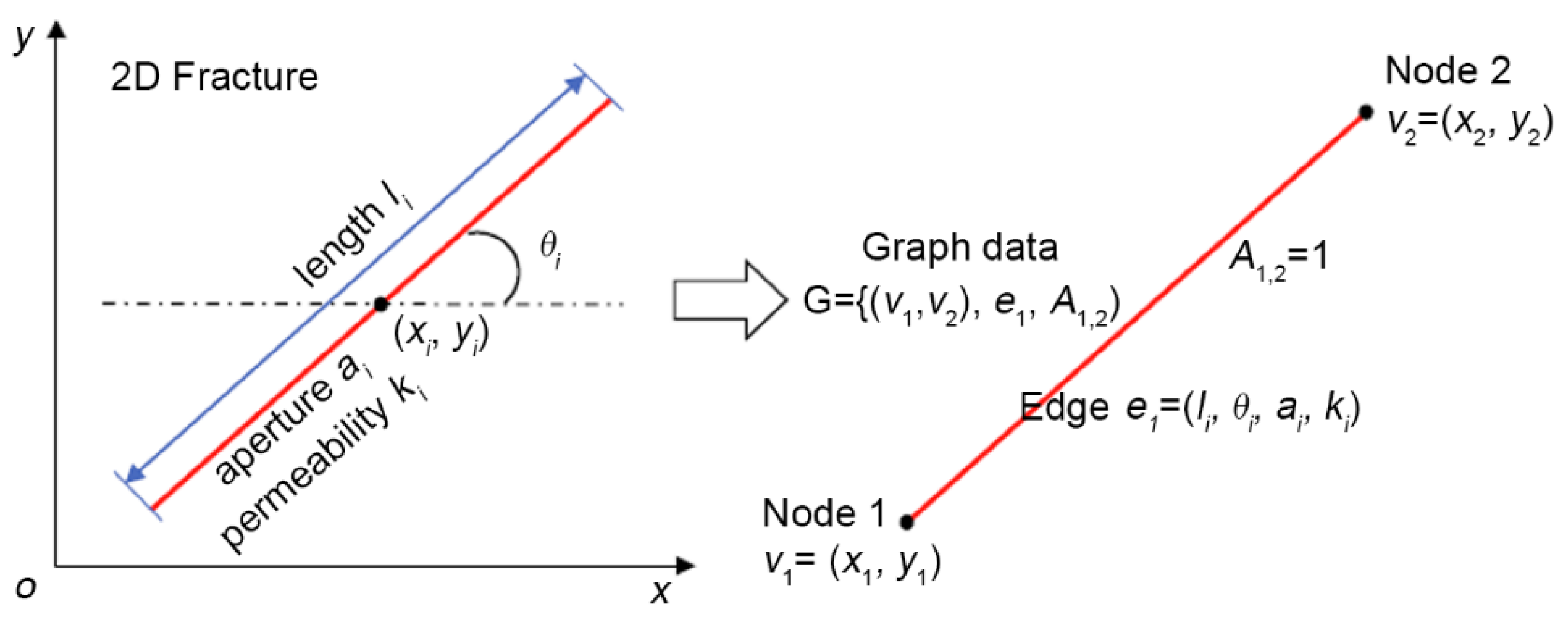
A novel deep graph learning-based feature learning method for the complex multi-scale fracture network is proposed. In this approach, the fracture network is represented as graph data, and the feature learning is performed based on parameters of each discrete fracture, which can effectively retain the discrete characteristics and geometric information of the fracture network. To the best of our knowledge, no work has reported using the deep graph learning method for the feature learning of a fracture network.

(2)

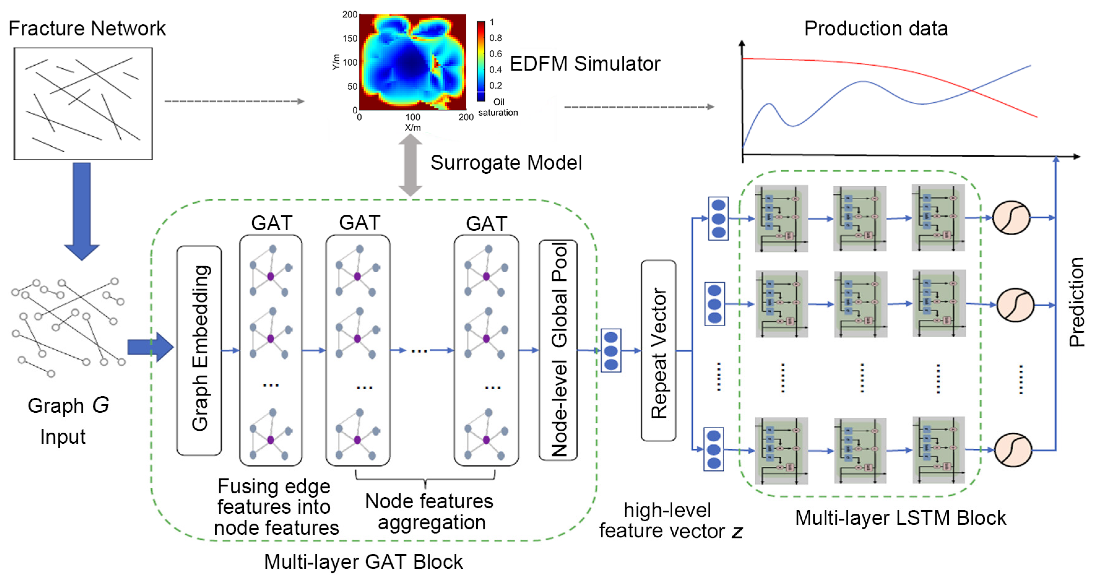
Based on the deep graph learning and multi-layer recurrent neural networks, a surrogate model for the embedded fracture numerical simulation was developed for the inversion of fracture distribution. This surrogate model can predict the production dynamics of wells under different fracture distribution conditions. Compared with EDFM simulation, the proposed surrogate model significantly reduces the computation cost of production prediction.

(3)

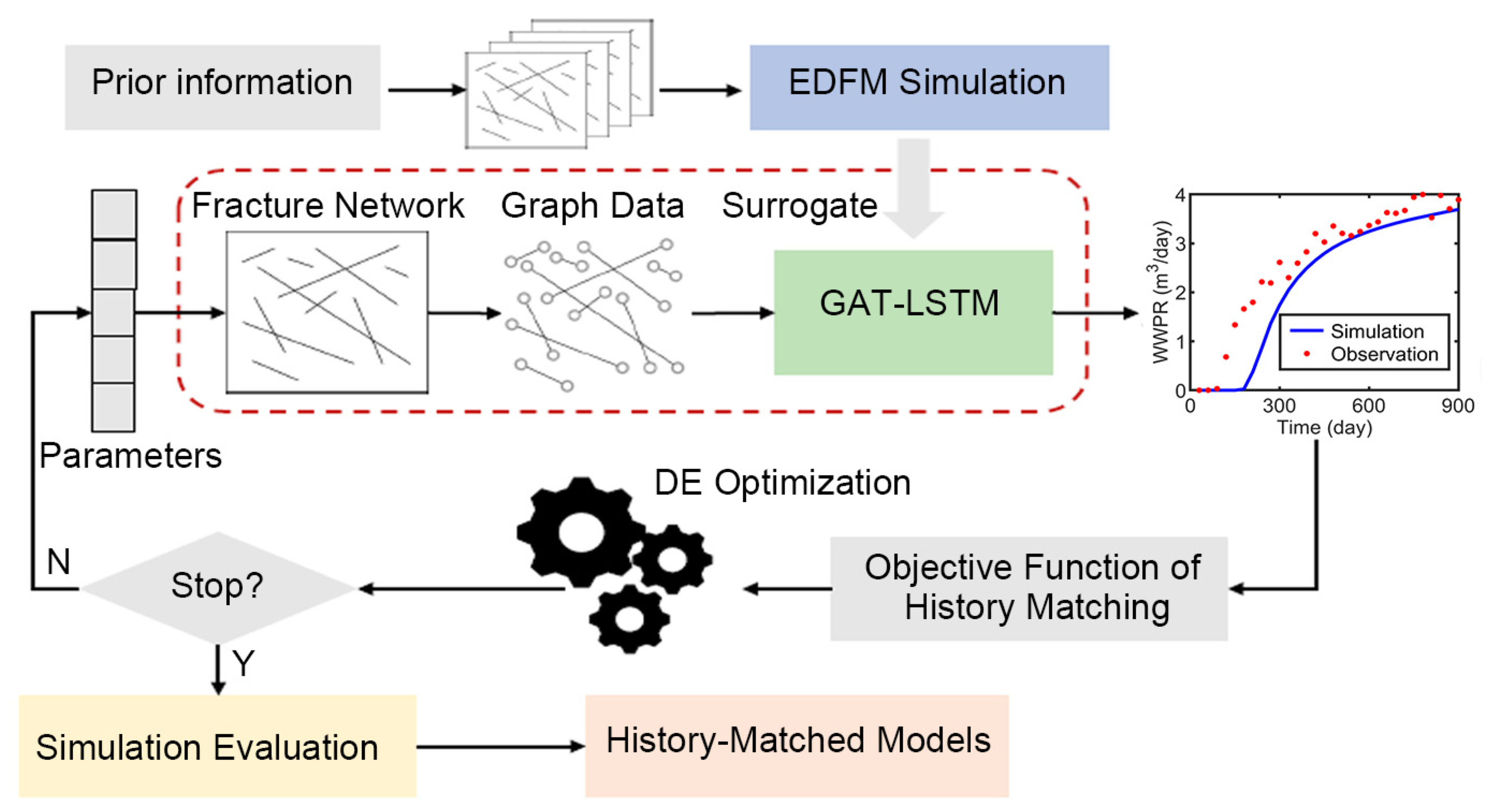
An effective surrogate-based inverse modeling framework was designed, which integrates the population-based differential evolution (DE) algorithm with the proposed surrogate model. Because of the cheap computational cost of the surrogate model, the search performance of the DE algorithm can be fully released and improve the solving efficiency of the inversion.

The remainder of the paper is organized as follows: Section 2 introduces the methods used in this study, including the generation method of the 2D multi-scale fracture network, the proposed GAT-LSTM surrogate model, and the surrogate-based inverse modeling workflow. Then, the surrogate model performance and inverse modeling results of a 2D fractured reservoir case are provided in Section 3. Finally, we conclude this work in Section 4 with a summary and mention of potential future work.

2. Methods

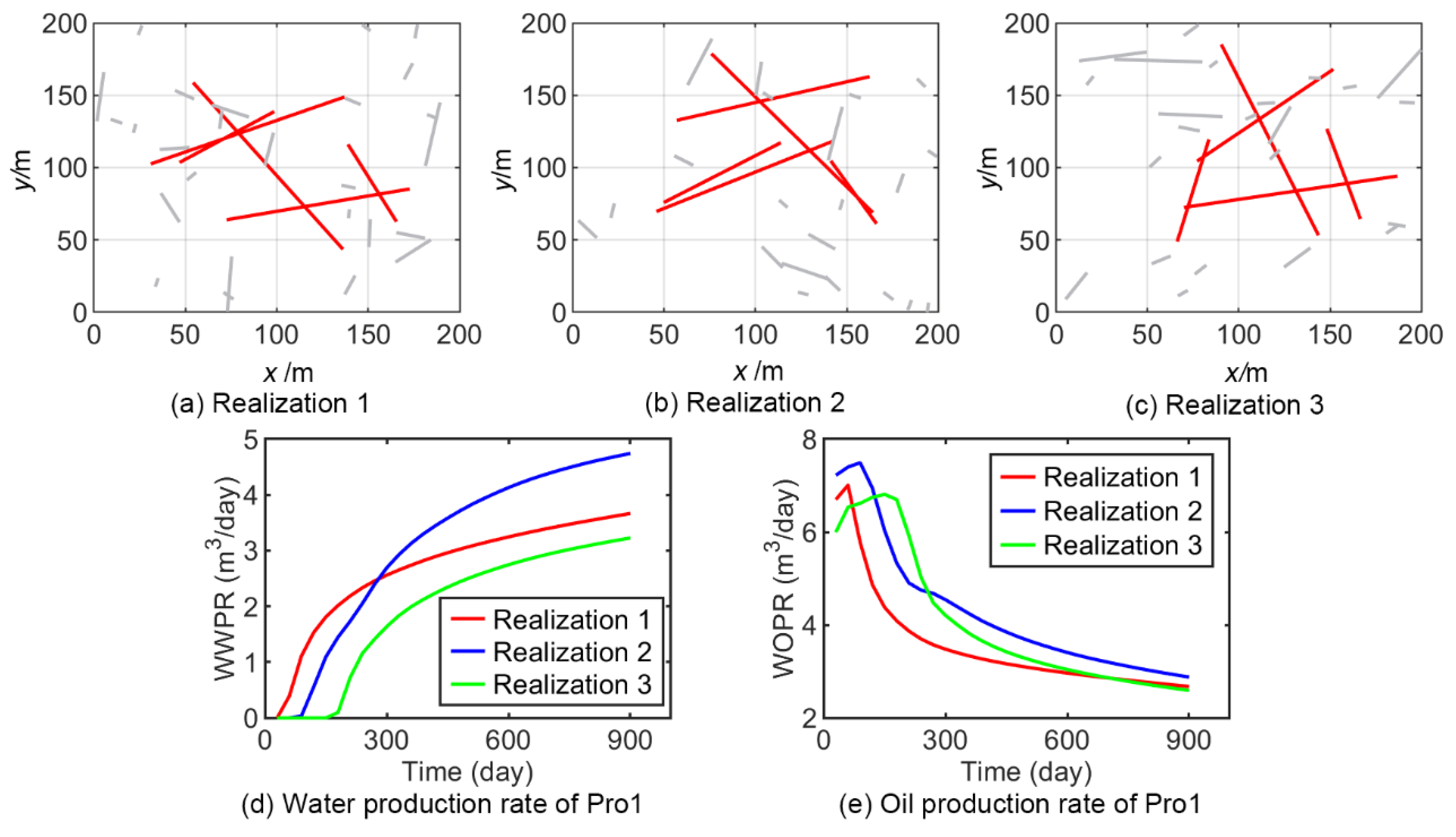
2.1. Generation of 2D Multi-Scale Fracture Network

Based on our previous work [26], a parameterization method integrating large-scale and small-scale fractures hierarchically was used to generate the 2D fracture network. First, the large fractures were characterized with the fracture length, orientation, and coordinates of the fracture center, while the small fractures were generated by using statistical modeling methods. The parameters of large fractures are characterized as:

$$m_l={\{x_i,y_i,{\theta }_i,l_i\}}_{i=1,2,\dots ,N_l}$$

(1)

where $m_l$ is the parameter vector of large fractures, $(x_i,y_i)$ is the midpoint coordinate of the $i\mathrm{th}$ large fracture, ${\theta }_i$ is the fracture orientation, $l_i$ is the fracture length, and $N_i$ is the number of large fractures. For naturally fractured reservoirs, the prior information of large fractures can be obtained by using measurements such as petrophysical interpretation, in situ stress data analysis, log data, and so forth [27].

Then, the small-scale fractures can be generated by using the statistical method. Specifically, we use the fractal-scaling law to generate the length, a normal distribution to generate the orientation, and a uniform distribution to generate the midpoint coordinates. The fracture network usually consists of multiple fracture sets with different statistical properties, assuming that there are $N_{set}$ fracture sets and the intensity $D_i$ of ith set. The intensity is defined as the ratio of the fracture number of the ith set to the total fracture number. The total number of small-scale fractures can be obtained by the fractal-scaling law. In order to describe the heterogeneity of fracture distribution in the reservoir area, we partitioned the reservoir into four sub-regions and established the proportion of the fracture number for each sub-region. This proportion is defined as the ratio of the fracture number in a sub-region to the total fracture number in the entire region. To facilitate the inversion, the proportional score $P_j\in [0.1,1]$ was used as the parameter, and the proportion can be computed by using the normalization of proportion scores. In conclusion, the small-scale fractures can be parameterized by using statistical parameters as follows:

$$m_s={\{D_l,D_i,{\theta }_i,{\sigma }_i,P_j\}}_{i=1,\dots ,N_{set}; j=1,\dots ,N_{re}}$$

(2)

where $m_s$ is the parameter vector of small fractures, $D_l$ is the fractal dimension of small fractures length, ${\theta }_i$ and ${\sigma }_i$ are the mean and standard deviation of orientation of ith fracture set, P_j is the proportion score of the jth sub-region.

The fracture network can be generated based on the parameter vectors $m_l$ and $m_s$. Meanwhile, the parameters $m_l$ and $m_s$ are used as uncertainty parameters in history matching to estimate the fracture distribution. Besides these parameters, the aperture and permeability of the fracture is also significant for fluid flow. According to the cubic law, we can calculate the permeability of the fracture with the aperture. The aperture of the fracture is related to the length. Equations (3) and (4) show the relation of the fracture permeability $k_f$, the aperture $a$, and the length $l$. The coefficient $c_a$ can be set between 10⁻¹ and 10⁻³ [28].

$$a=c_a\cdot l$$

(3)

$$k_f=a^2/12$$

(4)

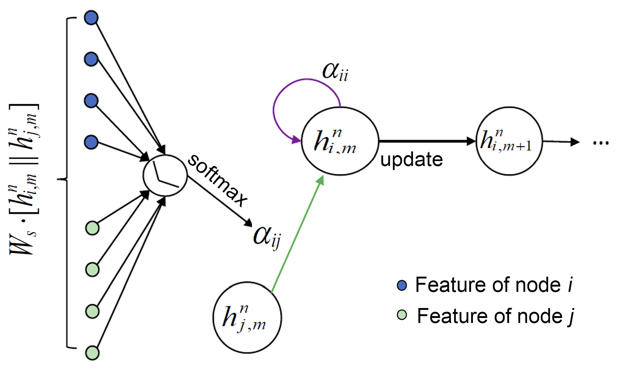
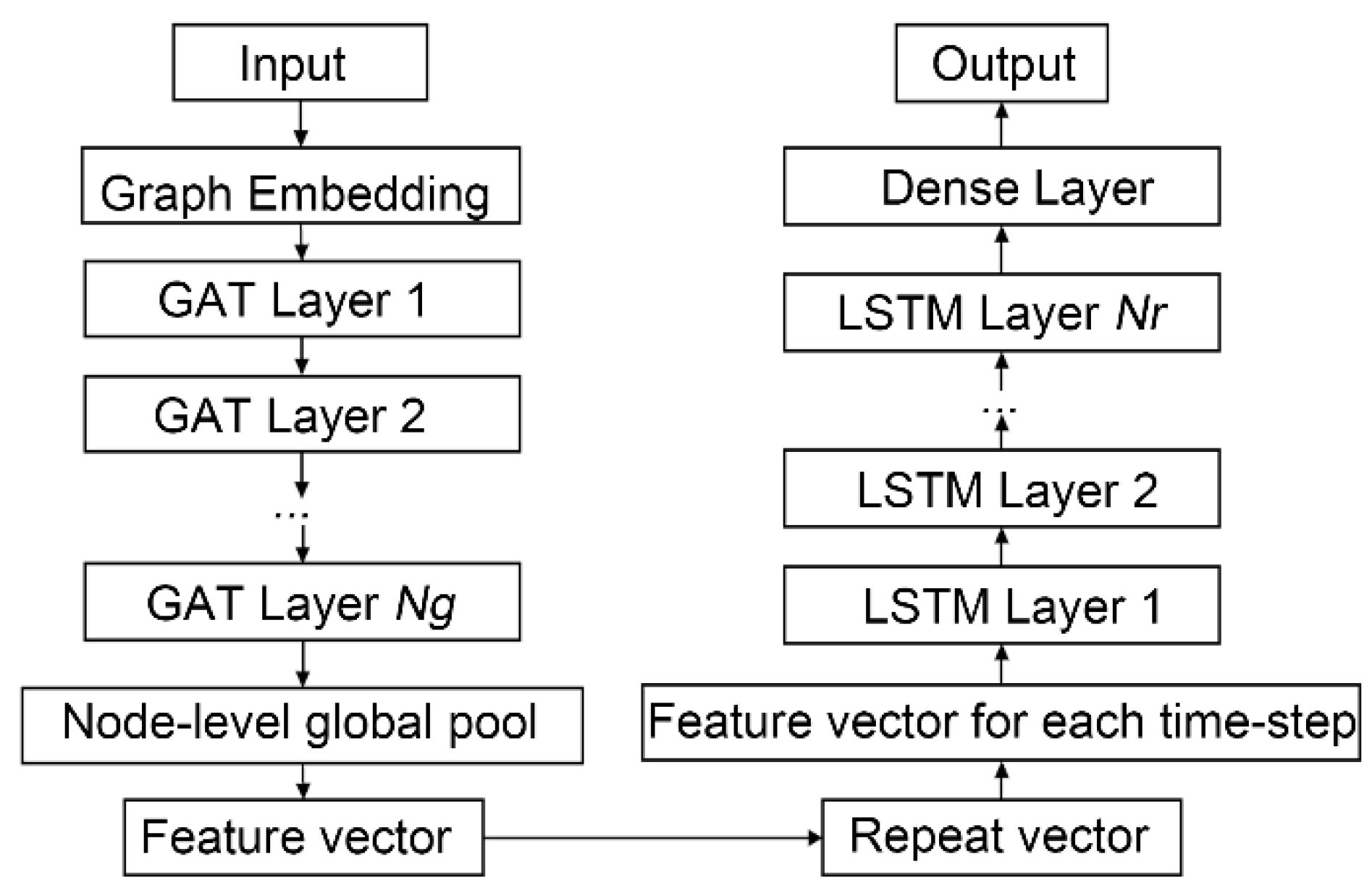
2.2. GAT-LSTM Surrogate Model

Given that uncertainty in the numerical model mainly arises from the geometry distribution of fractures, the relationship between the input and output in the EDFM simulation for history matching can be described as follows:

$$f:G\to Y\in R^{T\times N_d}$$

(5)

where G is the fracture network, Y is the flow response of simulation, T is the number of the time-step in the simulation, and N_d is the number of observation indicators, such as the water or oil production rate of different wells. The fracture network G consists of $N_f$ fractures with geometry and flow parameters.

The characterization of the fracture network G is based on properties of each fracture. Fractures are discontinuous in reservoir space. Therefore, the characterization of the fracture network is non-structural. Graph learning is an effective method to deal with unstructured data. For graph learning, we first need to represent the fracture network to the graph data $G=(V,E,A)$. As shown in Figure 1, there are $2N_f$ nodes and $N_f$ edges due to each fracture having two nodes (the endpoints of the fracture) and one edge, where the node set V includes the end coordinates of all fractures ${\{v_i=(x_i,y_i)\}}_{i=1,\dots ,2N_f}$, the edge set E includes the edge attribute ${\{e_i=(l_i,{\theta }_i,a_i,k_i)\}}_{i=1,2,\dots ,N_f}$, and $A\in {ℝ}^{2N_f\times 2N_f}$ is the adjacency matrix, $A_{ij}=1$ denotes the existing edge from node j to node i, otherwise, $A_{ij}=0$.

The surrogate model used to approximate such an input–output relationship can be transformed to a graph-to-sequence regression problem. Based on these findings, this paper introduces a deep graph learning-based surrogate model, termed GAT-LSTM. It integrates two key components: a graph representation learning block and a time series regression block, as illustrated in Figure 2. In the first block, based on the graph representation learning, we wish to learn an encoder to extract the high-level feature vector z from the fracture network G by using the GAT model. In the second block, the LSTM model is adopted to predict the flow response Y by using the feature vector z.

In order to obtain sufficient expressive power for transforming the fracture network G into high-level features, the graph representation learning block comprises a feature embedding layer and a multi-layer GAT model. The node and edge features consist of the location, length, angle, aperture, and permeability of the fracture;. these input features have different distributions and semantics. By using the embedding layer, the input information can map from a lower-dimensional heterogeneous space to a higher-dimensional homogeneous space, allowing the network to learn more about the relationship between inputs. In our model, the embedding layer is a single-layer feedforward neural network, parametrized by a weight matrix and applying the rectified linear unit (ReLU) activation function [29], as follows:

$$h_i^n=\mathrm{ReLU}(W_v\cdot v_i+b_v)$$

(6)

$$h_k^e=\mathrm{ReLU}(W_e\cdot e_k+b_e)$$

(7)

where $h_i^n\in {ℝ}^d$ is the embedding features of node $i$, $h_k^e\in {ℝ}^d$ is the embedding features of edge k, $d$ is the dimension of embedding features, which is a hyperparameters, $W_v$ and $b_v$ represent the weight parameters and bias term for node features. $W_e$ and $b_e$ represent the weight parameters and bias term for edge features.

Afterward, a multi-layer GAT model is constructed to learn the graph-level representation of fracture network from the node and edge embedding features. As shown in Figure 3, the single GAT layer consists of a learnable linear transformation parameterized by the weight matrix and a self-attention operation on nodes, which computes a learned weighted average of all of the neighbors’ features.

For the $m\mathrm{th}$ GAT layer, the attention score s between node i and its neighbor node $j\in {\mathcal{N}}_i$ is computed by using a multi-layer perceptron layer as follows:

$$s(h_{i,m}^n,h_{j,m}^n)=c^T\mathrm{LeakyReLU}(W_s\cdot [h_{i,m}^n\parallel h_{j,m}^n])$$

(8)

where ${\cdot }^T$ represents transposition and $\parallel$ is the concatenation operation, $c\in R^{2d^{\prime }}$ and $W_s\in {ℝ}^{2d^{\prime }\times 2d}$ are learned weight parameters, LeakyReLU [29] is the activation function, $d$ and $d^{\prime }$ are the dimensions of the inputs and outputs of the layer. These attention scores are normalized across all of $j\in {\mathcal{N}}_i$ using the SoftMax function to compute the attention coefficient:

$${\alpha }_{ij}=\mathrm{SoftMax}(s(h_{i,m}^n,h_{j,m}^n))=\frac{\exp (s(h_{i,m}^n,h_{j,m}^n))}{{\displaystyle {\sum }_{j^{\prime }\in {\mathcal{N}}_i}\exp (s(h_{i,m}^n,h_{j^{\prime },m}^n))}}$$

(9)

Then, the GAT layer computes a weighted average of the transformed features of the neighbor nodes as the new representation of node i, using the normalized attention coefficients:

$$h_{i,m+1}^n=\sigma ({\sum }_{j\in {\mathcal{N}}_i}{\alpha }_{ij}\cdot W_h{h}_{j,m}^n)$$

(10)

where $W_h\in {ℝ}^{d^{\prime }\times d}$ is the weight parameters, and $\sigma$ is the activation function. Equations (8)–(10) are one-time attention calculations and the multi-head attention is repeated w times. Hyperparameters of the GAT layer consists of dimension of output features $d$, number of heads $w$, and the activation function $\sigma$.

As shown in Figure 2, the multi-layer GAT block includes three steps: fusing the edge features into nodes, node features aggregation, and node-level global pool. The GAT layer mainly transforms node features through the connection relationship between nodes, so it is necessary to fuse edge features into nodes first. The feature fusion can be realized by propagating the features of edge $e_{i,j}$ to the corresponding nodes $i$ and $j$, and performing the GAT transformation. After that, GAT layers only need to aggregate the node features. Finally, all transformed node features are globally pooled to obtain the high-level feature vector z of the fracture network.

The extracted high-level feature vector z is utilized to predict the flow response data, which can be used as the input for each time-step of the multi-layer LSTM. The prediction of production data is a typical time series regression problem, the LSTM model can effectively solve this problem because of its recursive nature. For the time-series regression problem with T time-steps, the LSTM model requires $T$ basic units. To predict the observation data $Y=\{y_1,y_2,\dots ,y_T\}$, a stacked multilayer LSTM model is adopted in this work, as shown in Figure 2. The first LSTM layer receives input from extracted features of fracture network. Then, the input of the LSTM layer is the hidden state h from the layer. Generally, an LSTM model with 1 to 4 layers is recommended. Afterward, a time-distributed fully connected layer (the dense layer) is used to predict the production data. More details on multi-layer LSTMs can be found in our previous work [30]. To train the GAT-LSTM model, the mean absolute error (MAE) is used as the loss function, as follows:

$$J_{\beta }=\frac{1}{N}{\displaystyle {\sum }_{i=1}^N\left|y_i^{sim}-y_i^{pre}\right|}$$

(11)

where N is the size of evaluated samples, $y_i^{sim}$ and $y_i^{pre}$ are the numerical simulation results and surrogate prediction values, respectively. To evaluate the prediction performance of surrogate model, the coefficient of determination R² is adopted, which is defined as follows:

$$R^2=1-\frac{{\displaystyle {\sum }_{i=1}^N{\left|y_i^{sim}-y_i^{pre}\right|}^2}}{{\displaystyle {\sum }_{i=1}^N{\left|y_i^{sim}-y_m\right|}^2}}$$

(12)

where $y_m$ is the mean value of the numerical simulation results. The R² score provides a general estimate of the prediction performance. When the predicted result closely aligns with the simulation result, the R² score approaches 1.

Figure 4 summarizes the flowchart of the proposed GAT-LSTM model. In the first GAT layer, edge features are transferred to node features to achieve the fusion of edge features. The number of GAT layers Ng and the number of LSTM layers Nr are two hyperparameters of the model, which are set according to the specific reservoir simulation problem.

2.3. The GAT-LSTM Surrogate-Based Inverse Modeling Workflow

Figure 5 presents the proposed surrogate-based inverse modeling workflow for naturally fractured reservoirs, which consists of three phases. Firstly, initial realizations are generated by utilizing prior information, and a dataset is constructed using the EDFM numerical simulation for training the GAT-LSTM model. In this work, the EDFM simulation is conducted using the MATLAB reservoir simulation toolbox [31,32]. Secondly, the trained surrogate model is combined with the differential evolution (DE) algorithm to estimate uncertainty parameters and EDFM simulation is not necessary for this process. The uncertain parameters of the fracture network consist of geometry parameters, such as length, direction, and location, as well as some statistical parameters. The distribution of these uncertain parameters is non-Gaussian and high-dimensional, and the population-based DE algorithm is well-suited to handle such problems. Finally, the solutions obtained by DE are evaluated by EDFM simulation to obtain the final history-matched models. This step requires a small number of numerical simulations. In the following, we present the details of the history matching objective function and DE algorithm.

In order to estimate the fracture distribution, the history matching objective function can be defined as follows:

$$O(m)=-\frac{1}{2}{[d_{obs}-g(m)]}^T{C}_d^{-1}[d_{obs}-g(m)]$$

(13)

where $d_{obs}$ is the observation data, $g(\cdot )$ is the forward simulation, $m$ is the uncertainty parameter, and $C_d$ is the covariance of observation error. The detailed derivation of the objective function can be referred to previous studies [10,26]. In the surrogate-based inverse modeling workflow, the forward simulation is replaced with the surrogate model.

To minimize the objective function $O(m)$, the DE optimization algorithm is introduced. DE algorithm [33] finds optimal solutions of the objective function by evolving the differences between solutions in a population, and it performs well in dealing with nonlinear and high-dimensional optimization problems. The DE algorithm has three main operators: mutation, crossover, and selection. The mutation and crossover operations generate new solutions based on current solutions, as shown in Equations (14) and (15):

$$v_i^k=x_i^k+F_i\cdot (x_{best}^k-x_i^k)+F_i\cdot (x_{r1}^k-x_{r2}^k)$$

(14)

$$u_{i,j}^k=\{\begin{array}{l}{v}_{i,j}^k, \mathrm{if} \mathrm{rand}(0,1)\le C{R}_i \mathrm{or} j=jr\\ x_{i,j}^k, \mathrm{otherwise} \end{array}$$

(15)

where $v_i^k$ represent the $i\mathrm{th}$ mutant vector in the $k\mathrm{th}$ iteration, $x_i^k$ is the $i\mathrm{th}$ solution vector in current population, $x_{best}^k$ represents the best solution found in the $k\mathrm{th}$ iteration, $x_{r1}^k$ and $x_{r2}^k$ are two distinct solutions randomly selected from the current population, $u_{i,j}^k$ represents the $j\mathrm{th}$ dimension of the $i\mathrm{th}$ crossover vector $u$, and $F_i$ and $C{R}_i$ are the mutation factor and crossover probability, respectively.

After generating new solutions based on the mutation and crossover, the current population is updated through selection operations. For minimum problems, the selection operation is given by:

$$x_i^{k+1}=\{\begin{array}{l}{u}_i^k,\mathrm{if} o(u_i^k)<o(x_i^k)\\ x_i^k,\mathrm{otherwise} \end{array}$$

(16)

where $o(\cdot )$ represents the objective function. The above procedure is repeated until the terminal condition is satisfied, such as the maximum number of iterations being reached.

3. Case Studies

To investigate the prediction performance of the proposed GAT-LSTM surrogate model, we perform case studies on a synthetic 2D naturally fractured reservoir. In order to verify the feature learning ability of the GAT method for fracture networks, an ANN-LSTM surrogate model which uses the ANN model as feature extractor is compared. As a basic machine learning method, the ANN model has been widely used in data processing and surrogate modeling tasks. In this comparison, the ANN and GAT models use the same fracture network parameters to learn and extract features. The difference is that the GAT model can consider discrete characteristics and structure information of fracture network. Specifically, parameters such as location and length of all fractures in a fracture network are flattened into the input vector for the ANN model, and the zero-filling strategy is used to solve the size change in the input vector caused by the different number of fractures in a different fracture network. For the ANN-LSTM model, the maximum and minimum normalization method is used for input parameters. For the GAT-LSTM model, the input parameters are transformed by graph embedding, so no normalization is required. For production data, the log-transformation-based normalization method [30] is used.

Table 1. GAT-LSTM and ANN-LSTM architecture for the case studies. The d is number of neural units, t is number of time-steps, w is the number of heads.

Component	Layers	Hyper Parameters
Multi-layer GAT Block	Graph Embedding	d = 128, σ = ReLU
	GAT Layer 1/2/3/4	d = 128, w = 3, σ = ReLU
	Node-level Global Pool	Max pool
Multi-layer ANN Block	Dense Layer 1	d = 256, σ = ReLU
	Dense Layer 2	d = 128, σ = ReLU
	Dense Layer 3	d = 100, σ = ReLU
Multi-layer LSTM Block	Repeat Vector	t = 30
	LSTM Layer 1	d = 100
	LSTM Layer 2	d = 100
	Dense Layer 4	d = 8, σ = tanh

shows detailed configurations of the GAT-LSTM and ANN-LSTM models used in this experiment. The neural network model is implemented on the TensorFlow platform [34], and graph learning is realized using the TensorFlow Graph Neural Networks library [35]. All models are trained on a single NVIDIA GeForce RTX 3090 GPU with 24 GB memory. The Adam algorithm [36] was employed as the optimizer, with an initial learning rate of 0.001. This learning rate was halved when the error plateaued, until it reached a minimum of 0.0001. The number of epoch and batch size were set to 100 and 64, respectively.

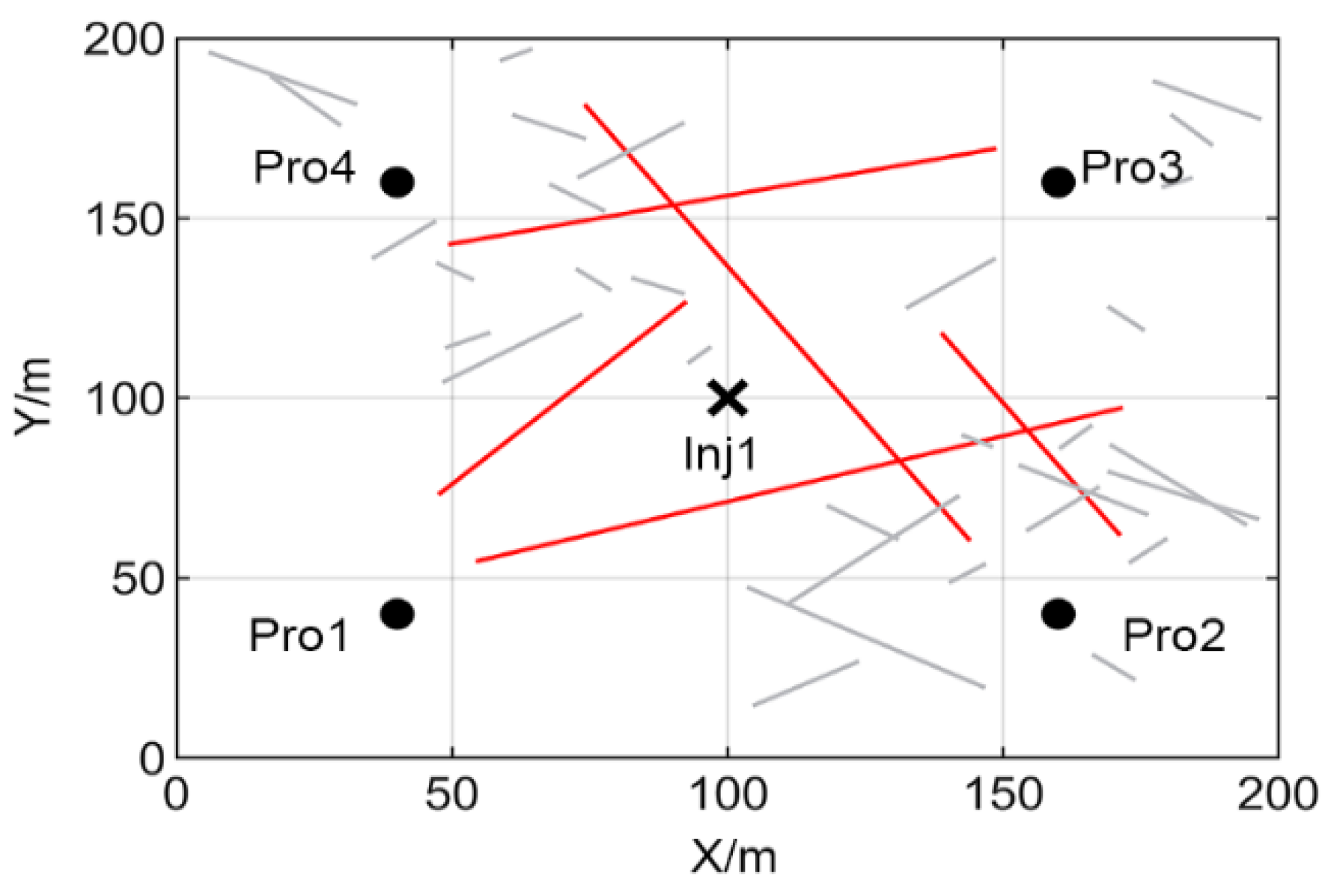
3.1. Two-Dimensional Fractured Reservoir Model

As shown in Figure 6, a synthetic naturally fractured reservoir is defined as a 200 m × 200 m region and divided into 50 × 50 grids. The fracture network, generated by using the multi-scale parameterization method, contains five major fractures (red lines) and two sets of minor fractures (gray lines).

Table 2. Initial range and true value of major fractures for the 2D case.

	x-Coordinate (m)		y-Coordinate (m)		Length (m)		Orientation (Degrees)
Fracture	True	Initial Range	True	Initial Range	True	Initial Range	True	Initial Range
1	109	90–130	121	100–140	140	130–150	120	80–130
2	113	90–130	76	70–100	125	100–130	20	10–40
3	99	80–120	156	120–160	103	90–120	15	10–50
4	70	60–100	100	80–130	70	60- 80	50	30–80
5	155	130–160	90	70–120	65	50–70	120	100–150

and

Table 3. Initial range and true value of small-scale fracture parameters for the 2D case.

Parameters	True Value	Initial Range
Fractal Dimension	1.6	1.4–1.7
Intensity D1 (Set 1)	0.45	0.3–0.6
Intensity D2 (Set 2)	1−D1	-
Mean of Orientation (Set 1)	35	45–75
Sd of Orientation (Set 1)	10	8–15
Mean of Orientation (Set 2)	150	138–178
Sd of Orientation (Set 2)	10	8–15
Proportion Score of Region 1	0.1	0.1–1
Proportion Score of Region 2	0.3	0.1–1
Proportion Score of Region 3	0.1	0.1–1
Proportion Score of Region 4	0.3	0.1–1

present the reference values and prior range used to generate the major and minor fractures. The permeability and porosity of the matrix are set as 3 md and 0.25, respectively. The fracture porosity is set as 0.2, and the cubic law is used to model the permeability of fractures. There is one water injector and four producers; the bottom hole pressure for the producers is set to 100 bars, and the water injection rate for the injectors is set to 30 m³/day. The 900 day historical data of the well oil production rate (WOPR) and the well water production rate (WWPR) are obtained by adding Gaussian noise to the numerical simulation data. The mean value and standard deviation of the noise are set to 0 and 5% of the simulated data. During the simulation, the interval of each time-step is set as 30 days. Therefore, the historical observation data have 30 time-steps and 8 features (OPR and WPR of four producers).

Then, we generate 2000 prior realizations of the fracture network and perform EDFM numerical simulation to obtain corresponding production data as the data set. The data set is divided into a training set, a validation set, and a test set according to the ratio of 0.8:0.1:0.1 (1600:200:200). The validation set is used to adjust the hyperparameters of the surrogate model, and the resulting model structure is shown in Table 1. Figure 7 shows three prior realizations of fracture network and its production data of the Pro1 well. It can be seen that with the change in the fracture distribution, the production dynamics are also significantly different. This is consistent with the understanding that fracture distribution is the main influencing factors of fluid flow in naturally fractured reservoirs. In the following experiments, we investigate the ability of the proposed surrogate to model the mapping relationship between these fracture distributions and production dynamics.

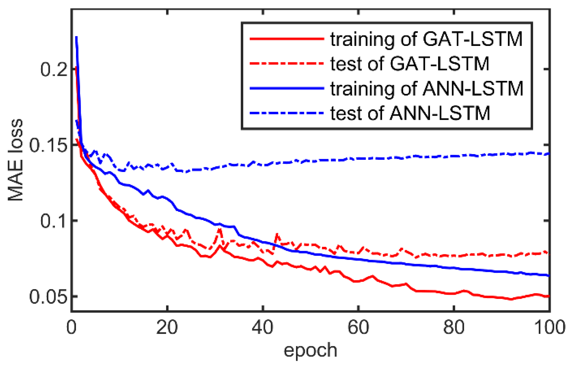
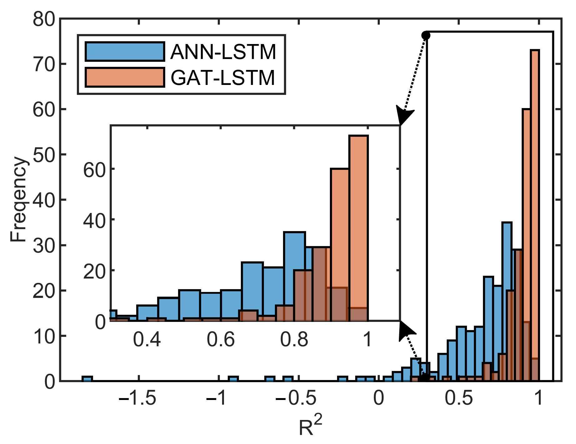
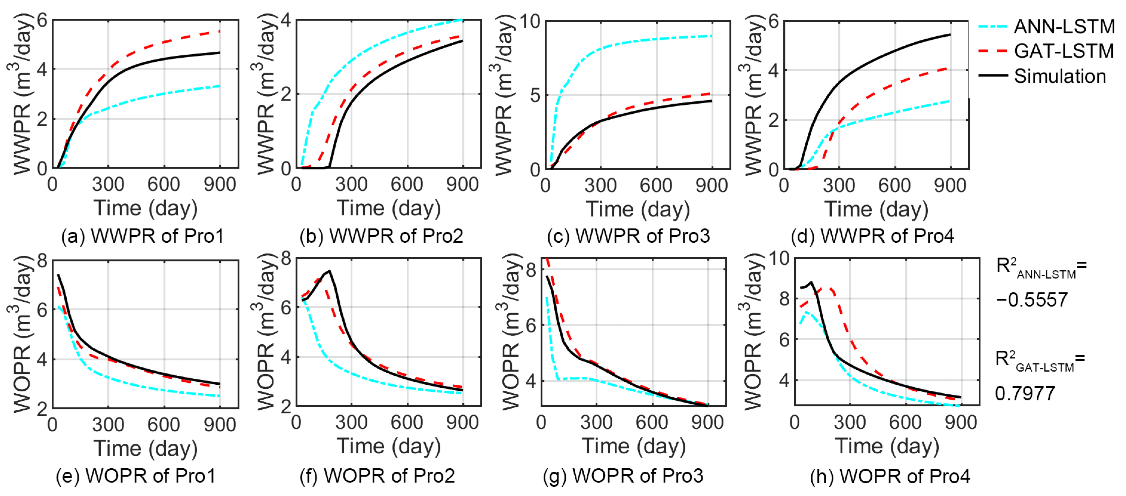
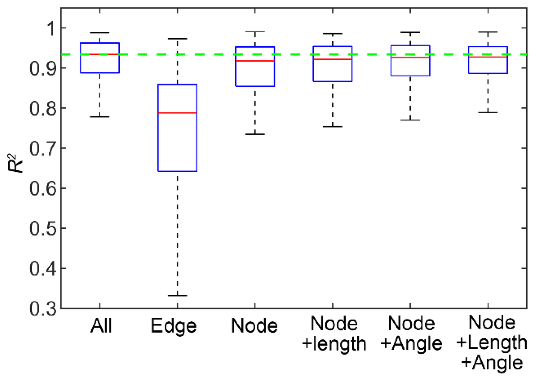
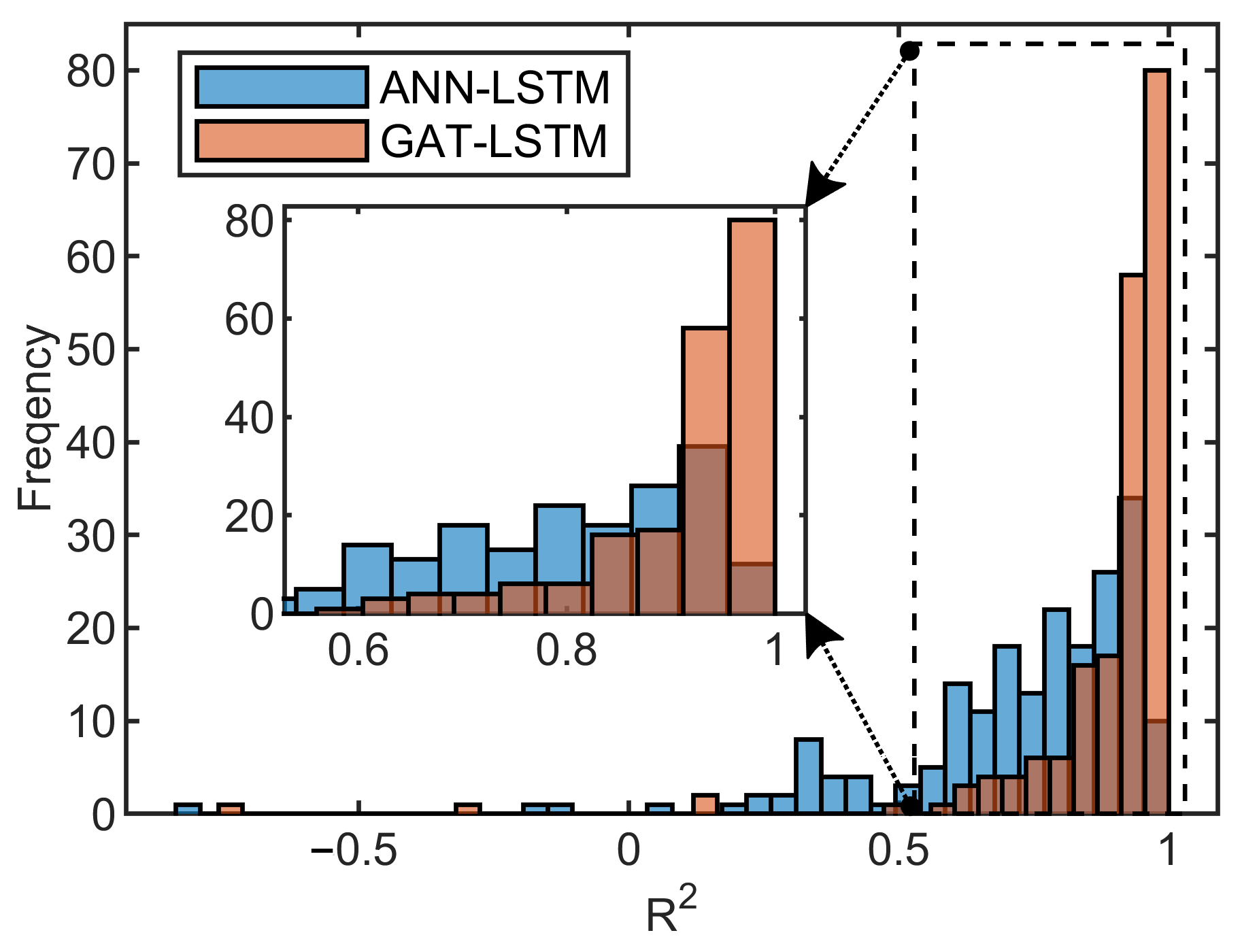
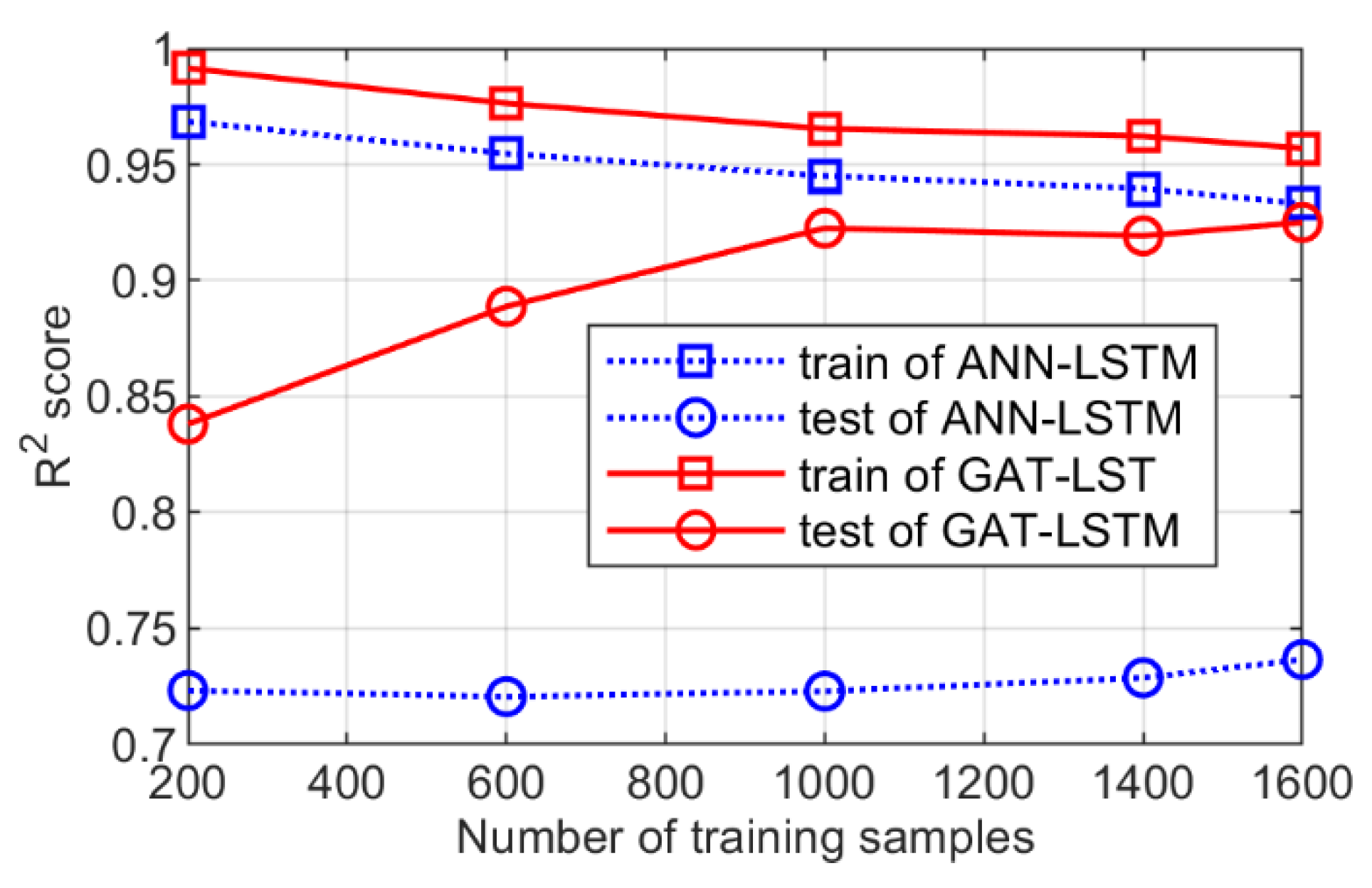
3.2. Analysis of the Surrogate Model Performance

In order to illustrate the performance of the surrogate model with respect to the size of training samples, we used five groups of training samples of different sizes and repeated training for each group of samples three times to obtain the average R² score on the training set and test set, as shown in Figure 8. It can be seen that the R² of the ANN-LSTM model on the training set and the test set is very different, and the R² on the test set does not improve significantly with the increase of the training sample. This indicates that the fracture network features cannot be extracted effectively by using the ANN. In contrast, the R² of the GAT-LSTM model on the test set has significantly improved with the increase of training samples, with the average R² of 0.8380 and 0.9225 using 200 and 1000 training samples, respectively. In addition, we see that after the number of training samples reaches 1000, the R² of the GAT-LSTM model on the test set change smoothly. These results demonstrate that the GAT model can extract the fracture network features effectively and the GAT-LSTM model exhibits preferable generalization performance. In this experiment, both the ANN and GAT learn from identical fracture network parameters. In the ANN model, all fractures feature within a network are collectively transformed, whereas in the GAT model, the transformation of each fracture feature remains independent, aligning with the discrete characteristics inherent in the fracture network. Hence, the comparison of prediction results using the ANN and GAT models reveals that retaining the fracture structure information and discrete characteristics enhances the efficacy of learning features in fracture networks.

Moreover, for a more detailed comparison, the ANN-LSTM and GAT-LSTM models, trained with 1600 samples, are employed in the following experiments. Figure 9 presents the change in the MAE loss function of the GAT-LSTM and ANN-LSTM models during the training process. It can be seen that the ANN-LSTM model is overfitting, and the loss function on the test set continues to rise after 20 epochs. For the GAT-LSTM model, the loss function converges smoothly after 80 epochs. Then, we analyze the prediction performance of the ANN-LSTM and GAT-LSTM models on the test set. Figure 10 shows the R² distribution histograms of the ANN-LSTM model and the GAT-LSTM model across 200 test samples. It can be seen that the R² value of the ANN-LSTM model is negative for certain samples, and the R² value of many test samples is below 0.8. In contrast, the GAT-LSTM model shows a concentration of R² values between 0.8 and 1 for the test samples.

Table 4. The ratio of R² greater than 0.8, 0.9, and 0.95 in the validation set.

Surrogate Model	R2 > 0.8	R2 > 0.85	R2 > 0.9
ANN-LSTM	33%	15.5%	6%
GAT-LSTM	91%	81%	66.5%

summarizes the proportion of test samples in the validation set with R² values exceeding 0.8, 0.9, and 0.95, respectively. It can be seen that the prediction performance of the GAT-LSTM model is significantly better than that of the ANN-LSTM model.

Figure 11 depicts the predicted results of production data for a selected test sample with a negative R² predicted by the ANN-LSTM model. As observed in Figure 10, the negative R² of ANN-LSTM is attributed to its oil production predictions for producer Pro2, which deviate from the trend of numerical simulation results. In the initial 300 days, the WOPR of the numerical simulation rises and falls, whereas the WOPR predicted by ANN-LSTM continues to decline. On the contrary, the GAT-LSTM model can predict the production dynamics more accurately. Particularly for Pro2 and Pro3, the trends of WOPR can be accurately predicted, although there is a large error in the production prediction of Pro4.

Then, the test sample corresponding to P50 of R² value of GAT-LSTM is selected to compare the predicted production data with the numerical simulation results, as shown in Figure 12. It is evident that the GAT-LSTM model can accurately predict the production dynamics overall, aligning well with numerical simulation results. Particularly, it exhibits precision in prediction of WOPR. However, there are errors in the prediction results for water yield, attributed to the complexity introduced by the existence of fractures in the waterflooding process. Future efforts should concentrate on enhancing the predictive accuracy of water production.

Afterward, we evaluate the sensitivity of the GAT-LSTM model to input data variability. To keep the model structure unchanged, we designate the input parameters to be masked with a value of 0. In this comparison, 1000 training samples were used. As shown in Figure 13, we test the model performance with different combination of input data. Taking the model performance obtained using all input parameters (All) as a reference (dotted green line), it can be seen that the model trained using only edge features (Edge) and ignoring the position features of the nodes cannot make the effective prediction. On the contrary, better model performance can be obtained by using only the location features of fractures (Node). This shows that the location of fracture is the key feature of the fracture network. This is due to the location of fractures determining the spatial distribution pattern of the fracture network. In addition, it can be seen that adding the length or angle features to the node features can enhance the prediction performance of the model. In this case, the aperture and permeability of fracture are proportional to the length, so no independent testing was performed. The comparison results show that the prediction performance of the model using all features is the best.

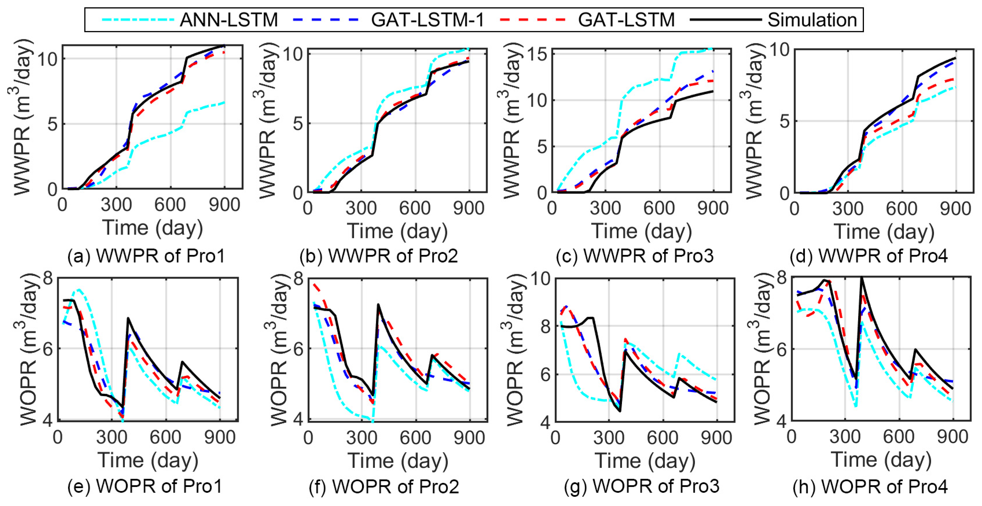
3.3. Test the Performance of the Model under Varying Operational Conditions

Furthermore, we test the prediction performance of the surrogate model under varying operational conditions. Maintain the existing configurations of the 2D reservoir case and only change the injection strategy for the injection well. The injection rate is set as 30 m³/day from days 0 to 330, 40 m³/day from days 330 to 630, and 60 m³/day from days 630 to 900. For this test, 1200 samples were generated, of which 1000 samples were used for training the model and 200 samples were used for testing. The structure of the surrogate model and the training strategy remain unchanged. Figure 14 shows the change in the loss function during training process.

Figure 15 presents the distribution histogram of the prediction performance metrics R² of the GAT-LSTM and ANN-LSTM model for the test samples. It can be seen that the GAT-LSTM model obtains a good prediction performance, 71.5% of test samples with R² greater than 0.9, and the P50 of R² reached 0.9422. On the contrary, the R² of the ANN-LSTM model is dispersed, the samples with R² greater than 0.9 only account for 24.5%, and the P50 of R² is 0.7959. Figure 16 shows the production prediction results of the test sample corresponding to P50 of R² value of the GAT-LSTM model. It can be seen that the GAT-LSTM model has a good consistency with the numerical simulation results, while the ANN-LSTM model has a large prediction bias. In addition, it can be seen that both the GAT-LSTM model and the ANN-LSTM model can capture the changes in production dynamics on day 330 and day 630. This is due to the use of the multi-layer recurrent neural network. For comparison, we use one LSTM layer to obtain the GAT-LSTM-1 model, keeping other hyperparameters unchanged. It can be seen that the overall prediction effect of GAT-LSTM-1 is close to that of the GAT-LSTM model, but it fails to capture the change om production dynamics on day 630.

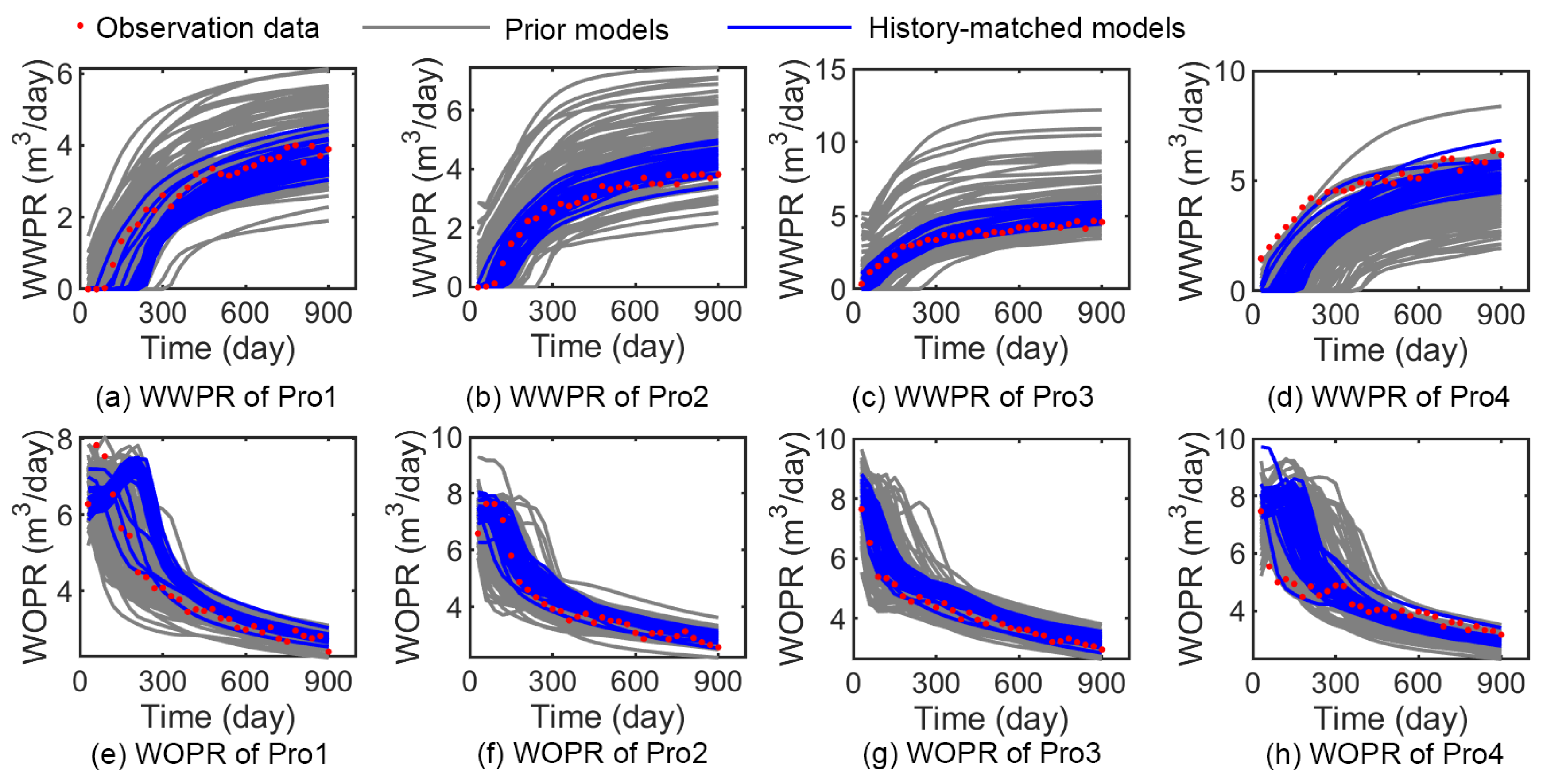
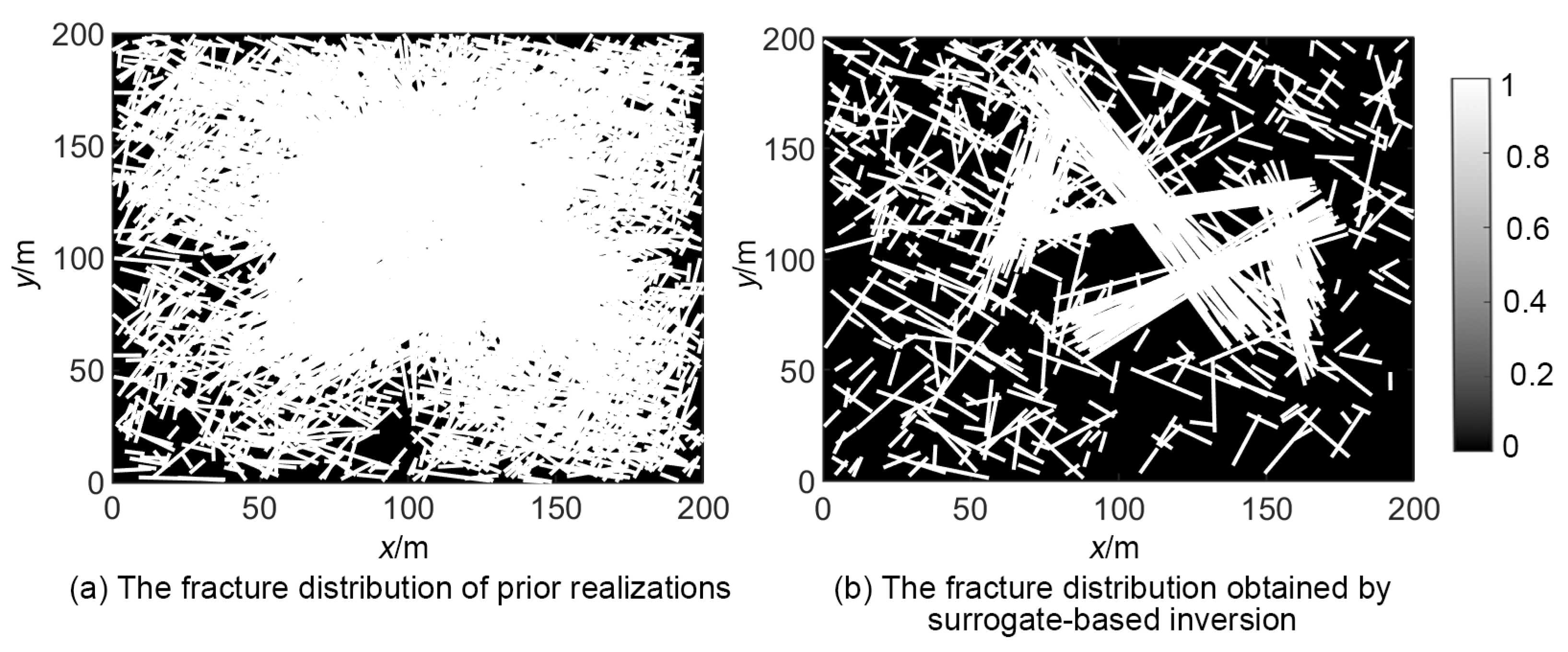
3.4. Results of Surrogate-Based Inverse Modeling

Afterward, we conducted inverse modeling utilizing the GAT-LSTM model. In this experiment, the population size and the number of iterations for the DE algorithm were configured as 100 and 200, respectively. Employing a large population size is beneficial for preserving diversity within the optimization process. This setup entails a total of 20,000 function evaluations. The values of mutation factor F and crossover probability CR of the DE algorithm were set to 0.5 and 0.5, respectively. Figure 17 shows the change process of the objective function during the solution process of the history matching problem utilizing the trained GAT-LSTM surrogate model. It can be seen that the history matching objective function continues to decline with the surrogate-based optimization process and gradually converges after 145 iterations. After the surrogate-based inverse modeling, we use numerical simulation to verify the obtained solutions and 31 solutions with good fitting results are selected. As depicted in Figure 18, the gray curves represent the production data corresponding to 100 prior realizations, the blue curves represent the production data corresponding to the 31 history-matched models, and the red dot signifies the observation data. It can be observed that, in comparison with prior realizations, the discrepancy between the production data and the observed data of history-matched models is significantly reduced.

Finally, Figure 19 compares the fracture distribution probability plot of prior realizations with that of the history-matched models. It can be seen that the fractures of prior realizations (Figure 19a) are distributed throughout the reservoir region due to the large prior range of the uncertainty parameters. After the surrogate-based inverse modeling, the distribution of major fractures is corrected (Figure 19b), and four of the major fracture distributions are accurately predicted, but the predicted results of one major fracture distributions between well Pro3 and Pro4 are significantly different from the true model. This is due to the multiple solutions of history matching. By this comparison, it can be seen that the uncertainty of fracture distribution decreases significantly after inverse modeling.

The results above demonstrate the effectiveness of the proposed GAT-LSTM surrogate model in the application of inverse modeling for naturally fractured reservoirs. In this study, we did not perform the comparison between surrogate-based inverse modeling and simulation-based inverse modeling. The 20,000 evaluations of the history matching objective function based on the EDFM numerical simulation are time-consuming, taking about 1~2 min per simulation for the 2D fractured reservoir model, and even tens of minutes in some cases due to convergence difficulties. As shown in

Table 5. Comparison of computation time between surrogate-based and simulation-based inversion methods, the unit of time is minutes.

Inversion Method	Building the Data Set	Training the Model	DE Optimization	Evaluation of the Solutions	Total Time
Surrogate-based	150	2	10	10	172
Simulation Based	-	-	2000	-	2000

, we compare the computation times between the surrogate- and simulation-based inversion modeling methods. As depicted in Figure 7, it can be observed that only 1000 to 1500 numerical simulations are needed to train the surrogate model, achieving acceptable prediction performance. Therefore, we use the dataset with 1500 samples for comparison. For this 2D reservoir case, building a dataset with 1500 samples takes about 150 min to run the simulations in parallel on a 16-core Intel i9-12900 processor. Training the surrogate model takes about 2 min, the surrogate-based DE optimization takes about 10 min, and the evaluation of obtained solutions takes about 10 min. The total time of surrogate-based inversion is 172 min. If the simulation-based inversion modeling was performed with the same DE settings, the total runs of simulations required would be 20,000, which takes about 2000 min in the same parallel computing environment. Thus, the overall speedup achieved is over a factor of 10. The timings provided here will vary depending on the optimization algorithm and its configuration, the specifics of the computing device, and the complexity of the reservoir numerical model. In addition, the surrogate model can facilitate the decoupling of numerical simulation and the optimization algorithm in inverse modeling. Numerical simulation is solely utilized for dataset construction and final result evaluation. As a result, large-scale parallel computation can be easily employed and can allow for the termination and regeneration of samples that are difficult to converge in numerical simulation.

4. Conclusions

In this paper, we propose a novel deep graph learning-based surrogate model for inverse modeling of naturally fractured reservoirs with multi-scale fracture network. The proposed GAT-LSTM surrogate model can be trained to predict the production response of a fracture network based on the samples obtained from the 2D EDFM simulation. Firstly, the fracture network is represented as graph data, where the fracture endpoint serves as a graph node, and the coordinates are assigned as node attributes. The fractures themselves constitute the graph edges, with associated properties such as fracture length, orientation, aperture, and permeability serving as edge attributes. Then, the multi-layer GAT block in the GAT-LSTM model is employed to capture the high-level features of the fracture network through three phases: graph embedding, fusion of node and edge features, and aggregation of node features. Subsequently, the extracted features are utilized as inputs for the multi-layer LSTM block to predict the production data. Based on the proposed surrogate model, a surrogate-based inverse modeling workflow was developed for the estimation of fracture distribution, integrating the DE algorithm to optimize the objective function of inversion.

To validate the effectiveness of the proposed surrogate model, numerical experiments were conducted on a 2D naturally fractured reservoir. The results demonstrate that the GAT model can extract the fracture network features effectively and the GAT-LSTM model exhibits preferable generalization performance. The ability of GAT to retain fracture structure information and discrete characteristics enhances the efficacy of learning features in fracture networks. Additionally, the proposed surrogate-based inverse modeling workflow shows promising performance in estimating the fracture distribution. Based on the proposed surrogate-based inverse modeling framework, the estimation of fracture distribution can be quickly realized based on parallel computing facilities, which can promote the real-time management of reservoirs. Although the proposed model shows promising prediction performance in the case studies, we observe that the proposed model has some limitations. Firstly, the GAT-LSTM model is a data-driven model, and effectively collecting data samples to reduce model prediction bias plays an important role in the solution of inverse modeling. Secondly, the current research only focuses on 2D fractured reservoir models, and learning the features of 3D fracture network needs to be further studied. Third, the proposed GAT-LSTM model needs to be further studied in real fractured reservoir cases in future work.

References

1. Abbasi, M.; Sharifi, M.; Kazemi, A. Fluid flow in fractured reservoirs: Estimation of fracture intensity distribution, capillary diffusion coefficient and shape factor from saturation data. J. Hydrol. 2020, 582, 124461. [Google Scholar] [CrossRef]
2. Ghorbanidehno, H.; Kokkinaki, A.; Lee, J.; Darve, E. Recent developments in fast and scalable inverse modeling and data assimilation methods in hydrology. J. Hydrol. 2020, 591, 125266. [Google Scholar] [CrossRef]
3. Tang, M.; Liu, Y.; Durlofsky, L.J. A deep-learning-based surrogate model for data assimilation in dynamic subsurface flow problems. J. Comput. Phys. 2020, 413, 109456. [Google Scholar] [CrossRef]
4. Hamdi, H.; Couckuyt, I.; Sousa, M.C.; Dhaene, T. Gaussian Processes for history-matching: Application to an unconventional gas reservoir. Comput. Geosci. 2017, 21, 267–287. [Google Scholar] [CrossRef]
5. Dachanuwattana, S.; Yu, W.; Sepehrnoori, K. An efficient MCMC history matching workflow using fit-for-purpose proxies applied in unconventional oil reservoirs. J. Pet. Sci. Eng. 2019, 176, 381–395. [Google Scholar] [CrossRef]
6. Zhang, H.; Sheng, J.J. Surrogate-Assisted Multiobjective Optimization of a Hydraulically Fractured Well in a Naturally Fractured Shale Reservoir with Geological Uncertainty. SPE J. 2022, 27, 307–328. [Google Scholar] [CrossRef]
7. Zhang, D.; Li, H. Efficient Surrogate Modeling Based on Improved Vision Transformer Neural Network for History Matching. SPE J. 2023, 28, 3046–3062. [Google Scholar] [CrossRef]
8. Zhong, Z.; Sun, A.Y.; Ren, B.; Wang, Y. A Deep-Learning-Based Approach for Reservoir Production Forecast under Uncertainty. SPE J. 2021, 26, 1314–1340. [Google Scholar] [CrossRef]
9. Zhang, K.; Zhang, J.; Ma, X.; Yao, C.; Zhang, L.; Yang, Y.; Wang, J.; Yao, J.; Zhao, H. History Matching of Naturally Fractured Reservoirs Using a Deep Sparse Autoencoder. SPE J. 2021, 26, 1700–1721. [Google Scholar] [CrossRef]
10. Chen, G.; Luo, X.; Jiao, J.J.; Jiang, C. Fracture network characterization with deep generative model based stochastic inversion. Energy 2023, 273, 127302. [Google Scholar] [CrossRef]
11. Yan, B.; Xu, Z.; Gudala, M.; Tariq, Z.; Finkbeiner, T. Reservoir Modeling and Optimization Based on Deep Learning with Application to Enhanced Geothermal Systems. In Proceedings of the SPE Reservoir Characterisation and Simulation Conference and Exhibition, Abu Dhabi, United Arab Emirates, 24–26 January 2023. [Google Scholar]
12. Kim, Y.D.; Durlofsky, L.J. Neural network surrogate for flow prediction and robust optimization in fractured reservoir systems. Fuel 2023, 351, 128756. [Google Scholar] [CrossRef]
13. Rao, X. A generic workflow of projection-based embedded discrete fracture model for flow simulation in porous media. Comput. Geosci. 2023, 27, 561–590. [Google Scholar] [CrossRef]
14. Xu, Y.; Sepehrnoori, K. Modeling fracture transient flow using the Embedded Discrete Fracture Model with nested local grid refinement. J. Pet. Sci. Eng. 2022, 218, 110882. [Google Scholar] [CrossRef]
15. Shaked, B.; Uri, A.; Eran, Y. How Attentive are Graph Attention Networks? In Proceedings of the International Conference on Learning Representations, Virtual Event, 25–29 April 2022.
16. Veličković, P.; Cucurull, G.; Casanova, A.; Romero, A.; Liò, P.; Youshua, B. Graph Attention Networks. In Proceedings of the 6th International Conference on Learning Representations, Toulon, France, 24–26 April 2017. [Google Scholar]
17. Hochreiter, S.; Schmidhuber, J. Long Short-Term Memory. Neural Comput. 1997, 9, 1735–1780. [Google Scholar] [CrossRef] [PubMed]
18. Yang, S.; Yu, X.; Zhou, Y. Lstm and gru neural network performance comparison study: Taking yelp review dataset as an example. In Proceedings of the 2020 International Workshop on Electronic Communication and Artificial Intelligence (IWECAI), Shanghai, China, 12–14 June 2020; pp. 98–101. [Google Scholar]
19. Wang, N.; Chang, H.; Kong, X.-Z.; Zhang, D. Deep learning based closed-loop well control optimization of geothermal reservoir with uncertain permeability. Renew. Energy 2023, 211, 379–394. [Google Scholar] [CrossRef]
20. Bhatti, U.A.; Tang, H.; Wu, G.; Marjan, S.; Hussain, A. Deep learning with graph convolutional networks: An overview and latest applications in computational intelligence. Int. J. Intell. Syst. 2023, 2023, 8342104. [Google Scholar] [CrossRef]
21. Chen, Y.; Wu, L.; Zaki, M. Iterative deep graph learning for graph neural networks: Better and robust node embeddings. Adv. Neural Inf. Process. Syst. 2020, 33, 19314–19326. [Google Scholar]
22. Xia, F.; Sun, K.; Yu, S.; Aziz, A.; Wan, L.; Pan, S.; Liu, H. Graph learning: A survey. IEEE Trans. Artif. Intell. 2021, 2, 109–127. [Google Scholar] [CrossRef]
23. Mohamed, H.A.; Pilutti, D.; James, S.; Del Bue, A.; Pelillo, M.; Vascon, S. Locality-aware subgraphs for inductive link prediction in knowledge graphs. Pattern Recognit. Lett. 2023, 167, 90–97. [Google Scholar] [CrossRef]
24. Ling, C.; Jiang, J.; Wang, J.; Thai, M.T.; Xue, R.; Song, J.; Qiu, M.; Zhao, L. Deep graph representation learning and optimization for influence maximization. In Proceedings of the International Conference on Machine Learning, Sanya, China, 27–29 December 2023; pp. 21350–21361. [Google Scholar]
25. Gligorijević, V.; Renfrew, P.D.; Kosciolek, T.; Leman, J.K.; Berenberg, D.; Vatanen, T.; Chandler, C.; Taylor, B.C.; Fisk, I.M.; Vlamakis, H. Structure-based protein function prediction using graph convolutional networks. Nat. Commun. 2021, 12, 3168. [Google Scholar] [CrossRef]
26. Ma, X.; Zhang, K.; Yao, C.; Zhang, L.; Wang, J.; Yang, Y.; Yao, J. Multiscale-Network Structure Inversion of Fractured Media Based on a Hierarchical-Parameterization and Data-Driven Evolutionary-Optimization Method. SPE J. 2020, 25, 2729–2748. [Google Scholar] [CrossRef]
27. Aghli, G.; Moussavi-Harami, R.; Mohammadian, R. Reservoir heterogeneity and fracture parameter determination using electrical image logs and petrophysical data (a case study, carbonate Asmari Formation, Zagros Basin, SW Iran). Pet. Sci. 2020, 17, 51–69. [Google Scholar] [CrossRef]
28. Klimczak, C.; Schultz, R.; Parashar, R.; Reeves, D. Cubic law with aperture-length correlation: Implications for network scale fluid flow. Hydrogeol. J. 2010, 18, 851–862. [Google Scholar] [CrossRef]
29. Xu, J.; Li, Z.; Du, B.; Zhang, M.; Liu, J. Reluplex made more practical: Leaky ReLU. In Proceedings of the 2020 IEEE Symposium on Computers and Communications (ISCC), Rennes, France, 7–10 July 2020; pp. 1–7. [Google Scholar]
30. Ma, X.; Zhang, K.; Zhao, H.; Zhang, L.; Wang, J.; Zhang, H.; Liu, P.; Yan, X.; Yang, Y. A vector-to-sequence based multilayer recurrent network surrogate model for history matching of large-scale reservoir. J. Pet. Sci. Eng. 2022, 214, 110548. [Google Scholar] [CrossRef]
31. Bao, K.; Lie, K.-A.; Møyner, O.; Liu, M. Fully implicit simulation of polymer flooding with MRST. Comput. Geosci. 2017, 21, 1219–1244. [Google Scholar] [CrossRef]
32. Shah, S.; Møyner, O.; Tene, M.; Lie, K.-A.; Hajibeygi, H. The multiscale restriction smoothed basis method for fractured porous media (F-MsRSB). J. Comput. Phys. 2016, 318, 36–57. [Google Scholar] [CrossRef]
33. Storn, R.; Price, K. Differential Evolution—A Simple and Efficient Heuristic for global Optimization over Continuous Spaces. J. Glob. Optim. 1997, 11, 341–359. [Google Scholar] [CrossRef]
34. Abadi, M.; Agarwal, A.; Barham, P.; Eugene, B. TensorFlow: Large-Scale Machine Learning on Heterogeneous Distributed Systems. arXiv 2016, arXiv:1603.04467. [Google Scholar]
35. Ferludin, O.; Eigenwillig, A.; Blais, M.; Zelle, D.; Pfeifer, J.; Sanchez-Gonzalez, A.; Li, W.L.S.; Abu-El-Haija, S.; Battaglia, P.; Bulut, N. Tf-gnn: Graph neural networks in tensorflow. arXiv 2022, arXiv:2207.03522. [Google Scholar]
36. Kingma, D.P.; Ba, J. Adam: A Method for Stochastic Optimization. arXiv 2014, arXiv:1412.6980. [Google Scholar]
Figure 1. The schematic diagram of a fracture and its graph representation.
Mathematics 12 00754 g001
Figure 2. Framework of the proposed GAT-LSTM surrogate model.
Mathematics 12 00754 g002
Figure 3. Illustration of the attention operator by node i on its neighborhood.
Mathematics 12 00754 g003
Figure 4. Flowchart of the proposed GAT-LSTM model.
Mathematics 12 00754 g004
Figure 5. The proposed surrogate-based inverse modeling workflow.
Mathematics 12 00754 g005
Figure 6. The reference model with major (red lines) and minor (gray lines) fractures.
Mathematics 12 00754 g006
Figure 7. Three prior realization of the fracture network and their corresponding production data. In (ac), the red lines represent large-scale fractures and the gray lines represent small-scale fractures.
Mathematics 12 00754 g007
Figure 8. The relationship between the R2 and the size of training samples.
Mathematics 12 00754 g008
Figure 9. The evolution of the loss function during the training process of the GAT-LSTM and ANN-LSTM models.
Mathematics 12 00754 g009
Figure 10. Comparison of R2 score distribution histograms between the ANN-LSTM model and the GAT-LSTM model.
Mathematics 12 00754 g010
Figure 11. The predicted results of production data for the test sample with a negative R2 predicted by the ANN-LSTM model.
Mathematics 12 00754 g011
Figure 12. Comparison of well rates from the numerical simulator and surrogate model for the P50-R2 test samples of GAT-LSTM model.
Mathematics 12 00754 g012
Figure 13. The sensitivity of the GAT-LSTM model to input data variability. The dotted green line is the median value of R2 obtained using all input parameters.
Mathematics 12 00754 g013
Figure 14. The evolution of the loss function during the training process of the GAT-LSTM and ANN-LSTM models under varying operational conditions.
Mathematics 12 00754 g014
Figure 15. Comparison of R2 score distribution histograms between the ANN-LSTM model and GAT-LSTM model under varying operational conditions.
Mathematics 12 00754 g015
Figure 16. Comparison of well rates prediction under varying operational conditions for the P50 test samples of GAT-LSTM model.
Mathematics 12 00754 g016
Figure 17. The optimization process of surrogate-based inverse modeling.
Mathematics 12 00754 g017
Figure 18. The matching results of the observation data.
Mathematics 12 00754 g018
Figure 19. The inversion results of the fracture distribution.
Mathematics 12 00754 g019