The Ruler Sequence Revisited: A Dynamic Perspective

Abstract

The Ruler function or the Gros sequence is a classical infinite integer sequence that underlies some interesting mathematical problems. In this paper, we provide four new problems containing this type of sequence: (i) demographic discrete dynamical automaton, (ii) the middle interval Cantor set, (iii) construction by duplication of polygons and (iv) the horizontal visibility sequence at the accumulation point of the Feigenbaum cascade. In all of them, the infinite sequence is obtained through a recursive procedure of duplication. The properties of the ruler sequence, in particular, those relating to recursiveness and self-containing, are used to achieve a deeper understanding of these four problems. These new representations of the ruler sequence could inspire new studies in the field of discrete mathematics.

1. Introduction

The Ruler sequence, also known as the ruler function, is referenced in the OEIS (On-Line Encyclopedia of Integer Sequences), specifically in Sequence A001511 [1], where various definitions are presented. This infinite integer sequence is commonly defined by its nth term, which represents the highest power of 2 that divides $2n$, for $n=1,2,\dots$. It is also termed the Gros sequence by Hinz et al. [2], who tackled the so-called Baguenaudier or Chinese Ring Puzzle problem (involving the disentanglement of rings linked together in a wire) and obtained the first terms of the ruler sequence as a finite solution.

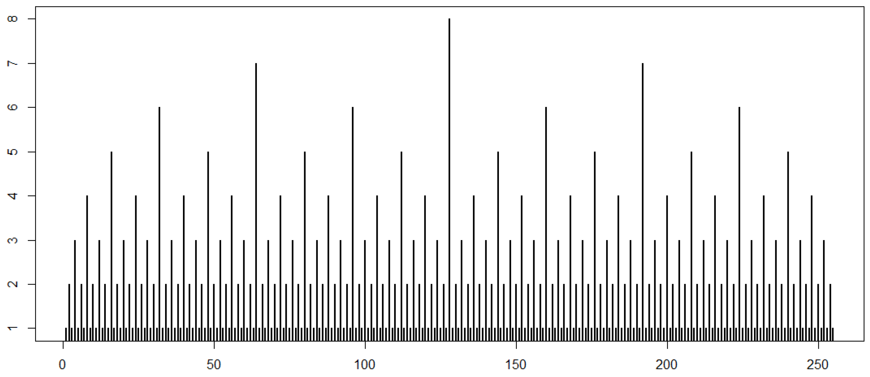
The initial terms of this sequence are given by $1,2,1,3,1,2,1,4,1,2,1,3,1,2,1,\dots$, and the first $2^8-1$ terms are visualized in Figure 1, resembling the ticks on a ruler. In this paper, we explore four additional problems in discrete mathematics where this sequence emerges as a characteristic of their recursive nature: (i) demographic automaton, (ii) the middle interval Cantor set, (iii) construction by duplication of polygons, and (iv) the horizontal visibility of the Feigenbaum cascade.

Many significant sequences arise as solutions to discrete dynamical models [3], where the sequence represents the variable’s value (e.g., population size) at each time step. The sequence forms the trajectory of the initial value problem, extending theoretically to an infinite number of time steps, given an initial condition. Perhaps one of the earliest historical examples of such a discrete model is the one leading to the Fibonacci sequence [4], where the nth term is the sum of the two preceding terms: $X\left(n\right)=X(n-1)+X(n-2)$ for $n>2$, with initial conditions $X\left(1\right)=X\left(2\right)=1$. In contrast to this simple model, many population models incorporate spatial variables and individuals’ ages [5]. Cellular automata [6] provide a specific approach to handling such spatial demographic models.

Sharing equal significance with these discrete dynamical systems is the Cantor set, a cornerstone in number theory, combinatorics, and fractal theory [7,8]. It is often asserted that the Cantor set encapsulates essential elements of these mathematical disciplines [9]. Originating from the unit interval, the classical ternary Cantor set is recursively formed by dividing the resulting intervals into three subintervals, omitting the central one at each step. This process gives rise to one of the most renowned fractal sets.

Polygons, defined as planar figures bounded by three or more sides, are among the most extensively studied geometric shapes [10]. A polygon with s vertices or sides is referred to as an s-gon. The construction of polygons is a longstanding problem [11,12], and the manipulation of polygons is a popular subject in geometry [13]. Various problems aim to explore the properties of polygons and establish connections with other geometric figures. For instance, “chopping polygons into triangles” and related issues, such as frieze patterns, reveal collective properties emerging from simple local rules [13]. The duplication of sides of polygons inscribed within a unit radius circle can be employed to estimate the value of $\pi$ [11]. This procedure is applicable to regular polygons, i.e., those with all sides and angles equal, but it is not a strict requirement.

A logistic map exhibits chaotic behavior for specific values of growth rate. In the classical model $x_{n+1}=r{x}_n(1-x_n)$, chaos emerges and disappears infinitely as the growth rate r increases from 1 to 4, following well-studied bifurcations [8,14,15]. The bifurcation diagram has been reinterpreted by applying the horizontal visibility algorithm [16], obtaining special types of graphs denominated Feigenbaum graphs [17]. Recently, new patterns in sequences derived from the horizontal visibility algorithm within the infinite cascades leading to chaos in this bifurcation diagram have been uncovered [18].

Common to all four problems is their capacity to generate the ruler or Gros sequence, acting as a distinctive fingerprint of their properties. In the following section, we provide a brief overview of the ruler function and its properties. Section three introduces an alternative procedure for obtaining the ruler sequence through duplication. The subsequent sections then apply this procedure to the four problems, where the ruler sequence is inherent. Finally, in Section 8, we present some concluding remarks.

2. Some Classical Descriptions of the Ruler Function

As highlighted in the introduction, the ruler sequence is recognized for its connection to classical problems such as the division of even numbers by powers of 2 or the Tower of Hanoi [2]. In the context of the first problem, the ruler sequence $a\left(n\right)$ corresponds to the p-adic valuation of $2n$. In the case of the Tower of Hanoi, the ruler sequence aligns with the sequence of movements required for its solution; if we enumerate the discs on one of the three pegs in ascending order of diameter and encode the movements between pegs at each step, the resulting sequence coincides with the ruler sequence [2]. According to [2], this sequence can be recursively described by the function g:

$$g_k=\{\begin{array}{cccc}1\hfill & \mathrm{if}& k\hfill & \mathrm{odd}\hfill \\ g_{k/2}+1\hfill & \mathrm{if}& k\hfill & \mathrm{even}\hfill \end{array}$$

(1)

Another characterization of the ruler sequence, reflecting the corresponding property of the Gray code (numerical code in which consecutive integers are represented by binary numbers differing by only one digit), is given by [2]:

$$\begin{array}{ccccc}{g}_{2^n}\hfill & =& n+1\hfill & \mathrm{if}& n\in {\mathbb{N}}_0\hfill \\ g_{2^n+k}\hfill & =& g_{2^n-k}\hfill & \mathrm{if}& k\in [2^n-1]\hfill \end{array}$$

(2)

A straightforward and practical method for generating a ruler sequence of size $n_{max}$ is demonstrated by the following script [19], implemented in R [20]:

• nmax = 8;
• r = 1;
• for (n in 2:nmax){
•  r =c(r,n,r)
•  }

Figure 1 is generated using this algorithm, with $n_{max}=8$.

Some authors consider the ruler sequence and Thomae’s function to be synonymous (see, for instance, [21]). In fact, the ruler sequence can be seen as a restriction of Thomae’s function to the dyadic rationals—those rational numbers whose denominators are powers of 2. If we define

$$h\left(x\right)=\{\begin{array}{cc}{2}^{-k}& \mathrm{if}x=\frac{p}{2^k}\mathrm{with}p\mathrm{odd}\hfill \\ 0& \mathrm{otherwise}\hfill \end{array}$$

(3)

the ruler sequence coincides, after a linear translation, with the sequence of the exponents of the image of the set of dyadic rationals by h, ordered from least to greatest. For instance, if we restrict the dyadic rationals to those that have a power n of less than 4, the ordered image of h is

$$\frac{1}{2^4},\frac{1}{2^3},\frac{1}{2^4},\frac{1}{2^2},\frac{1}{2^4},\frac{1}{2^3},\frac{1}{2^4},\frac{1}{2},\frac{1}{2^4},\frac{1}{2^3},\frac{1}{2^4},\frac{1}{2^2},\frac{1}{2^4},\frac{1}{2^3},\frac{1}{2^4}$$

(4)

whose sequence of exponents is

$$-4,-3,-4,-2,-4,-3,-4,-1,-4,-3,-4,-2,-4,-3,-4$$

This sequence can be moved to yield positive integers by adding the largest absolute number plus 1, in this case, $4+1=5$, to all the members of the sequence:

$$1,2,1,3,1,2,1,4,1,2,1,3,1,2,1$$

The same transformation can be carried out for any n, and hence, we can obtain the infinite ruler sequence.

As mentioned in the Introduction, alternative descriptions of the ruler function can be found in [1]. This section concludes by highlighting some specific properties of the ruler sequence: it is self-containing, meaning it contains a proper subsequence that is identical to itself, and it is regular [22] and square-free [23]. However, according to Kimberling’s definition, it is not considered a fractal sequence [22]. Notably, this sequence verifies that after deleting the first occurrence of each positive integer, the remaining sequence is the same as the original. These attributes will become even more evident as we delve into the recursive definition and explore the problems presented in the following sections.

3. An Alternative Derivation of the Ruler Sequence

Let us consider a sequence of successive partitions of an interval $I\in \mathbb{R}$, finite or infinite, obtained via duplication of exclusively the points included in the previous step (see Figure 2). If $x_{n,k}$ is the kth point of the partition appearing in step n, it gives rise to two new points in the next step $n+1$ that satisfy

$$x_{n+1,i}<x_{n,k}<x_{n+1,j}$$

(5)

In addition, both $x_{n+1,i}$ and $x_{n+1,j}$ must not overlap with the points inserted in the partition by duplicating other points, i.e., $x_{n+1,i-1}<x_{n+1,i}$ and $x_{n+1,j}<x_{n+1,j+1}$. The other points already present in previous steps, but that do not duplicate, are also added to this next step $n+1$.

The partition of the interval at each step is given by

$$X_n=\{x_{n,1},x_{n-1,1},x_{n,2},\dots ,x_{1,1},\dots ,x_{n,2^{n-1}-1},x_{n-1,2^{n-2}},x_{n,2^{n-1}}\}$$

(6)

For instance, as can be seen in Figure 2,

$$X_1=\left\{x_{11}\right\},X_2=\{x_{2,1},x_{11},x_{2,2}\},X_3=\{x_{3,1},x_{2,1},x_{3,2},x_{1,1},x_{3,3},x_{2,2},x_{3,4}\}$$

(7)

and

$$X_4=\{x_{4,1},x_{3,1},x_{4,2},x_{2,1},x_{4,3},x_{3,2},x_{4,4},x_{1,1},x_{4,5},x_{3,3},x_{4,6},x_{2,2},x_{4,7},x_{3,4},x_{4,8}\}$$

(8)

The schematic representation of the sequence construction depicted in Figure 2 can be viewed as a tree, i.e., a graph without cycles. However, it is important to note that, contrary to classical tree graphs, the nodes on the upper levels are also presented on lower levels with their corresponding indices. These trees share some similarities with the so-called Stern–Brocot trees, which provide positive rational numbers [24].

The sequence of indices at step n, $r_n$, is formed by the index of each point of the partition at this step. Thus, as seen in Figure 2, $r_1=\left\{1\right\}$, $r_2=\{1,2,1\}$ and $r_3=\{1,2,1,3,1,2,1\}$. Once the partition has been updated, we assign the corresponding index to all points of the partition generated in this step as follows: 1 for the newly included points, and an increase of one unit for the rest of points that already belong to the partition. In so doing, the sequence of indices in step n is

$$r_n=\{1,2,1,3,\dots ,n,\dots 3,1,2,1\}$$

(9)

As n tends to infinity, it becomes apparent that this sequence $r_n$ converges to the ruler sequence or Gros sequence [1].

It can be shown that the asymptotic relative frequency of each natural number k in the ruler sequence is $f\left(k\right)=2^{-k}$. Obviously, the sum of these relative frequencies must be 1, i.e.,

$$\sum _k^{\infty }\frac{1}{2^k}=1$$

(10)

Moreover, this relative frequency equals the frequency of any block or motif with a largest natural number k. For instance, the frequency of each of the blocks of size $z=5$ whose largest natural number is $k=5$, i.e.,

$$\begin{array}{ccccc}5& 1& 2& 1& 3\\ 1& 5& 1& 2& 1\\ 2& 1& 5& 1& 2\\ 1& 2& 1& 5& 1\\ 3& 1& 2& 1& 5\end{array}$$

is ${\nu }_5\left(5\right)=2^{-5}$.

This pattern repeats for any digit k of the ruler sequence and for all blocks of size z. When arranging the blocks in such a way that the largest digit is positioned on the main diagonal, the resulting matrix is symmetric. The rows of this matrix contain the ruler sequence up to the term $k-1$ in a circular order, with the first row representing the natural order. Schematically, this can be illustrated as follows:

$$\begin{array}{ccccccc}k& 1& 2& 1& 3& 1& \dots \\ 1& k& 1& 2& 1& 3& \dots \\ 2& 1& k& 1& 2& 1& \dots \\ 1& 2& 1& k& 1& 2& \dots \\ 3& 1& 2& 1& k& 1& \dots \\ 1& 3& 1& 2& 1& k& \dots \\ ⋮& & & & & \end{array}$$

Let us now find the sum of the terms of the index sequence. For instance, $s_1=1$, $s_2=4$, and $s_3=11$. It is not difficult to find a recursive formula for the sequence

$$s_{n+1}=2s_n+n+1$$

(11)

for $n=1,2,\dots$. This expression can be rewritten in terms of $s_1=1$ as

$$s_{n+1}=2^{n-1}+n+1+2n+2^2(n-1)+\dots +2^{n-2}2$$

(12)

for $n=1,2,\dots$.

As the partition is constructed, the size of the successive terms of the index sequence increases. It is straightforward to prove that the number of terms in the sequence in step n is

$$\#r\left(n\right)\equiv N\left(n\right)=2^n-1$$

(13)

which provide exponential growth.

It is also evident that the maximum integer in the nth-term is $max\left(r_n\right)=n$. The ratio between the maximum integer and the length of the nth-term

$$\lambda \left(n\right)=\frac{max\left(r_n\right)}{\#r\left(n\right)}$$

can be expressed as a function of N as

$$\lambda \left(N\right)=\frac{{log}_2(N+1)}{N}$$

4. The Solution of Recursive Demographic Automaton

The process of point generation described in the preceding section draws a parallel with the self-reproduction dynamics within a population. In this analogy, the points generated can be likened to individuals situated in a one-dimensional array. Initially, a singular individual, positioned at a specific spatial location, gives rise to two new individuals placed on each side. Following a rule of duplication, individuals replicate only once, occurring in the subsequent step after their formation. Notably, this model assumes immortality among individuals, signifying the absence of any death rate. Consequently, at each time step, the population in the one-dimensional array undergoes expansion, with the age of individuals at step n denoted by the sequence index $r_n$. Thus, the ruler or Gros sequence serves as a representation of the age distribution within the population situated in the one-dimensional array over infinite time (and infinite space).

The total population at step n, $N\left(n\right)$, follows an exponential growth model, as expressed by Equation (13). This dynamic behavior is derived from the solution of the discrete equation

$$N(n+2)=2\left(N(n+1)-N\left(n\right)\right)+N(n+1)$$

(14)

for $n=1,2,\dots$ and

$$N\left(1\right)=1;N\left(2\right)=2N\left(1\right)+1=3$$

The first term in Equation (14) signifies the duplication of individuals born in the previous step, while the second term accounts for the survival of all individuals from the previous step, each aging by one. Equation (14) can also be written as

$$N(n+2)=3N(n+1)-2N\left(n\right)$$

(15)

taking the form of the so-called Horadam sequences, which include, among others, the Fibonacci and Lucas sequences [25]. This discrete equation provides a mathematical representation of the population dynamics, where the total population at each step is influenced by both the reproduction and aging processes.

It can be easily demonstrated that the difference $N(n+1)-N\left(n\right)=2^n$ for $n=1,2,\dots$, indicating that, at each step n, $2^{n-1}$ individuals in the population have the potential to reproduce, while the remaining population, $2^{n-1}-1$, ages by one unit. This observation highlights the distinct roles played by individuals in the population dynamics: a portion contributes to the expansion of the population through reproduction, while the remainder continues the aging process, maintaining the balance in the overall structure of the population.

It is interesting to note that these equations are equivalent to the discrete equation

$$N(n+1)=2N\left(n\right)+1n=1,2,\dots$$

(16)

with the initial term $N\left(1\right)=1$, which represents the number of movements required to completely move n discs from one peg to another, according to the rules of the Tower of Hanoi game [2].

The age distribution of the population is captured by the expression in Equation (10) and is visualized in the demographic pyramid shown in Figure 3.

The size of the sequences, $r_n$, generated step by step, is a consequence of the spatial arrangement defined in the cellular automaton (refer to, for instance, [26]). As the population growth is unbounded, an array with an infinite number of components is required to represent the evolving sequence over time.

This demographic model can be adapted to account for the mortality of individuals at a specific age. For instance, one might consider dividing an individual’s lifespan into three periods: (i) fertility, (ii) maturity, and (iii) senescence. Under this modification, individuals die and are removed from the population after three time steps. Consequently, the original discrete model in Equation (14) is adjusted to accommodate this mortality effect:

$$r_n=\{\begin{array}{ccc}{2}^n-1& \mathrm{if}\hfill & n=1,2\\ 72^{n-3}& \mathrm{if}\hfill & n=3,4,5,\dots \end{array}$$

(17)

The expression of Equation (17) for $n=3,4,\dots$ is the solution of the geometric equation

$$r_{n+1}=2r_n$$

(18)

This implies that, with this specific death rate, the population duplicates at each step. It is intriguing to note that, even though all individuals eventually succumb to mortality, the population size continues to grow limitlessly. Consequently, to maintain a bounded population, an additional assumption is necessary. This assumption could either reduce the growth rate or accelerate the rate at which individuals disappear. In either scenario, the age distribution is no longer characterized by the ruler sequence.

5. Middle Interval Indices of the Cantor Set

The Cantor set, referenced in [7,8,9], is a fractal subset within the interval $[0,1]$. Geometrically, starting with the unit interval, the classical Cantor set undergoes a process where three equal subintervals of length $l_1=\frac{1}{3}$ are obtained. These subintervals are positioned on each side of the middle open interval: $i_{11}=(\frac{1}{3},\frac{2}{3})$, namely, $[0,\frac{1}{3}]$ and $[\frac{2}{3},1]$. The first term of the sequence of middle intervals is defined as $C_1=i_{11}$ with the index of $i_{11}$ denoted as $r_1=\left\{1\right\}$, indicating the number of steps since $i_{11}$ was formed (see Figure 4).

In the subsequent step, only the first and third intervals are further partitioned into three new subintervals, while the middle interval remains undivided. Consequently, the unit interval is divided into six new subintervals of length $l_2=\frac{1}{9}$, with the previous middle interval now tripling in length: $[0,\frac{1}{9}],(\frac{1}{9},\frac{2}{9}),[\frac{2}{9},\frac{1}{3}],(\frac{1}{3},\frac{2}{3}),[\frac{2}{3},\frac{7}{9}],(\frac{7}{9},\frac{8}{9}),[\frac{8}{9},1]$. The three middle intervals are identified as $i_{21}=(\frac{1}{9},\frac{2}{9})$, $i_{11}=(\frac{1}{3},\frac{2}{3})$, and $i_{22}=(\frac{7}{9},\frac{8}{9})$, with the indices $i_{21}=i_{22}=1$ (indicating their first appearance) and $i_{11}=2$ (existing after 2 steps). The sequence of middle intervals in this step is denoted as $C_2=i_{21},i_{11},i_{22}$, and its corresponding index sequence is $r_2=\{1,2,1\}$.

In the third step, four new middle open intervals emerge: $i_{31}=(\frac{1}{3^3},\frac{2}{3^3})$, $i_{32}=(\frac{7}{3^3},\frac{8}{3^3})$, $i_{33}=(\frac{17}{3^3},\frac{18}{3^3})$, and $i_{34}=(\frac{25}{3^3},\frac{26}{3^3})$. These, along with the previously identified intervals, form the third term of the sequence of middle intervals:

$$C_3=\{i_{31},i_{21},i_{32},i_{11},i_{33},i_{22},i_{34}\}$$

and the associated index sequence:

$$r_3=\{1,2,1,3,1,2,1\}$$

For each step, the nth term of the sequence of middle intervals, $C_n$, contains $2^n-1$ elements (for $n=1,2,\dots$), with the corresponding index sequence $r_n$. A general formula for the nth term of the sequence of intervals is expressed as

$$C_n=\{i_{n1},i_{(n-1)1},i_{n2},i_{(n-2)1},\dots ,i_{11},\dots ,i_{(n-1)2^{(n-2)}},i_{n{2}^{n-1}}\}$$

and the associated index sequence is

$$r_n=\{1,2,1,3,\dots ,n,\dots 3,1,2,1\}$$

It is noteworthy that the construction of the sequences $r_n$ is independent of the way intervals are chosen, relying solely on the number of divisions, which, in this case, is three per step, with a middle interval that remains undivided. As stated in Section 3, the ruler sequence r exclusively emerges through the defined process of subdivision.

The distribution of interval lengths is described by the corresponding index sequence, denoted as $r_n$. For example, considering a case when $n=3$, there are four intervals of length $\frac{1}{3^3}$, two of length $\frac{1}{3^2}$, and one of length $\frac{1}{3}$. Therefore, the total length of the middle intervals forming the nth term of the interval sequence can be expressed as

$$L_n=\sum _k{l}_n{3}^{r_n\left(k\right)-1}$$

(19)

where $l_n$ represents the length of the nth subdivision, i.e., $l_n=3^{-n}$, and the exponent $r_n\left(k\right)$ is interpreted as the kth coordinate of $r_n$. Consequently, this expression can be simplified to

$$L_n=\sum _k{3}^{r_n\left(k\right)-(n+1)}$$

(20)

For instance, the first three whole middle interval lengths are

$$L_1=\frac{1}{3};L_2=\frac{1}{3^2}+\frac{1}{3^1}+\frac{1}{3^2}=\frac{5}{9}$$

(21)

$$L_3=\frac{1}{3^{3+0}}+\frac{1}{3^{3-1}}+\frac{1}{3^{3+0}}+\frac{1}{3^{3-3}}+\frac{1}{3^{3+0}}+\frac{1}{3^{3-1}}+\frac{1}{3^{3-0}}=\frac{19}{27}$$

(22)

This last expression can be also written as

$$L_3=4\frac{1}{3^3}+2\frac{1}{3^2}+\frac{1}{3}$$

(23)

In general, it can be proven that

$$L_n=\sum _{k=1}^n{2}^{k-1}\frac{1}{3^k}=\frac{1}{2}\sum _{k=1}^n{\left(\frac{2}{3}\right)}^k=\frac{1}{2}\left(3\left(1-{\left(\frac{2}{3}\right)}^n\right)-1\right)$$

(24)

This sequence of total lenghts $\left\{L_n\right\}$ tends to 1 as n tends to infinity. Note that this limit coincides with the total length of the complementary of the Cantor set [9].

6. Vertex Indices of Infinite-Sided Polygons

In the introduction, we highlighted the classical problem of constructing polygons with any number of sides, which has yielded fundamental results in both geometry and number theory (see [11,12]). For the sake of simplicity, our focus is on regular s-gons with s vertices, where s is either a prime number, denoted as m, or a power of 2, i.e., $s=2^n$, for $n=1,2,\dots$. 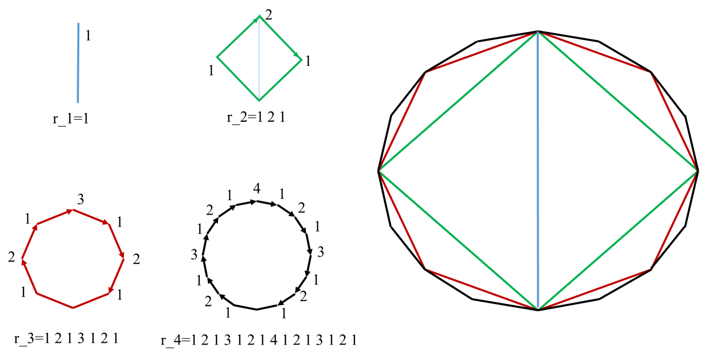As an illustrative example, when each side is equally divided, we obtain a sequence of s-gons with $s=2,4,8$, and 16 vertices (refer to Figure 5). It is noteworthy that with each side division, the same number of vertices emerges.

For each s, we introduce the concept of the “vertex index”, defined as the number of p-gons with $p\le s$ that share a common vertex. In Figure 5, for instance, the northernmost vertex has an index of 4 since it belongs to all s-gons for $s=2,4,8,16$. Importantly, at each step of the construction, newly generated vertices consistently have an index of 1. The sequence of vertex indices $r_n$ for each s-gon is formed from $s-1$ vertices, excluding the southernmost vertex. These vertices are selected in a specific order, starting from the vertex located to the left of the southernmost vertex and proceeding clockwise (see Figure 5). As an example, the vertex index sequence for $s=16$ is $r_4=\{1,2,1,3,1,2,1,4,1,2,1,3,1,2,1\}$, coinciding with the corresponding term of the ruler sequence. In the construction, as n tends to infinity, the sequence $r_n$ converges to the infinite ruler sequence.

It is crucial to emphasize the recursive nature underlying the generation of the ruler sequence: each s-gon encompasses all p-gons with $p<s$. This recursive property manifests itself in the iterative pattern of the infinite ruler sequence. Furthermore, as observed in previous cases, the process of side duplication need not be regular; in other words, the lengths of the sides do not have to be equal. Equivalently, this implies that the positioning of vertices on the circle is not required to be equally spaced. As clarified in Section 3, it is essential that the vertices never cross each other during this process.

7. Forward Horizontal Visibility at the Accumulation Point of the Feigenbaum Cascade

The visibility patterns underlying cascades to chaos have recently been explored and demonstrated in [18]. This paper focuses on the visibility properties observed in a bifurcation diagram of discrete maps, with a specific emphasis on unimodal maps [8,14,15]. In Figure 6, a horizontal visibility algorithm is depicted, showcasing the visibility pattern obtained as the period of the equilibrium orbits doubles. The corresponding visibility graph is presented for a series of size $N=4\times {10}^3$.

An intriguing finding is revealed at the Feigenbaum accumulation point: the forward visibility sequence coincides with the Gros sequence multiplied by 2. Notably, this sequence precisely matches the one derived from the forward horizontal visibility procedure, wherein the horizontal visibility towards the future of the time series is considered. Figure 6 visually captures these visibility patterns and their significance in understanding the dynamics of discrete maps, especially in the context of unimodal maps and bifurcation diagrams.

As described in [18], the construction of the sequences $r_n$ follows a recursive process that considers the period doubling of the time series. Specifically, the visibility pattern for a period $T=2^n$ can be derived from the visibility patterns of the previous periods, as illustrated in Figure 7. The recursive relation is expressed as

$$P_n=(n+1)P_0{P}_1{P}_2{P}_3\dots P_{n-1}\dots$$

(25)

Here, $P_{n-1}$ represents the visibility pattern for $n=1,2,\dots$, and the base case is given by $P_0=\left\{1\right\}$. This recursive formulation captures the evolution of visibility patterns as the period of the time series undergoes doubling, providing a systematic approach to understanding the intricate dynamics observed in the sequences $r_n$. Figure 7 serves as a visual aid, elucidating the recursive nature of the construction process.

Note the recurrence law governing the generation of the nth visibility pattern $P_n$ for forward horizontal visibility: the largest visibility precedes the elementary block, $\left\{1\right\}$, and subsequently, all previous visibility patterns follow. This sequence continues until the one before, $P_{n-1}$, which contains all preceding visibility patterns. For example, for $n=3$, we have the following previous patterns:

$$P_0=\left\{1\right\};P_1=2P_0=\left\{21\right\};P_2=3P_0{P}_1=\left\{3121\right\}$$

(26)

which yield:

$$P_3=4P_0{P}_1{P}_2=\left\{41213121\right\}$$

(27)

This construction can be algorithmically performed by the following recursive function:

• VisPattern <- function(n){
•  if(n==0){
•   return(1)
•  }else{
•   s <- c()
•   for(i in 1:n){
•    s <- c(s, VisPattern(i-1))
•   }
•   return(c(n+1, s))
•  }
• }

Note that this function yields the same sequence as the iterative script proposed by Caroli to generate the ruler sequence, as explicitly depicted in Section 2. However, it is worth noting that VisPattern starts from the middle largest value for each n.

While one might initially perceive this procedure to be distinct from the definitions of the Gros sequence derived in the previous section, they are, in fact, related, as illustrated in Figure 6B. As the period doubles, the number of points forming the orbit in the stationary regime also doubles. The forward visibility of each of these points precisely corresponds to their indices, as defined in Section 3. In other words, the point index aligns with the visibility of each point in the periodic orbits occurring during the Feigenbaum cascade. At the accumulation point of this cascade, where the orbit becomes chaotic, even in the stationary regime, it is composed of an infinite number of points. Nevertheless, the visibility pattern retains the fingerprint of the period-doubling cascade, evident in the infinite ruler sequence.

By definition, the terms of the ruler function signify the connectivity of the vertices in the visibility graph. It has been established that the degree distribution of the visibility graph associated with a chaotic time series is exponential [16,27]. Consequently, the digit distribution of the ruler function is also exponential, as derived in Section 3. Notably, the exponent, when plotted on an ln-scale, surpasses the limit of $ln\left(\frac{3}{2}\right)$ reported for the complete (forward and backward) visibility graphs of chaotic series [27]. This observation underscores the distinctive characteristics of the ruler function in capturing the complex connectivity patterns inherent in chaotic time series.

8. Concluding Remarks

The presented study has demonstrated the pervasive nature of the ruler function, also known as the Gros sequence, across various fundamental mathematical domains, spanning from number theory to data analysis and classical and fractal geometry. Building upon existing descriptions [1], we have contributed four novel perspectives to the understanding of this sequence. All descriptions share a common thread: the ruler sequence emerges through a recursive process based on the duplication of certain points at each step, be it intervals, vertices, or points. While the definition of the nth-term of the ruler sequence, $a\left(n\right)$, aligns with the highest power of 2 dividing $2n$, it is crucial to emphasize that this definition does not fully capture the recursive and self-containing properties, nor the fractal nature, of the sequence [22]. Notably, the definition in [22] seems too restrictive, as it does not hold for the ruler sequence despite its direct derivation from the fractal structure of the Cantor set. Notably, the ruler sequence is related to other well-known integer sequences [22]. Especially significant in this context is its relationship with Farey fractions through concepts like continued fractions and structures like the Stern–Brocot tree [28].

The dynamic perspective introduced in this paper is intriguing, offering a pioneering example of a demographic model sharing fractal properties. As illustrated in Figure 3, the age distribution, a, follows the law $p\left(a\right)=2^{-a}$. Notably, due to its self-containing property, an identical age distribution is obtained when the population initiates growth from any individual taken separately at a given time. We have derived a recursive formula for this discrete dynamical model (Equation (15)), providing a means to compute the population at step $n+1$ based on the two preceding populations, $N\left(n\right)$ and $N(n-1)$. The solution to this equation yields exponential growth, $N\left(n\right)=2^n-1$. As discussed in Section 4, the model can be extended to account for the death of individuals at a specific age, resulting in an age distribution that does not follow the ruler function.

This generative process that underlies the ruler sequence is also evident in the sequence of vertex indices of the n-gons generated by size bisection. For each $2^n$-gon generated by bisecting sides from the $2^{n-1}$-gon, where $n=1,2,\dots$, a sequence of length $2^n-1$ is associated. This sequence contains the number of previous polygons to which each vertex belongs, beginning from the left of the southernmost vertex and proceeding clockwise (see Figure 5). It should be noted that a similar duplication process is suggested in [17], although with a different motivation. Remarkably, what we have shown is that, in the limit of n tending to infinity when the n-gons tend to the circumference, the ruler sequence describes the indices of the infinite numbers that form the circumference.

It is noteworthy that the patterns derived in each step to construct $r_n$ differ between the Cantor set and the visibility map, stemming from variations in the definition of the division process. Indeed, the Gros sequence can also be derived from half of the Cantor set, utilizing only the left and middle intervals, leading to the same infinite sequence. The application of the complete visibility algorithm to Feigenbaum cascades yields a sequence that is twice the ruler sequence, demonstrating the temporal symmetry of the periodic series for each cascade period. Similar horizontal visibility sequences are observed in other periodic doubling bifurcations of unimodal maps, such as the period 3 cascade [29].

The ruler or Gros sequence, defined in the On-Line Encyclopedia of Integer Sequences (OEIS) [1], finds its roots in the division of even numbers by powers of 2. It is intricately linked to problems like the Tower of Hanoi and Chinese Rings. This paper underscores that the ruler sequence is not confined to abstract mathematical concepts; it manifests itself in classical problems such as population dynamics, Cantor set construction, polygon generation, and chaotic bifurcations. The common threads weaving through these diverse applications are the principles of duplication and recursiveness. We hope that this exploration inspires further investigation of this fundamental sequence across various scientific domains that complement its rich characterization.