A Bayesian Approach for Lifetime Modeling and Prediction with Multi-Type Group-Shared Missing Covariates

Abstract

In the field of reliability engineering, covariate information shared among product units within a specific group (e.g., a manufacturing batch, an operating region), such as operating conditions and design settings, exerts substantial influence on product lifetime prediction. The covariates shared within each group may be missing due to sensing limitations and data privacy issues. The missing covariates shared within the same group commonly encompass a variety of attribute types, such as discrete types, continuous types, or mixed types. Existing studies have mainly considered single-type missing covariates at the individual level, and they have failed to thoroughly investigate the influence of multi-type group-shared missing covariates. Ignoring the multi-type group-shared missing covariates may result in biased estimates and inaccurate predictions of product lifetime, subsequently leading to suboptimal maintenance decisions with increased costs. To account for the influence of the group-shared missing covariates with different structures, a new flexible lifetime model with multi-type group-shared latent heterogeneity is proposed. We further develop a Bayesian estimation algorithm with data augmentation that jointly quantifies the influence of both observed and multi-type group-shared missing covariates on lifetime prediction. A tripartite method is then developed to examine the existence, identify the correct type, and quantify the influence of group-shared missing covariates. To demonstrate the effectiveness of the proposed approach, a comprehensive simulation study is carried out. A real case study involving tensile testing of molding material units is conducted to validate the proposed approach and demonstrate its practical applicability.

1. Introduction

Product reliability analysis and lifetime prediction are essential in the life cycle assessment of engineering systems or components. Various types of covariate information, including external environmental conditions (e.g., temperature, humidity) and internal material properties (e.g., strength, stiffness), exert a significant impact on product lifetime prediction [1]. In real practice, some covariates are shared within the same group, such as material variables of product units within the same production batch [2] and working conditions of product units within the same operating region [3]. These covariates are termed group-shared covariates in this paper. Attributed to the effects of the group-shared covariates, product units often exhibit a consistent failure mechanism within the same group, while the lifetime may vary considerably among different groups [4].

In real-world applications, it is common that some influential group-shared covariates are missing [5]. First, due to limited sensing resources or technical measurement restrictions, the covariate information shared within each group may not be readily available. For instance, machine settings shared within the same production batch and operating workload profiles shared within the same operational region could be unavailable due to technical limitations [6]. Second, continuously monitoring certain covariates in a dynamic and complex environment can be expensive and time-consuming throughout the reliability assessment period, leading to missing covariate information. For example, the underground soil conditions at the stage of drainage pipe operation in the same region may not be feasible due to resource-intensive real-time monitoring [7]. Third, due to data privacy issues or confidentiality concerns, there may be restrictions on the sharing of certain covariate information. For example, the proprietary information (e.g., design settings, quality indicators of material suppliers) and manufacturing process variables (e.g., production speed and machine settings) for a group of vehicles produced on a particular assembly line may not be accessible from warranty data [8]. Last but not least, for many new materials or products with evolving technology, some influential covariates may not be known due to limited knowledge [9].

Due to the above various causes of missing information, the missing covariates often demonstrate multiple types of attributes, including qualitative, quantitative, or a combination of both [10]. For instance, the covariates may be qualitative by taking nominal values, such as various descriptors related to materials and diverse configurations pertaining to design [8]; or ordinal levels, such as various levels of material quality and diverse usage conditions [11]. Moreover, the covariates may also be quantitative factors that take numerical values on a continuous scale, such as manufacturing process conditions (e.g., pressure, humidity, flow rates) during the manufacturing phase [12] or environment conditions (e.g., loading, temperature) at the operation stage [13]. In more general and complex scenarios, the covariates may be mixed type and characterized by a blend of both qualitative and quantitative factors [14]. These multi-type missing covariates shared within the same group significantly affect product lifetime estimation, and their influences on the product lifetime are termed group-shared latent heterogeneity (GSLH). The GSLH quantifies the aggregate effects of group-shared missing covariates on product lifetime, which may be negative values, such as the effects of group-shared operating temperature due to the nature of chemical reactions [15]; or positive values, such as the effects of ambient temperature shared within the same manufacturing batch [16]. Neglecting the multi-type GSLH may result in biased estimates and inaccurate predictions of product lifetime, subsequently leading to non-optimal maintenance decisions or ineffective product design [17].

To handle the issue of missing information in lifetime modeling when the covariate values are partially observed, some existing studies developed various imputation methods that created plausible imputations for those missing values [6,18]. Si et al. developed a lifetime estimation model for repairable systems when the failure counting process is partially observed [19]. Zhou et al. used data augmentation techniques and developed an estimation approach to analyze failure time data with missing covariates at random [20]. Nevertheless, when some specific covariates are fully unobserved, reliability analysis becomes more challenging. Some existing methods quantified the influence of missing covariates via statistical models with latent variables while maintaining data privacy [21,22]. Slimacek et al. developed a frailty approach to analyze wind turbine reliability and found that individual frailties could capture the effects of unobserved factors [23]. These methods mainly focused on capturing the unit-to-unit variation based on the frailty model and its multivariate variants with different specifications, such as gamma frailty [24], and generalized inverse Gaussian frailty [25]. However, these existing studies typically considered single-type missing covariates, such as continuous types [26] or discrete types [27]. None of the aforementioned studies considered multi-type group-shared missing covariates in product lifetime prediction, and none of them examined the model robustness. When multi-type GSLH is presented, there is a critical need to develop a new lifetime prediction model with estimation algorithms that can take the influence of multi-type missing covariates shared within each group into account. Such a lifetime modeling approach can finally achieve accurate product reliability assessments and cost-effective decisions during the stages of product design, manufacturing, and field operation.

To address the research gaps, a new lifetime modeling and prediction framework is proposed, which incorporates multi-type missing information shared within each group. Specifically, we first propose a new flexible lifetime model with multi-type GSLH that simultaneously accounts for different structures of group-shared missing covariates. The proposed model is general and can incorporate several widely used model specifications in lifetime analysis, such as log-normal and Weibull models. Based on the proposed lifetime model, a Bayesian estimation algorithm is developed to jointly quantify the influence of both observed covariates and multi-type group-shared missing covariates. The developed algorithm can achieve reliable estimates under the scenarios of limited sample size and unknown subpopulation membership. On the basis of the proposed model and estimation algorithm, a tripartite method is developed to examine the existence of GSLH, identify its correct type, and further quantify its impact on product lifetime. Moreover, a comprehensive simulation study is conducted to illustrate the effectiveness of the proposed approach and investigate its robustness across various misspecification scenarios. A real case study is also presented to demonstrate the practical applicability of the proposed work. The proposed approach can unveil the underlying patterns of missing information and mitigate the impact of group-shared missing information on product reliability analysis.

The rest of this paper is organized as follows. Section 2 presents the proposed framework for lifetime modeling and prediction in the presence of multi-type group-shared missing covariates. Within the framework, a new lifetime model which incorporates multi-type GSLH is developed and demonstrated in Section 3. In Section 4, the model estimation algorithm is developed and inference details are elaborated. In Section 5, a numerical study is presented to demonstrate the effectiveness and investigate the robustness of the proposed framework. A real case study is further conducted to illustrate the practical applicability. Section 6 draws the conclusive remarks.

2. Methodology Framework

To handle the group-shared missing covariates that may exist in product lifetime estimation, we propose a new and flexible lifetime modeling and prediction framework, as shown in Figure 1, which consists of three interconnected components. First, we propose a new lifetime model with multi-type GSLH to consider the influence of multi-type group-shared missing covariates with different structures. Subsequently, we develop a Bayesian estimation algorithm with data augmentation to jointly quantify the influence of observed covariates and multi-type GSLH. Based on the proposed model and estimation method, a tripartite method is further developed for real-world product lifetime estimation in the presence of multi-type missing information shared within each group. More specifically, in Step I of the tripartite method, the existence of multi-type GSLH is examined via deviance information criterion (DIC) [28]. If the multi-type group-shared missing information exists, the correct type of GSLH is then identified via model selection in Step II. Furthermore, in Step III, the effects of such group-shared missing covariates will be quantified for product lifetime prediction. The above procedures are iteratively executed until all potential group-shared missing covariates are identified. The tripartite method can assist in data selection during knowledge discovery and improve modeling accuracy. In this paper, we utilize the lifetime data collected from the lab test with group information (e.g., batch, region) for demonstration purposes. Section 3 will present the new lifetime model with multi-type GSLH and discuss the modeling features. Section 4 will develop the details of Bayesian estimation and inference, which take various structures of group-shared missing covariates into account. Subsequently, explanations of the tripartite method will be provided.

3. Lifetime Modeling with Multi-Type GSLH

We propose a new lifetime model with multi-type GSLH to account for the influence of group-shared missing covariates with different structures. Considering n groups of product units (e.g., items produced in n manufacturing lines), each group i, $\forall i=1,\cdots ,n$ consists of $m_i$ product lifespan observations. For lifetime modeling, an accelerated failure time (AFT) model framework [29] is adopted because of its modeling adaptability and ease of interpretation. Moreover, the AFT model is mainly used to study the reliability of industrial products and can be specified using different distributions, such as exponential, Weibull, and log-normal distributions. The AFT model can be an interesting alternative to the Cox proportional hazards model when the assumption of proportional hazards does not hold in analyzing product lifetime. The overall structure of the original AFT model can be written as

$$\begin{array}{c}\hfill \begin{array}{c}\hfill log\left(T_{ij}\right)={\beta }_0+{\mathit{\beta }}^{\mathrm{T}}{\mathit{x}}_{ij}+{ϵ}_{ij},i=1,\cdots ,n,j=1,\cdots ,m_i\end{array}\end{array}$$

(1)

where ${\mathit{x}}_{ij}$ represents a vector of covariates for the unit j within the group i, and $\mathit{\beta }$ signifies a vector of corresponding coefficients on a logarithmic scale. ${\beta }_0$ symbolizes the average time to failure in the absence of the covariates on a logarithmic scale. ${ϵ}_{ij}$ denotes the measurement error of the unit j within the group i, which is assumed to be an independent variable with a zero mean and a finite variance. By employing distinct settings of ${ϵ}_{ij}$, the AFT model can incorporate various lifetime models, such as the widely used log-normal and Weibull models in the existing literature [13], which are also considered in this paper. In the AFT model, the covariates ${\mathit{x}}_{ij}$ are used to explain the lifetime variation.

In practice, some of the covariates ${\mathit{x}}_{ij}$ shared within the group i become missing due to the various aforementioned reasons. The covariates ${\mathit{x}}_{ij}$ then embrace the observed covariates ${\tilde{\mathit{x}}}_{ij}$ (such as the measured stress factors during the operation stage) and the multi-type group-shared missing covariates (such as the design settings of product units in the same batch or the quality indicators of product material suppliers in the same region, which cannot be obtained from warranty data owing to confidential concerns). We denote such missing covariates shared within the group i as ${\mathit{Z}}_i$. The proposed lifetime model can then be formulated as

$$\begin{array}{c}\hfill \begin{array}{c}\hfill log\left(T_{ij}\right)={\beta }_0+{\mathit{\beta }}^{\mathrm{T}}{\tilde{\mathit{x}}}_{ij}+{\mathit{\alpha }}^{\mathrm{T}}{\mathit{Z}}_i+{ϵ}_{ij},i=1,\cdots ,n,j=1,\cdots ,m_i\end{array}\end{array}$$

(2)

where $\mathit{\alpha }$ is a vector of the coefficients for group-shared missing covariates on a logarithmic scale. ${\mathit{\beta }}^{\mathrm{T}}{\tilde{\mathit{x}}}_{ij}$ characterizes the impact of observed covariates on the lifespan of the unit j within the group i on a logarithmic scale. Furthermore, we introduce $W_i={\mathit{\alpha }}^{\mathrm{T}}{\mathit{Z}}_i$ to quantify the aggregate effects of the missing covariates shared within the group i. Herein, we can specify different covariate structures for ${\mathit{Z}}_i$. As a result, $W_i$ can be captured by multiple different types of random quantities as follows.

(i)

When all instances of ${\mathit{Z}}_i$ become qualitative random attributes with K distinct values, such as the missing K-tiered indicators of material quality from various vendors within the same region during the production stage, $W_i$ can then be captured by a discrete random variable which follows a categorical distribution, i.e., $W_i\sim Categ(K,\mathbf{p})$, where $Categ(K,\mathbf{p})$ signifies a categorical distribution characterized by a parameter K for K distinct discrete values, i.e., $d_k,\forall k=1,\cdots ,K$; and a parameter $\mathit{p}$ for a vector of probabilities, i.e., $\mathit{p}={[p_1,\cdots ,p_K]}^{\mathrm{T}}$, such that ${\sum }_{k=1}^K{p}_k=1$. The discrete variant of GSLH is designated as GSLH-D.

(ii)

When all instances of ${\mathit{Z}}_i$ become quantitative random attributes, such as the missing ambient temperature of items produced within the same batch during the manufacturing process, the random variable $W_i$ then follows a continuous distribution, i.e., $W_i\sim G\left(·\right)$, where $G\left(·\right)$ refers to an arbitrary continuous density function with hyper-parameter $\mathit{\psi }$, whose specification can be determined via model selection methods. The continuous type of GSLH is designated as GSLH-C.

(iii)

When ${\mathit{Z}}_i$ comprises a blend of both qualitative and quantitative attributes, such as the missing levels of hotness along with various continuous operating conditions, the random variable $W_i$ then becomes a mixed type (a combination of continuous and discrete types), i.e., $W_i\sim G_k\left(·\right)$ with probability $q_k,\forall k=1,\cdots ,K$, such that ${\sum }_{k=1}^K{q}_k=1$. $G_k\left(·\right)$ represents a continuous density for subpopulation k with hyper-parameter ${\mathit{\varphi }}_k$. The specification of each $G_k\left(·\right)$ and the number of subpopulations K can be determined via model selection methods. The mixed-type GSLH is annotated as GSLH-M.

The hierarchy of the proposed lifetime model with multi-type GSLH is illustrated in Figure 2. When only a solitary subpopulation is present within the entire population, the model with mixed-type GSLH is equivalent to the model with continuous GSLH. On the other hand, when the whole population consists of several subpopulations and the randomness of $W_i$ within each subpopulation degenerates (i.e., $W_i$ becomes close to a constant value), the model with mixed-type GSLH then approximates to the model with discrete GSLH. The proposed lifetime model, as shown in Equation (2), is general and flexible to handle diverse structures of missing covariates shared within each group by specifying various types of $W_i$ in a generic formulation. The proposed model can be viewed as encompassing several traditional models as special instances. For example, when the type of GSLH is purely continuous, the proposed lifetime model would be reduced to the frailty model [21]. When the type of GSLH is discrete, the proposed lifetime model would be reduced to the mixture model [27].

4. Model Estimation and Inference

The lifetime prediction performance of the proposed model depends on the parameters $\Theta$ and all instances of $W_i$ as well as the hyper-parameters. We propose a Bayesian estimation approach to derive these parameter estimates and develop model inferences, given lifetime data and the observed covariates information.

Suppose there are $m_i$ observations of product lifespan within group i, along with the observed covariates ${\tilde{\mathit{x}}}_{ij},\forall i=1,\cdots ,n,j=1,\cdots ,m_i$. The available data can be denoted as $\mathit{D}=\{T_{ij},{\delta }_{ij},{\tilde{\mathit{x}}}_{ij},\forall i=1,\cdots ,n,j=1,\cdots ,m_i\}$, where ${\delta }_{ij}$ is a binary indicator of right-censoring for the lifespan observation of the $j^{th}$ unit in the $i^{th}$ group. When ${\delta }_{ij}$ takes the value of one, the lifetime $T_{ij}$ denotes the duration that elapses prior to the occurrence of a critical event (e.g., product failure) within the data collection period. Otherwise, $T_{ij}$ signifies the entire duration of the data collection period when ${\delta }_{ij}$ equals zero. The model’s unknown parameters are designated as $\Theta$. The marginal likelihood $L(\Theta \mid \mathit{D})$ can be written as

$$\begin{array}{c}\hfill \begin{array}{c}\hfill L(\Theta \mid \mathbf{D})=\prod _{i=1}^n{\int }_{-\infty }^{\infty }\prod _{j=1}^{m_i}{\left[f(T_{ij}\mid \Theta ,W_i)\right]}^{{\delta }_{ij}}·{\left[R(T_{ij}\mid \Theta ,W_i)\right]}^{1-{\delta }_{ij}}·f_w\left(W_i\right)\mathrm{d}{W}_i\end{array}\end{array}$$

(3)

where $f(T_{ij}\mid \Theta ,W_i)$ represents the probability density function characterizing the lifetime distribution of the product unit j within the group i and $R(T_{ij}\mid \Theta ,W_i)=1-{\int }_0^{T_{ij}}f(s\mid \Theta ,W_i)\mathrm{d}s$ represents the reliability function. $f_w\left(·\right)$ is the probability density or mass function for GSLH. As ${\delta }_{ij}$ is the censoring indicator for the unit j within the group i, it equals one if the failure time is actually observed; otherwise, it is zero. In the traditional non-Bayesian estimation procedures, including the maximum likelihood estimation (MLE) method [30], $W_i$ will be integrated out and cannot be estimated, as shown in Equation (3). Nevertheless, the instances of $W_i$ all carry important information of multi-type GSLH.

To address the shortcomings of the traditional marginalized methods, the Bayesian estimation framework is employed for the development of an estimation algorithm, attributed to its enhanced estimation capability and adaptability [31]. It becomes feasible to simultaneously estimate both the unknown parameters $\Theta$ and all instances of $W_i$, facilitating exact inferences for both. Specifically, the joint prior density for unknown parameters is designated as $\pi \left(\Theta \right)$, reflecting the prior information pertaining to all unknown parameters. Furthermore, we use $\Phi$ to represent the hyper-parameters for $W_i$ and designate the prior density of $W_i$ as $\pi \left(W_i\mid \Phi \right)$. We then derive the joint posterior as

$$\begin{array}{c}\hfill \begin{array}{cc}\hfill \pi (\Theta ,{\left\{W_i\right\}}_{i=1}^n,\Phi \mid \mathit{D})& \propto L(\Theta ,{\left\{W_i\right\}}_{i=1}^n\mid \mathit{D})·\pi (\Theta )·\prod _{i=1}^n\pi (W_i\mid \Phi )\pi (\Phi )\hfill \\ & =\prod _{i=1}^n\prod _{j=1}^{m_i}{L}_{ij}(\Theta ,W_i\mid {\mathit{D}}_{ij})·\pi (\Theta )·\prod _{i=1}^n\pi (W_i\mid \Phi )\pi (\Phi )\hfill \end{array}\end{array}$$

(4)

where $L(\Theta ,{\left\{W_i\right\}}_{i=1}^n\mid \mathit{D})$ is the joint likelihood function. In Equation (4), $L_{ij}(\Theta ,W_i\mid {\mathit{D}}_{ij})$ can be further expressed as $L_{ij}(\Theta ,W_i\mid {\mathit{D}}_{ij})=f{(T_{ij}\mid \Theta ,W_i)}^{{\delta }_{ij}}·R{(T_{ij}\mid \Theta ,W_i)}^{1-{\delta }_{ij}}$, where ${\mathit{D}}_{ij}$ signifies the available data for the product unit j within the group i.

Based on Equation (4), the influence of multi-type GSLH on lifetime estimation can further be quantified. Herein, the GSLH is assumed to be uncorrelated among different groups. In Section 4.1, Section 4.2 and Section 4.3, we will develop exact inferences of multi-type $W_i$ and hyper-parameters $\Phi$ as well as unknown model parameters $\Theta$ in the presence of discrete, continuous, and mixed-type GSLH, respectively.

4.1. Discrete Type of GSLH: GSLH-D

The group-shared missing covariates with discrete structures are first investigated. The corresponding GSLH can be characterized by a discrete random quantity. Specifically, a categorical distribution can be specified for $W_i$, which involves K discrete values $d_k$ for K mutually exclusive categories and a vector $\mathit{p}={[p_1,\cdots ,p_K]}^{\mathrm{T}}$ for the probabilities associated with each category, i.e., $\mathrm{Pr}(W_i=d_k)=p_k,\forall k=1,\cdots ,K$, such that ${\sum }_{k=1}^K{p}_k=1$. When $W_i$ takes value from the support $\{d_1,\cdots ,d_K\}$, its probability mass function is expressed as $f_w(W_i\mid \mathit{p})={\prod }_{k=1}^K{p}_k^{I(W_i=d_k)}$, where we denote $I\left(·\right)$ as an indicator function. Otherwise, $f_w(W_i\mid \mathit{p})=0$ when $W_i\notin \{d_1,\cdots ,d_K\}$. In other words, $f_w(W_i\mid \mathit{p})=p_k$ when $W_i$ equals $d_k,\forall k=1,\cdots ,K$, which leads to the same result when using the Dirac delta function. The advantage of this formulation lies in its simplicity for expressing the likelihood function of a set of independent identically distributed categorical variables. The density of lifetime can be represented as $f(T_{ij}\mid \Theta ,W_i)={\prod }_{k=1}^K{f}_k{(T_{ij}\mid \Theta ,W_i=d_k)}^{I(W_i=d_k)}$. We can then derive the joint posterior density as

$$\begin{array}{c}\hfill \begin{array}{cc}\hfill & \pi (\Theta ,{\left\{W_i\right\}}_{i=1}^n,\mathit{p}\mid \mathit{D})\propto \prod _{i=1}^n\prod _{j=1}^{m_i}{\left[\prod _{k=1}^K{\left(f_k\left(T_{ij}\right|\Theta ,W_i=d_k)\right)}^{I(W_i=d_k)}\right]}^{{\delta }_{ij}}\hfill \\ \hfill & ·{[1-{\int }_0^{T_{ij}}\prod _{k=1}^K{f}_k{\left(s\right|\Theta ,W_i=d_k)}^{I(W_i=d_k)}\mathrm{d}s]}^{1-{\delta }_{ij}}\pi (\Theta )\prod _{i=1}^n{f}_w\left(W_i\right|\mathit{p})\pi \left(\mathit{p}\right)\hfill \\ & \propto \prod _{j=1}^{m_i}\prod _{k=1}^K\prod _{i\in s_k}{\left[(f_k\left(T_{ij}\right|\Theta ,W_i=d_k)\right]}^{{\delta }_{ij}}{\left[R_k\left(T_{ij}\right|\Theta ,W_i=d_k)\right]}^{1-{\delta }_{ij}}\pi (\Theta )\prod _{k=1}^K{p}_k^{\left|s_k\right|}\pi \left(\mathit{p}\right)\hfill \end{array}\end{array}$$

(5)

where $s_k=\left\{i:W_i=d_k\right\},\forall k=1,\cdots ,K$ represents the index set of subpopulation k. The size of the $k^{th}$ index set is expressed as $\left|s_k\right|={\sum }_{i=1}^{n}I(W_i=d_k)$, such that ${\sum }_{k=1}^K\left|s_k\right|=n$, where $\left|·\right|$ refers to the size operator. $R_k(T_{ij}\mid \Theta ,W_i=d_k)=1-{\int }_0^{T_{ij}}{f}_k(s\mid \Theta ,W_i=d_k)\mathrm{d}s$ represents the reliability function for all product units within the groups that pertain to the same subpopulation k. Furthermore, when multiple independent instances of $W_i$ are involved, categorical random variables constitute a multinomial likelihood, which is a generalized version of binomial likelihood on K dimensions ($K>2$). To facilitate Bayesian estimation, the Dirichlet prior, a generalization of the beta prior, is further considered for probability quantities in the multinomial likelihood. The Dirichlet–multinomial relationship is a generalization of beta–binomial conjugate relationship in K dimensions ($K>2$) and will foster the computational convenience of the developed Bayesian sampling algorithm. Therefore, the Dirichlet prior can be assigned to the hyper-parameter $\mathit{p}$, which is a commonly used conjugate prior for categorical distribution [27], i.e., $\mathit{p}\sim \mathrm{Dirichlet}\left(\mathbf{\nu }\right)$, where $\mathbf{\nu }={[{\nu }_1,\cdots ,{\nu }_K]}^{\mathrm{T}}$ refers to the parameter for Dirichlet distribution. For the hyper-parameter $\mathit{p}$, we can obtain the conditional posterior density as

$$\begin{array}{c}\hfill \begin{array}{c}\hfill \pi (\mathit{p}\mid \mathit{D},{\left\{W_i\right\}}_{i=1}^n,\Theta )\propto \prod _{i=1}^n{f}_w(W_i\mid \mathit{p})\pi \left(\mathit{p}\right)\propto \prod _{k=1}^K{p}_k^{\left|s_k\right|+{\nu }_k-1}\end{array}\end{array}$$

(6)

Based on Equation (6), the conditional posterior of $\mathit{p}$ becomes a Dirichlet distribution with parameters $\mathbf{\nu }+\mathit{b}$, where $\mathit{b}={[\left|s_1\right|,\cdots ,\left|s_K\right|]}^{\mathrm{T}}$. With the hyper-parameter $\mathit{p}$, we derive the conditional posterior density of all instances of $W_i$ that pertain to the same subpopulation k as

$$\begin{array}{c}\hfill \begin{array}{c}\hfill \pi ({\left\{W_i\right\}}_{\forall i:W_i=d_k}\mid \Theta ,\mathit{D},\mathit{p})\propto \prod _{i\in s_k}\left[\prod _{j=1}^{m_i}{L}_{ij}(\Theta ,W_i=d_k\mid {\mathit{D}}_{ij})\right]·\pi (W_i=d_k\mid \mathit{p})\end{array}\end{array}$$

(7)

Based on Equation (7), any $W_i$ taking the value $d_k$ is conditionally independent of $W_j,\forall j\notin s_k$. Given the lower degree of correlation in the structure and the reduction in the computational complexity, all instances of $W_i$ can be sampled efficiently. Moreover, the conditional posterior density of $\Theta$ is derived as

$$\begin{array}{c}\hfill \begin{array}{c}\hfill \pi (\Theta \mid {\left\{W_i\right\}}_{i=1}^n,\mathit{D},\mathit{p})\propto \prod _{j=1}^{m_i}\prod _{k=1}^K\prod _{i\in s_k}{L}_{ij}(\Theta ,W_i=d_k\mid {\mathit{D}}_{ij})·\pi (\Theta )\end{array}\end{array}$$

(8)

The derived conditional posterior densities can be used to draw the samples of $\Theta$ and all instances of $W_i$ with a discrete type as well as hyper-parameter $\mathit{p}$ efficiently.

4.2. Continuous Type of GSLH: GSLH-C

Furthermore, we explore the continuous structure of the missing covariates shared within each group. The corresponding GSLH can be characterized by a continuous random quantity, i.e., $W_i\sim G\left(·\right)$, where $G\left(·\right)$ refers to an arbitrary continuous density function with the hyper-parameter $\mathit{\psi }$. The joint posterior density then becomes

$$\begin{array}{c}\hfill \begin{array}{c}\hfill \pi (\Theta ,{\left\{W_i\right\}}_{i=1}^n,\mathit{\psi }\mid \mathit{D})\propto \prod _{i=1}^n\prod _{j=1}^{m_i}{L}_{ij}(\Theta ,W_i\mid {\mathit{D}}_{ij})·\pi (\Theta )·\prod _{i=1}^{n}G(W_i\mid \mathbf{\psi })\pi \left(\mathbf{\psi }\right)\end{array}\end{array}$$

(9)

The conditional posteriors of $W_i$ and hyper-parameter $\mathit{\psi }$ as well as the unknown model parameters $\Theta$ can further be derived as

$$\begin{array}{c}\hfill \begin{array}{cc}& \pi (\mathit{\psi }\mid {\left\{W_i\right\}}_{i=1}^n,\Theta ,\mathit{D})\propto \prod _{i=1}^{n}G(W_i\mid \mathit{\psi })·{\left[\pi \left(\mathit{\psi }\right)\right]}^n\hfill \end{array}\end{array}$$

(10)

$$\begin{array}{c}\hfill \begin{array}{cc}& \pi (W_i\mid \Theta ,\mathit{\psi },\mathit{D})\propto \prod _{j=1}^{m_i}{L}_{ij}(\Theta ,W_i\mid {\mathit{D}}_{ij})·G(W_i\mid \mathit{\psi })\hfill \end{array}\end{array}$$

(11)

$$\begin{array}{c}\hfill \begin{array}{cc}& \pi (\Theta \mid {\left\{W_i\right\}}_{i=1}^n,\mathit{\psi },\mathit{D})\propto \prod _{i=1}^n\prod _{j=1}^{m_i}{L}_{ij}(\Theta ,W_i\mid {\mathit{D}}_{ij})·\pi (\Theta )\hfill \end{array}\end{array}$$

(12)

Several distributions commonly used in reliability engineering, such as gamma and exponential densities, can be considered as potential candidates for $G\left(·\right)$. The final specification of $G\left(·\right)$ can be determined via the model selection method.

4.3. Mixed-Type GSLH: GSLH-M

Moreover, we investigate a more complex structure of the missing covariates shared within each group, which is a blend of both discrete and continuous types. The mixed-type GSLH can be expressed as $W_i\sim G_k\left(·\right)$ with probability $q_k$, such that ${\sum }_{k=1}^K{q}_k=1$. Each $G_k\left(·\right)$ signifies a continuous density function with the hyper-parameter ${\mathit{\varphi }}_k$ for all instances of $W_i$ that pertain to the subpopulation $k,\forall k=1,\cdots ,K$. The joint posterior is derived as

$$\begin{array}{c}\hfill \begin{array}{cc}\hfill \pi (\Theta ,{\left\{W_i\right\}}_{i=1}^n,\mathit{q},{\left\{{\mathit{\varphi }}_k\right\}}_{k=1}^K\mid \mathit{D})\propto & \prod _{i=1}^n\prod _{j=1}^{m_i}{L}_{ij}(\Theta ,W_i\mid {\mathit{D}}_{ij})·\pi (\Theta )\hfill \\ & ·\prod _{i=1}^n\left(\sum _{k=1}^K{q}_k{G}_k(W_i\mid {\mathit{\varphi }}_k)\right)\pi \left(\mathit{q}\right)\prod _{k=1}^K\pi \left({\mathit{\varphi }}_k\right)\hfill \end{array}\end{array}$$

(13)

where $\mathit{q}={[q_1,\cdots ,q_K]}^{\mathrm{T}}$. As shown in Equation (13), generating samples for all instances of $W_i$ would become mathematically intractable, as the priors for all cases of $W_i$ encompass $K^n$ additive components. To tackle the practical challenges related to analytical complexity and boost computational efficiency, a data augmentation technique [32] is adopted. Specifically, an augmented variable ${\xi }_i$ is introduced to signify the subpopulation affiliation of each $W_i,\forall i=1,\cdots ,n$. If group i is a member of the subpopulation k, ${\xi }_i$ then equals k, i.e., $W_i\mid {\xi }_i=k\sim G_k\left(·\right)$. The probability mass function for ${\xi }_i$ is expressed as $f({\xi }_i\mid \mathit{q})={\prod }_{k=1}^K{q}_k^{I({\xi }_i=k)}$, where $I\left(·\right)$ refers to an indicator function. The conditional density of $W_i$ can then be expressed as $f(W_i\mid {\xi }_i,{\left\{{\mathit{\varphi }}_k\right\}}_{k=1}^K)={\prod }_{k=1}^K{G}_k{(W_i\mid {\mathit{\varphi }}_k)}^{I({\xi }_i=k)}$. We further use $I_k=\left\{i:{\xi }_i=k\right\}$ to represent the index set of subpopulation $k,\forall k=1,\cdots ,K$, along with $\left|I_k\right|={\sum }_{i=1}^{n}I({\xi }_i=k)$, such that ${\sum }_{k=1}^K\left|I_k\right|=n$, where $\left|·\right|$ is the size operator. We can then derive the joint posterior as

$$\begin{array}{c}\hfill \begin{array}{cc}\hfill & \pi (\Theta ,{\left\{W_i\right\}}_{i=1}^n,\mathit{q},{\left\{{\mathit{\varphi }}_k\right\}}_{k=1}^K,{\left\{{\xi }_i\right\}}_{i=1}^n\mid \mathit{D})\hfill \\ \hfill & \propto \prod _{i=1}^n\prod _{j=1}^{m_i}{L}_{ij}(\Theta ,W_i\mid {\mathit{D}}_{ij})·\pi (\Theta )·\prod _{i=1}^{n}f(W_i\mid {\xi }_i,{\left\{{\mathit{\varphi }}_k\right\}}_{k=1}^K)f({\xi }_i\mid \mathit{q})\pi \left(\mathit{q}\right)\prod _{k=1}^K\pi \left({\mathit{\varphi }}_k\right)\hfill \\ & \propto \prod _{i=1}^n\prod _{j=1}^{m_i}{L}_{ij}(\Theta ,W_i\mid {\mathit{D}}_{ij})·\pi (\Theta )·\prod _{k=1}^K\prod _{i\in I_k}{G}_k(W_i\mid {\mathit{\varphi }}_k)·\prod _{k=1}^K{q}_k^{\left|I_k\right|}\pi \left(\mathit{q}\right)\pi \left({\mathit{\varphi }}_k\right)\hfill \end{array}\end{array}$$

(14)

We can assign the Dirichlet conjugate prior for $\mathit{q}$, i.e., $\mathit{q}\sim \mathrm{Dirichlet}\left(\mathit{\zeta }\right)$, where $\mathit{\zeta }={[{\zeta }_1,\cdots ,{\zeta }_K]}^{\mathrm{T}}$ refers to the parameter of the Dirichlet distribution. We can further obtain the conditional posterior of $\mathit{q}$ as

$$\begin{array}{c}\hfill \begin{array}{c}\hfill \pi (\mathit{q}\mid \mathit{D},{\left\{{\xi }_i\right\}}_{i=1}^n,{\left\{W_i\right\}}_{i=1}^n,\Theta ,{\left\{{\mathit{\varphi }}_k\right\}}_{k=1}^K)\propto \prod _{k=1}^K{q}_k^{{\zeta }_k+\left|I_k\right|-1}\end{array}\end{array}$$

(15)

The conditional posterior of $\mathit{q}$ then becomes a Dirichlet distribution with parameter $\mathit{\zeta }+\mathit{c}$, where $\mathit{c}={[\left|I_1\right|,\cdots ,\left|I_K\right|]}^{\mathrm{T}}$. The conditional posterior of the augmented variable ${\xi }_i$ is then derived as

$$\begin{array}{c}\hfill \begin{array}{c}\hfill \pi ({\xi }_i\mid W_i,\mathit{D},\mathit{q},{\left\{{\mathit{\varphi }}_k\right\}}_{k=1}^K,\Theta )\propto f\left(W_i\right|{\xi }_i,{\left\{{\mathit{\varphi }}_k\right\}}_{k=1}^K)f\left({\xi }_i\right|\mathit{q})\propto \prod _{k=1}^K{\left[q_k{G}_k\left(W_i\right|{\mathit{\varphi }}_k)\right]}^{I({\xi }_i=k)}\end{array}\end{array}$$

(16)

The conditional posteriors of subpopulation-specific hyper-parameter ${\mathit{\varphi }}_k$ and mixed-type GSLH $W_i$ as well as unknown model parameters $\Theta$ can further be derived as

$$\begin{array}{c}\hfill \begin{array}{cc}& \pi ({\mathit{\varphi }}_k\mid {\left\{W_i\right\}}_{i=1}^n,{\left\{{\xi }_i\right\}}_{i=1}^n,\mathit{D},\Theta ,\mathit{q})\propto \prod _{i\in I_k}{G}_k(W_i\mid {\mathit{\varphi }}_k)·{\left[\pi \left({\mathit{\varphi }}_k\right)\right]}^{|I_k|}\hfill \end{array}\end{array}$$

(17)

$$\begin{array}{c}\hfill \begin{array}{cc}& \pi (W_i\mid {\xi }_i=k,\Theta ,\mathit{D},{\mathit{\varphi }}_k,\mathit{q})\propto \prod _{j=1}^{m_i}{L}_{ij}(\Theta ,W_i\mid {\mathit{D}}_{ij})·G_k(W_i\mid {\mathit{\varphi }}_k)\hfill \end{array}\end{array}$$

(18)

$$\begin{array}{c}\hfill \begin{array}{cc}& \pi (\Theta \mid \mathit{D},{\left\{{\xi }_i\right\}}_{i=1}^n,{\left\{W_i\right\}}_{i=1}^n,{\left\{{\mathit{\varphi }}_k\right\}}_{k=1}^K,\mathbf{q})\propto \prod _{i=1}^n\prod _{j=1}^{m_i}{L}_{ij}(\Theta ,W_i\mid {\mathit{D}}_{ij})·\pi (\Theta )\hfill \end{array}\end{array}$$

(19)

Based on the derived conditional posterior of hyper-parameter $\mathit{q}$, the subpopulations can be obtained easily with the proportion information. For each subpopulation k, the posterior samples of hyper-parameter ${\mathit{\varphi }}_k$ and subpopulation-specific cases of $W_i$ can be drawn efficiently based on the derived conditional posteriors.

4.4. Estimation Algorithm

Based on the derivation details in Section 4.1, Section 4.2 and Section 4.3, we develop a generalized estimation algorithm under the Gibbs sampling framework [33] for the proposed lifetime model with multi-type GSLH. The detailed procedures are summarized in Algorithm 1. Specifically, ${\tau }_{\max }$ refers to the maximum number of iterations. We employ the improved Gelman–Rubin method [34] to ensure the convergence of the sampling procedure. The improved Gelman–Rubin method is an alternative rank-based diagnostic that addresses the issues when dealing with heavy-tailed chains or varying variances across chains.

Without any prior information about the hyper-parameter $\mathit{p}$ (or $\mathit{q}$), the prior can be specified through the elicitation process from a non-informative Dirichlet conjugate prior, e.g., Jeffreys prior [27] with parameter $\mathit{\nu }=0.5$ (or $\mathit{\zeta }=0.5$). In the sampling procedures of unknown parameters $\Theta$, the hyper-parameters $\mathit{\psi }$ (or ${\left\{{\mathit{\varphi }}_k\right\}}_{k=1}^K$) and all instances of $W_i$, the posterior samples can be readily obtained if a conjugate prior is accessible. On the other hand, when a conjugate prior is unavailable, we can employ the Metropolis–Hasting algorithm [35] to facilitate the generation of these posterior samples.

Algorithm 1 Sampling algorithm for the proposed approach.

Initialization: ${\Theta }^{\left(0\right)}$ and ${\left\{W_i^{\left(0\right)}\right\}}_{i=1}^n$   if GSLH-M then ${\mathit{q}}^{\left(0\right)}\sim$ Dirichlet$\left(\mathit{\zeta }\right)$ and ${\left\{{\xi }_i^{\left(0\right)}\right\}}_{i=1}^n\sim f\left({\xi }_i\right|{\mathit{q}}^{\left(0\right)})$   end if   procedure DrawSamples       for $\tau \leftarrow 1,\cdots ,{\tau }_{\max }$ do           if GSLH-D then              Partition data with $s_k^{\left(\tau \right)}=\{i:W_i^{(\tau -1)}=d_k\}$ and set ${\mathit{b}}^{\left(\tau \right)}=\left[\right|s_1^{\left(\tau \right)}|,\cdots ,|s_K^{\left(\tau \right)}{\left|\right]}^{\mathrm{T}}$              Draw ${\mathit{p}}^{\left(\tau \right)}$ from Dirichlet$(\mathit{\nu }+{\mathit{b}}^{\left(\tau \right)})$              Draw $W_i^{\left(\tau \right)}$ from $\pi (W_i\mid {\Theta }^{(\tau -1)},\mathit{D},{\mathit{p}}^{\left(\tau \right)})$ by Equation (7)              Draw ${\Theta }^{\tau }$ from $\pi (\Theta \mid {\left\{W_i^{\left(\tau \right)}\right\}}_{i=1}^n,\mathit{D},{\mathit{p}}^{(\tau })$ by Equation (8)           end if           if GSLH-C then              Draw ${\mathit{\psi }}^{\left(\tau \right)}$ from $\pi (\mathit{\psi }\mid {\left\{W_i^{(\tau -1)}\right\}}_{i=1}^n,{\Theta }^{(\tau -1)},\mathit{D})$ by Equation (10)              Draw $W_i^{\left(\tau \right)}$ from $\pi (W_i\mid {\Theta }^{(\tau -1)},{\mathit{\psi }}^{\left(\tau \right)},\mathit{D})$ by Equation (11)              Draw ${\Theta }^{\left(\tau \right)}$ from $\pi (\Theta \mid {\left\{W_i^{\left(\tau \right)}\right\}}_{i=1}^n,{\mathit{\psi }}^{\left(\tau \right)},\mathit{D})$ by Equation (12)           end if           if GSLH-M then              Partition data with $I_k^{\left(\tau \right)}=\{i:{\xi }_i^{(\tau -1)}=k\}$ and set ${\mathit{c}}^{\left(\tau \right)}=\left[\right|I_1^{\left(\tau \right)}|,\cdots ,|I_K^{\left(\tau \right)}{\left|\right]}^{\mathrm{T}}$              Draw ${\mathit{q}}^{\left(\tau \right)}$ from Dirichlet$(\mathit{\zeta }+{\mathit{c}}^{\left(\tau \right)})$              Draw ${\xi }_i^{\left(\tau \right)}$ from $\pi ({\xi }_i\mid W_i^{(\tau -1)},\mathit{D},{\mathit{q}}^{\left(\tau \right)},{\left\{{\mathit{\varphi }}_k^{(\tau -1)}\right\}}_{k=1}^K,{\Theta }^{(\tau -1)})$ by Equation (16)              Draw ${\mathit{\varphi }}_k^{\left(\tau \right)}$ from $\pi ({\mathit{\varphi }}_k\mid {\left\{W_i^{(\tau -1)}\right\}}_{i=1}^n,{\left\{{\xi }_i^{\left(\tau \right)}\right\}}_{i=1}^n,\mathit{D},{\Theta }^{(\tau -1)},{\mathit{q}}^{\left(\tau \right)})$ by Equation (17)              Draw $W_i^{\left(\tau \right)}$ from $\pi (W_i\mid {\xi }_i^{\left(\tau \right)}=k,{\Theta }^{(\tau -1)},\mathit{D},{\mathit{\varphi }}_k^{\left(\tau \right)})$ by Equation (18)              Draw ${\Theta }^{\left(\tau \right)}$ from $\pi (\Theta \mid \mathit{D},{\left\{{\xi }_i^{\left(\tau \right)}\right\}}_{i=1}^n,{\left\{W_i^{\left(\tau \right)}\right\}}_{i=1}^n,{\mathit{\varphi }}_k^{\left(\tau \right)},{\mathit{q}}^{\tau })$ by Equation (19)           end if       end for end procedure

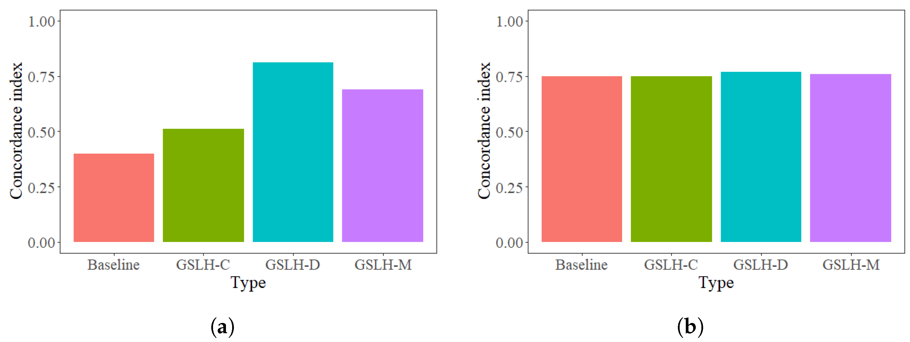
Based on the proposed formulation and estimation algorithm, the tripartite method for handling group-shared missing covariates can be further developed. The existence of GSLH is examined via comparing the DIC statistics of Markov chain Monte Carlo (MCMC) simulations between the proposed model and the baseline model which fails to consider multi-type GSLH. The DIC differences between the proposed model and the baseline model serve as the estimates of the expected loss differences in prediction. A negative value indicates that the proposed model with GSLH is more effective at capturing the underlying patterns of lifetime data; thus, the existence of GSLH should be considered. The correct type of GSLH can then be identified based on different structures of group-shared missing covariates. The proposed model with the correct type of GSLH is expected to achieve the best model-fitting performance. With the identified model, we can derive both point estimates and interval estimates of model parameters, enabling the quantification of the influence of both observed and group-shared missing covariates. With the identified missing information, we can also collaborate with the data provider to pinpoint the group-shared missing covariates with convincing interpretations based on available domain knowledge. Such a systematic process is performed iteratively until all group-shared missing information has been thoroughly explored.

With the derived estimates of unknown model parameters $\Theta$ and the cases of multi-type GSLH $W_i$ as well as hyper-parameters, we can further calculate the reliability function. Given a test unit l at time $T_c$, the estimated reliability function can be expressed as $\widehat{R}(T_c\mid \Theta ,W_l,\mathit{D})=1-{\int }_0^{T_c}f(s\mid \widehat{\Theta },{\widehat{W}}_l,\mathit{D})\mathrm{d}s$, where $\widehat{\Theta }$ and ${\widehat{W}}_l$ can be drawn from the derived conditional posteriors, as elaborated in Section 4.1, Section 4.2 and Section 4.3.

4.5. Discussion

We can delineate various specifications for the distribution of random error ${ϵ}_{ij}$, as shown in Equation (2). In this paper, the commonly used normal distribution and the extreme value distribution are selected for illustration purposes. By employing the reparameterization technique, the proposed model with a discrete type of GSLH is reduced to the log-normal mixture model and the Weibull mixture model, respectively [27]. The following proposition clarifies such a model reduction.

Proposition 1.

When ${ϵ}_{ij}$ is specified with different distributions, the GSLH-D model is reduced to the log-normal mixture model or the Weibull mixture model with specific unknown parameters ${\Theta }_k$ for each subpopulation $k,\forall k=1,\cdots ,K$, i.e., $f(t\mid \Theta )={\sum }_{k=1}^K{p}_k{f}_k(t\mid {\Theta }_k)$, where t is the product lifetime, and $f_k\left(·\right)$ represents the Weibull density function or the log-normal density function for the product lifetime of the units belonging to the subpopulation k. Specifically,

• When ${ϵ}_{ij}$ follows a normal distribution, i.e., ${ϵ}_{ij}=\sigma {\eta }_{ij}$, where ${\eta }_{ij}$ is a standard normal random variable and $\sigma >0$. Furthermore, we denote the unknown parameters related to the subpopulation k as ${\Theta }_k=\{{\mu }_k,{\sigma }_k^2\}$, where ${\mu }_k$ and ${\sigma }_k^2$ represent the mean and the variance on a logarithmic scale, respectively. Then, the GSLH-D model degenerates into the log-normal mixture model, i.e., $f\left(t\right)={\sum }_{k=1}^K{p}_{k}LN({\mu }_k={\beta }_0+{\mathit{\beta }}^{\mathrm{T}}{\tilde{\mathit{x}}}_{ij}+d_k,{\sigma }_k^2={\sigma }^2)$.
• When ${ϵ}_{ij}$ follows an extreme value distribution, i.e., ${ϵ}_{ij}=\sigma {\eta }_{ij}$, where ${\eta }_{ij}$ is a random variable with standard Gumbel distribution and $\sigma >0$. Furthermore, we denote the unknown parameters related to the subpopulation k as ${\Theta }_k=\{{\lambda }_k,{\rho }_k\}$, where ${\lambda }_k$ and ${\rho }_k$ are the rate and shape parameters, respectively. Then, the GSLH-D model degenerates into the Weibull mixture model, i.e., $f\left(t\right)={\sum }_{k=1}^K{p}_{k}Weib({\lambda }_k=exp[-\frac{1}{\sigma }({\beta }_0+{\mathit{\beta }}^{\mathrm{T}}{\tilde{\mathit{x}}}_{ij}+d_k)],{\rho }_k=\frac{1}{\sigma })$.

Proposition 1 implies that the baseline hazard, which captures the underlying risk without considering the influence of any covariates, would become specific to each subpopulation rather than being shared across multiple different subpopulations. The discrete type of GSLH can then be captured by the subpopulation-specific model parameters ${\Theta }_k$. The detailed proof can be found in Appendix A.

Moreover, with the derived conditional posteriors of multi-type GSLH, we can obtain the following insights. First, in the GSLH-D model, all data of the same subpopulation contributes to the estimation of $W_i$. The Bayesian framework enables information sharing among different product units from different groups that belong to the same subpopulation, and a large sample size is not required. On the other hand, only data within the same group is effective for the estimation of GSLH in the GSLH-C and GSLH-M models. Furthermore, the GSLH-M model with a more complex covariate structure is closely connected to the GSLH-D and GSLH-C models. When $W_i$ within each subpopulation approximately follows a degenerate distribution (i.e., subpopulation-specific $W_i$ is close to a constant value), the model with a mixed-type GSLH demonstrates similarities to the model with a discrete type of GSLH. When the entire population consists of a single subpopulation, the model with a mixed-type GSLH becomes the same as the model with continuous type of GSLH.

5. Case Study

To validate the proposed lifetime modeling and prediction framework with multi-type GSLH, we conduct a comprehensive simulation study and a real case study in Section 5.1 and Section 5.2, respectively.

5.1. A Simulation Study

5.1.1. Experimental Setting

We first conduct a simulation study using ground truth settings to thoroughly explore various types of GSLH and assess the performance of the proposed approach in comparison with alternative approaches. For the purpose of illustrating GSLH, we focus on two distinct subpopulations (i.e., $K=2$) and specify a total proportion of 0.35 for subpopulation 1. For each type of GSLH, the continuous component is generated randomly based on a normal distribution. In this work, we investigate two distinct model specifications, namely, the log-normal and the Weibull models, without losing generality. Figure 3 shows various structures of missing covariates shared within each group in the log-normal model. The scenarios $S_1$–$S_3$ refer to the simulation scenarios of the discrete type, mixed-type, and continuous type of group-shared missing covariates, respectively. As shown in Figure 3, it becomes less identifiable among different subpopulations from $S_1$ to $S_3$, and the discrete part eventually diminishes in $S_3$. In the simulation study, we consider a single observed covariate and uniformly generate the covariate data. To demonstrate the modeling effectiveness under small sample size, we create a simulation scenario with ten groups and five sample units per group using different types of GSLH (i.e., $S_1$, $S_2$, and $S_3$) to examine the model performance. Furthermore, to investigate the impact of number of groups n and sample size per group M on the model robustness, we create two more simulation settings via enlarging n and M, respectively (i.e., $n=100$, $M=5$ and $n=10$, $M=20$).

To implement the proposed estimation algorithm, informative priors are assigned to the majority of unknown parameters, facilitating the effective learning of data patterns. We ran two independent MCMC chains with 50,000 iterations each, following a burn-in period of 10,000 iterations. The convergence of the proposed algorithm is examined via the potential variance scale reduction factor [34]. The developed algorithm achieves an approximate convergence with a monitoring value of less than 1.1. The potential scale reduction factor is a measure indicating how much between-chain variation might decrease in future simulations. A potential scale reduction factor of 1.1 suggests a limited gain in inferential precision by prolonging chain runs. However, the dynamics of MCMC mean that between-chain variance can decrease before increasing. If the initial simulation pulls all chains to the distribution center, they may disperse again with further simulation. Furthermore, we implement the tripartite method to handle the group-shared missing covariates. In this work, the model without considering the influence of group-shared missing covariates is used as the baseline. The DIC differences between the proposed model and the baseline model are calculated, and the negative values further imply the existence of GSLH. We then identify the type of GSLH via comparing model-fitting performances. The model with the correct type of GSLH is expected to achieve the largest performance improvement [28]. To specify the density of the continuous component for the GSLH-C and GSLH-M models, we consider the normal, exponential, and gamma densities, which are commonly used in reliability analysis [21,24]. We select the density specification that has the potential to achieve the best model performance. Moreover, the number of subpopulations for the GSLH-D and GSLH-M models can be determined in a similar manner. With the identified model structure, we can further quantify the influence of group-shared missing covariates.

5.1.2. Parameters Estimation and Performance Evaluation

Both the posterior mean and the 95% credible interval of the estimated GSLH with log-normal and Weibull specifications are calculated and illustrated in Figure 4. As shown in each graph of Figure 4, the horizontal axis is a group index that is an index representing the unit j within the group i, and the vertical axis is $W_i$. The point estimates and the interval estimates are obtained simultaneously via the developed Bayesian estimation procedure. As depicted in Figure 4, the posterior means of the estimated GSLH are close to the ground truth values. Moreover, if the model is correctly specified, it is noteworthy that the 95% credible intervals entirely cover the true values. To the contrary, the conventional MLE approach [30] fails to provide either point estimates or interval estimates for the multi-type GSLH. Although some marginalized approaches with data augmentation [36] could derive the approximated interval estimates, they mainly rely on asymptotic approximations with large samples [37], which may not be practical for real-world scenarios. The proposed work demonstrates its ability to quantify the exact uncertainty of GSLH and the influence of multi-type group-shared missing covariates, even under limited sample sizes. Moreover, the proposed approach can quantify the effects of observed covariates under different scenarios of missing covariate information, even when the sample size per group is small, as shown in Figure 5. The posterior mode of the estimated coefficient of the observed covariate is close to the ground truth value under all simulation scenarios.

Furthermore, we investigate how the sample size would affect model estimation performance. Specifically, we use the GSLH-C model with both log-normal and Weibull specifications under different settings of sample size in scenario $S_3$ as an illustration example. As shown in Figure 6, the derived 95% credible intervals completely encompass the true values in all settings. In the illustrated group, the standard deviation of the estimated GSLH decreases when sample size per group increases. In addition to the improved precision, the posterior mode of the estimated GSLH approaches closer to the true value when M becomes larger. This is because the group-specific data contributes to the estimation of GSLH, as shown in Equation (11). The estimation performance among all groups are further illustrated in Figure 7. When sample size M increases, the estimation accuracy of GSLH is improved with significantly decreased bias.

5.1.3. Lifetime Prediction and Performance Evaluation

Based on the estimated models, we further conducted lifetime prediction along with performance evaluation. Specifically, the Kaplan–Meier (K–M) survival curves [38] were calculated to evaluate the prediction performance of the proposed approach in comparison with alternative methods. The reliability curve computed from the actual data was used as the benchmark. To explore the significance of properly handling multi-type missing covariates shared within each group, we compare the predicted reliability curves evaluated at new values of the observed covariates among the proposed approach and the conventional methods that neglect group-shared missing information. As illustrated in Figure 8, the predicted K–M curves based on the proposed approach with both log-normal and Weibull specifications are close to those of the actual data. On the other hand, the conventional methods tend to either overestimate or underestimate the reliability curve, as shown in Figure 8. As compared with the proposed approach, the alternative methods that neglect the positive effects of group-shared missing covariates lead to an underestimation of the K–M curve and vice versa. Overall, the proposed framework is demonstrated to achieve both improved estimation performance and lifetime prediction performance with different specifications in various simulation scenarios.

5.1.4. Model Robustness Evaluation

Based on the above results, the proposed work demonstrates its effectiveness in quantifying the influence of group-shared missing covariates with improved performance given that the underlying covariate structure is correctly specified. However, the missing covariate information is typically unknown in real-world practice. Therefore, we further investigate the model robustness in the presence of misspecification issues among different simulation scenarios and simulation settings. We denote $\Delta$ as the DIC difference between the baseline homogeneous model and the evaluated model. As a lower DIC value signifies an improved goodness-of-fit performance, a larger $\Delta$ then implies a better performance improvement of the assessed model in comparison with the baseline. The empirical results of the proposed model with log-normal specification are summarized in

Table 1. Performance comparison results with log-normal specification.

Settings			GSLH-C		GSLH-D		GSLH-M
			$\Delta$	$\mathit{\iota }$ (%)	$\Delta$	$\mathit{\iota }$ (%)	$\Delta$	$\mathit{\iota }$ (%)
$S_1$	$n=10$	$M=5$	95.96	75.14	386.03	0	282.12	26.92
	$n=10$	$M=20$	803.15	48.72	1566.12	0	1280.62	18.23
	$n=100$	$M=5$	1718.82	56.28	3931.19	0	3497.82	11.02
$S_2$	$n=10$	$M=5$	86.31	81.08	209.56	54.07	456.26	0
	$n=10$	$M=20$	758.56	58.87	841.44	54.38	1844.38	0
	$n=100$	$M=5$	1778.96	60.89	1954.08	57.04	4548.78	0
$S_3$	$n=10$	$M=5$	327.03	0	38.09	88.35	122.54	62.53
	$n=10$	$M=20$	1675.17	0	188.49	88.75	819.64	51.07
	$n=100$	$M=5$	4350.94	0	412.18	90.53	1843.55	57.63

. The adequate model in each scenario (i.e., GSLH-D in $S_1$, GSLH-M in $S_2$, and GSLH-C in $S_3$) achieves the best goodness-of-fit performance improvement with the largest $\Delta$ among all evaluated models. Furthermore, the suggested lifetime model would be reduced to the frailty model [21] under GSLH-C in $S_3$. The proposed work effectively deals with the multi-type group-shared missing covariates and demonstrates its ability to discern the accurate type of GSLH, particularly concerning the discrete type and the mixed-type, which have not been thoroughly investigated in prior research.

Moreover, we evaluate model-fitting performance under a misspecification issue. We denote $\iota (\%)$ as the scaled difference of performance improvements between the evaluated model and the model with the correct type of GSLH, which indicates the performance loss due to model misspecification. A smaller $\iota (\%)$ implies that the evaluated model is less sensitive to the misspecification issue and can retain more performance improvement. When the GSLH-D model is misspecified (i.e., in $S_2$ and $S_3$), the performance loss $\iota (\%)$ becomes larger when n or M increases. The enlarged subpopulation data that contributes to the estimation of GSLH makes the GSLH-D model more sensitive to the misspecification issue and induces more performance loss. Moreover, the GSLH-C model is susceptible to the model misspecification issue with significantly large $\iota (\%)$ in $S_1$ and $S_2$, as shown in Table 1. When the sample size per group increases, the performance loss of the misspecified GSLH-C slightly decreases. Moreover, the empirical results show that the GSLH-M model exhibits more robustness under model misspecification with slightly smaller $\iota (\%)$ as compared with the other misspecified model (i.e., GSLH-C in $S_1$ and GSLH-D in $S_3$). The proposed model with Weibull specification exhibits similar results, as shown in

Table 2. Performance comparison results with Weibull specification.

Settings			GSLH-C		GSLH-D		GSLH-M
			$\Delta$	$\mathit{\iota }$ (%)	$\Delta$	$\mathit{\iota }$ (%)	$\Delta$	$\mathit{\iota }$ (%)
$S_1$	$n=10$	$M=5$	92.04	53.69	198.78	0	184.02	7.43
	$n=10$	$M=20$	372.74	52.99	792.91	0	781.44	1.45
	$n=100$	$M=5$	1008.19	49.59	2000.04	0	1877.39	6.13
$S_2$	$n=10$	$M=5$	91.21	50.34	149.29	18.71	183.65	0
	$n=10$	$M=20$	383.41	49.27	556.61	26.35	755.77	0
	$n=100$	$M=5$	963.46	48.61	1233.81	34.18	1874.53	0
$S_3$	$n=10$	$M=5$	172.21	0	88.06	48.86	152.94	11.19
	$n=10$	$M=20$	800.72	0	359.31	55.13	754.69	5.75
	$n=100$	$M=5$	1811.76	0	503.85	72.19	1253.61	30.81

. The model with the correct type of GSLH achieves the largest performance improvement. Furthermore, the GSLH-C and GSLH-D models induce more performance loss as compared with the GSLH-M model under the misspecification issue. The GSLH-D model exhibits more vulnerability with increased sample size per group or number of groups. Additionally, the misspecified GSLH-C model exhibits more robustness when the sample size per group increases.

Furthermore, we evaluate the estimation robustness of GSLH in the presence of a misspecification issue among different settings of n and M. We use the posterior mean error to evaluate the estimation accuracy of GSLH, which is computed by the average of absolute differences between the posterior means and the actual values. The empirical results of the posterior mean error based on the proposed approach with both log-normal and Weibull specifications in various scenarios under diverse simulation settings are depicted in Figure 9. The model with the correct type of GSLH achieves the highest estimation accuracy, which is highlighted in green. For the adequate model in each scenario, the posterior mean error of the GSLH-D model decreases when either M or n increases, while the posterior mean error of the GSLH-C or GSLH-M model decreases only when the sample size per group increases. The misspecified model with the lowest estimation accuracy in each scenario is highlighted in red, as shown in Figure 9. The GSLH-M model has better estimation accuracy as compared with the GSLH-C or GSLH-D models when the type of GSLH is misspecified. We further empirically investigate the impact of n and M on the estimation accuracy of the assessed model in the presence of a misspecification issue. As shown in Figure 9, when the GSLH-D model is misspecified in $S_2$, where the ground truth GSLH involves both discrete and continuous components, a larger M could slightly improve the estimation accuracy. However, when the ground truth GSLH is purely continuous in scenario $S_3$, the estimation robustness of the misspecified GSLH-D model deteriorates with increased subpopulation data. Moreover, when the GSLH-C model is misspecified (e.g., in $S_1$ and $S_2$), the estimation accuracy could be improved when M becomes larger, as illustrated in Figure 9. Such an empirical conclusion also holds for the misspecified GSLH-M model in scenario $S_1$ and $S_3$.

5.2. A Real Case Study

To further exemplify the practical applicability of the proposed work, we carried out a real case study on the lifespan analysis of molding material units. In a tensile test, the test unit was subjected to the controlled tensile forces, generating stress–strain data. The data were collected by advanced instrumentation, including strain gauges and load cells. The stress–strain data captures the unit-level response to the applied strain level and provides valuable insights into mechanical properties of the material units. A total of 36 tensile tests are conducted, from which we obtain the actual lifespans of the test units using the stress–strain data [39]. Due to confidentiality concerns, the configuration details of the tensile tests are not accessible in the initial study.

To examine whether there is missing information shared within each batch, the tripartite method is utilized to analyze the lifetime data. The DIC differences between the proposed approach with multi-type GSLH and the baseline model without considering GSLH are calculated to examine the existence of group-shared missing covariates. All DIC differences are smaller than −100 for different types of GSLH, indicating that GSLH should be considered in the analysis of lifetime data. To further identify the type of GSLH and the structure of group-shared missing covariates, we compare the model-fitting performance among the proposed models with different types of GSLH. The DIC improvements between the evaluated models and the baseline homogeneous model are calculated as the identification metric. As shown in Figure 10a, the GSLH-D model achieves the greatest performance improvement as compared with the others (e.g., GSLH-C and GSLH-M). This indicates that the underlying missing covariates shared within each batch are more likely to be categorical. We then consulted domain experts and extracted additional knowledge about such influential group-shared missing covariates, which tend to be discrete in nature. We inform that different ordinal levels of tensile forces (i.e., low and high) have been applied to different batches of test units during the tensile test. By incorporating such discrete group-shared covariates, we then examine whether there is any other potential missing covariate information shared within each batch. The slight positive values of DIC differences between the proposed approach and the baseline model indicate that a substantial portion of the latent heterogeneity has been explained by the observed covariates, as shown in Figure 10b. Further incorporation of GSLH does not provide significant values in uncovering useful patterns of lifetime data.

Furthermore, we used the proposed approach to quantify the effects of such missing covariates shared within each batch on lifetime data. As shown in Figure 11, the estimated quantities of GSLH in the initial study can almost capture the covariate effects in the further exploration when the covariate information is incorporated. Moreover, we evaluate the effectiveness of the proposed approach based on the concordance index (C-index) [40], which is a useful metric for assessing the concordance between the observations and the predictions in time-to-event data analysis. A value exceeding 0.7 implies the appropriateness of the evaluated model for analyzing lifetime data. As shown in Figure 12a, the C-index of the proposed model with the identified discrete type of GSLH exceeds 0.8, implying a strong model for capturing lifetime data patterns, even in the absence of covariate information. The prediction power of the identified GSLH-D model surpasses those of the other models, which validates the effectiveness of the proposed approach. Moreover, when the uncovered group-shared covariates are incorporated into the lifetime model, the prediction power scores are comparable among the baseline model and the proposed models with different types of GSLH, as illustrated in Figure 12b. The difference between the proposed model and the baseline model becomes slight when the covariate information is incorporated. Nevertheless, the uncovered group-shared covariates could only explain part of the variations, and more investigations are needed to further improve the modeling performance.

Overall, the proposed approach demonstrates its ability to handle group-shared missing covariates in this pilot study. The empirical results can guide the reliability engineer in uncovering important missing covariate information and incorporating such group-shared covariates to improve the reliability assessment. Moreover, the quantified influence of group-shared missing covariates can shed light on identifying the most appropriate design changes during the design stage.

6. Conclusions

We proposed a flexible lifetime modeling and prediction approach with multi-type GSLH to account for the influence of complex group-shared missing covariates on product lifetime. Specifically, we first proposed a new lifetime model to comprehensively investigate multiple different structures of group-shared missing covariates. Bayesian estimation algorithms and inference procedures were further developed to simultaneously quantify the influence of both observed covariates and multi-type missing covariates shared within each group. With the generic formulation and effective estimation algorithms, a tripartite method was then developed to handle the multi-type group-shared missing covariates in a practical product lifetime analysis. The existence of multi-type group-shared missing covariates was first examined via a DIC statistics comparison. The correct type of the detected missing covariates was further identified, and finally, the influence of the group-shared missing covariates were quantified. A comprehensive simulation study was conducted under different scenarios of missing covariate information. The proposed approach showcases its effectiveness at handling multi-type group-shared missing covariates, leading to a substantial enhancement in estimation performance and prediction accuracy. Moreover, we investigated model robustness in the presence of misspecification issues. Furthermore, a real case study was presented to illustrate the applicability of the proposed work for uncovering the potential structure of multi-type group-shared missing covariates and alleviating the impact of missing covariate information on practical analysis of product lifetime. After further consultation with the data provider based on the identified information, the group-shared covariates can then be revealed with compelling interpretability.

In this paper, a novel lifetime modeling and prediction approach for a single-component system was developed. An interesting future research topic is to develop reliability analysis methods for multi-component systems with the intricate challenges posed by multi-type group-shared missing covariates. Moreover, the primary focus of this work centered on product lifetime analysis in the presence of group-shared missing covariates. Another promising direction is to develop degradation models for handling such multi-type group-shared missing information in product degradation analysis. In addition, the proposed work can be extended to semi-parametric models, such as Cox proportional hazards models for survival analysis in the future as well.

References

1. Zhu, W.; Fouladirad, M.; Bérenguer, C. Condition-based maintenance policies for a combined wear and shock deterioration model with covariates. Comput. Ind. Eng. 2015, 85, 268–283. [Google Scholar] [CrossRef]
2. Zhuang, L.; Xu, A.; Pang, J. Product reliability analysis based on heavily censored interval data with batch effects. Reliab. Eng. Syst. Saf. 2021, 212, 107622. [Google Scholar] [CrossRef]
3. Zhu, M.; Zhou, X. Lifecycle maintenance scheduling of station with multiple categories of information. Comput. Ind. Eng. 2022, 172, 108593. [Google Scholar] [CrossRef]
4. Cha, J.H.; Finkelstein, M. Some notes on unobserved parameters (frailties) in reliability modeling. Reliab. Eng. Syst. Saf. 2014, 123, 99–103. [Google Scholar] [CrossRef]
5. Moazeni, M.; Behbahani, M.; Khedmati, M.; Niaki, S.T.A. Single-replicate longitudinal data analysis in the presence of multiple instrumental measurement errors. Comput. Ind. Eng. 2020, 141, 106301. [Google Scholar] [CrossRef]
6. Liu, Y.; Dillon, T.; Yu, W.; Rahayu, W.; Mostafa, F. Missing value imputation for industrial IoT sensor data with large gaps. IEEE Internet Things J. 2020, 7, 6855–6867. [Google Scholar] [CrossRef]
7. García-Mora, B.; Debón, A.; Santamaría, C.; Carrión, A. Modelling the failure risk for water supply networks with interval-censored data. Reliab. Eng. Syst. Saf. 2015, 144, 311–318. [Google Scholar] [CrossRef]
8. Jeon, J.; Sohn, S.Y. Product failure pattern analysis from warranty data using association rule and Weibull regression analysis: A case study. Reliab. Eng. Syst. Saf. 2015, 133, 176–183. [Google Scholar] [CrossRef]
9. Evanschitzky, H.; Eisend, M.; Calantone, R.J.; Jiang, Y. Success factors of product innovation: An updated meta-analysis. J. Prod. Innov. Manag. 2012, 29, 21–37. [Google Scholar] [CrossRef]
10. Lauvernet, C.; Helbert, C. Metamodeling methods that incorporate qualitative variables for improved design of vegetative filter strips. Reliab. Eng. Syst. Saf. 2020, 204, 107083. [Google Scholar] [CrossRef]
11. Marmor, Y.N.; Bashkansky, E. Processing new types of quality data. Qual. Reliab. Eng. Int. 2020, 36, 2621–2638. [Google Scholar] [CrossRef]
12. Jones, B.; Jenkinson, I.; Yang, Z.; Wang, J. The use of Bayesian network modelling for maintenance planning in a manufacturing industry. Reliab. Eng. Syst. Saf. 2010, 95, 267–277. [Google Scholar] [CrossRef]
13. Johnen, M.; Schmitz, C.; Kateri, M.; Kamps, U. Fitting lifetime distributions to interval censored cyclic-aging data of lithium-ion batteries. Comput. Ind. Eng. 2020, 143, 106418. [Google Scholar] [CrossRef]
14. Okaro, I.A.; Tao, L. Reliability analysis and optimisation of subsea compression system facing operational covariate stresses. Reliab. Eng. Syst. Saf. 2016, 156, 159–174. [Google Scholar] [CrossRef]
15. Yao, Y.; Yao, N.; Zhou, X.; Li, Z.; Yue, X.; Yan, C.; Zhang, Q. Ethylene-carbonate-free electrolytes for rechargeable Li-ion pouch cells at sub-freezing temperatures. Adv. Mater. 2022, 34, 2206448. [Google Scholar] [CrossRef] [PubMed]
16. Antony Samy, A.; Golbang, A.; Harkin-Jones, E.; Archer, E.; Dahale, M.; McIlhagger, A. Influence of ambient temperature on part distortion: A simulation study on amorphous and semi-crystalline polymer. Polymers 2022, 14, 879. [Google Scholar] [CrossRef] [PubMed]
17. Meeker, W.Q.; Escobar, L.A.; Pascual, F.G. Statistical Methods for Reliability Data; John Wiley & Sons: Hoboken, NJ, USA, 2022. [Google Scholar]
18. Kong, D.; Huang, J.; Balakrishnan, N.; Cui, L. Stochastic quantile-filling augmentation algorithm to censored and accurate reliability data. Comput. Ind. Eng. 2017, 108, 27–38. [Google Scholar] [CrossRef]
19. Si, W.; Yang, Q.; Monplaisir, L.; Chen, Y. Reliability analysis of repairable systems with incomplete failure time data. IEEE Trans. Reliab. 2018, 67, 1043–1059. [Google Scholar] [CrossRef]
20. Zhou, R.; Li, H.; Sun, J.; Tang, N. A new approach to estimation of the proportional hazards model based on interval-censored data with missing covariates. Lifetime Data Anal. 2022, 28, 335–355. [Google Scholar] [CrossRef]
21. Deep, A.; Veeramani, D.; Zhou, S. Event prediction for individual unit based on recurrent event data collected in teleservice systems. IEEE Trans. Reliab. 2019, 69, 216–227. [Google Scholar] [CrossRef]
22. Ye, Z.S.; Hong, Y.; Xie, Y. How do heterogeneities in operating environments affect field failure predictions and test planning? Ann. Appl. Stat. 2013, 7, 2249–2271. [Google Scholar] [CrossRef]
23. Slimacek, V.; Lindqvist, B. Reliability of wind turbines modeled by a Poisson process with covariates, unobserved heterogeneity and seasonality. Wind Energy 2016, 19, 1991–2002. [Google Scholar] [CrossRef]
24. Brito, É.S.; Tomazella, V.L.; Ferreira, P.H. Statistical modeling and reliability analysis of multiple repairable systems with dependent failure times under perfect repair. Reliab. Eng. Syst. Saf. 2022, 222, 108375. [Google Scholar] [CrossRef]
25. Morita, L.H.; Tomazella, V.L.; Balakrishnan, N.; Ramos, P.L.; Ferreira, P.H.; Louzada, F. Inverse Gaussian process model with frailty term in reliability analysis. Qual. Reliab. Eng. Int. 2021, 37, 763–784. [Google Scholar] [CrossRef]
26. Seo, K.; Pan, R. Data analysis of step-stress accelerated life tests with heterogeneous group effects. IISE Trans. 2017, 49, 885–898. [Google Scholar] [CrossRef]
27. Li, M.; Liu, J. Bayesian hazard modeling based on lifetime data with latent heterogeneity. Reliab. Eng. Syst. Saf. 2016, 145, 183–189. [Google Scholar] [CrossRef]
28. Berg, A.; Meyer, R.; Yu, J. Deviance information criterion for comparing stochastic volatility models. J. Bus. Econ. Stat. 2004, 22, 107–120. [Google Scholar] [CrossRef]
29. Orbe, J.; Ferreira, E.; Núñez-Antón, V. Comparing proportional hazards and accelerated failure time models for survival analysis. Stat. Med. 2002, 21, 3493–3510. [Google Scholar] [CrossRef] [PubMed]
30. Zhang, S.; Zhai, Q.; Shi, X.; Liu, X. A Wiener Process Model With Dynamic Covariate for Degradation Modeling and Remaining Useful Life Prediction. IEEE Trans. Reliab. 2022, 72, 214–223. [Google Scholar] [CrossRef]
31. Liu, D.; Wang, S.; Zhang, C. Reliability estimation by fusing multiple-source information based on evidential variable and Wiener process. Comput. Ind. Eng. 2021, 162, 107745. [Google Scholar] [CrossRef]
32. Van Dyk, D.A.; Meng, X.L. The art of data augmentation. J. Comput. Graph. Stat. 2001, 10, 1–50. [Google Scholar] [CrossRef]
33. Plummer, M. JAGS: A program for analysis of Bayesian graphical models using Gibbs sampling. In Proceedings of the 3rd International Workshop on Distributed Statistical Computing, Vienna, Austria, 20–22 March 2003; Volume 124, pp. 1–10. [Google Scholar]
34. Vehtari, A.; Gelman, A.; Simpson, D.; Carpenter, B.; Bürkner, P.C. Rank-normalization, folding, and localization: An improved R for assessing convergence of MCMC (with discussion). Bayesian Anal. 2021, 16, 667–718. [Google Scholar] [CrossRef]
35. Calderhead, B. A general construction for parallelizing Metropolis- Hastings algorithms. Proc. Natl. Acad. Sci. USA 2014, 111, 17408–17413. [Google Scholar] [CrossRef]
36. Chen, S.; Lu, L.; Xiang, Y.; Lu, Q.; Li, M. A data heterogeneity modeling and quantification approach for field pre-assessment of chloride-induced corrosion in aging infrastructures. Reliab. Eng. Syst. Saf. 2018, 171, 123–135. [Google Scholar] [CrossRef]
37. Ibragimov, I.A.; Has’ Minskii, R.Z. Statistical Estimation: Asymptotic Theory; Springer Science & Business Media: Berlin, Germany, 2013; Volume 16. [Google Scholar]
38. Ruppert, T.; Csalodi, R.; Abonyi, J. Estimation of machine setup and changeover times by survival analysis. Comput. Ind. Eng. 2021, 153, 107026. [Google Scholar] [CrossRef]
39. Huo, J.; Zhu, D.; Hou, N.; Sun, W.; Dong, J. Application of a small-timescale fatigue, crack-growth model to the plane stress/strain transition in predicting the lifetime of a tunnel-boring-machine cutter head. Eng. Fail. Anal. 2017, 71, 11–30. [Google Scholar] [CrossRef]
40. Schmid, M.; Wright, M.N.; Ziegler, A. On the use of Harrell’s C for clinical risk prediction via random survival forests. Expert Syst. Appl. 2016, 63, 450–459. [Google Scholar] [CrossRef]
Figure 1. The proposed lifetime modeling and prediction framework.
Mathematics 12 00740 g001
Figure 2. Hierarchy of proposed lifetime model with multi-type GSLH.
Mathematics 12 00740 g002
Figure 3. Different types of group-shared missing covariates in the log-normal model. (a) S 1 ; (b) S 2 ; (c) S 3 .
Mathematics 12 00740 g003
Figure 4. Influence quantification of group-shared missing covariates with M = 5 and n = 10 for different scenarios: (a,d) S 1 ; (b,e) S 2 ; (c,f) S 3 .
Mathematics 12 00740 g004
Figure 5. Influence quantification of observed covariate with M = 5 and n = 100 . (a) Log-normal; (b) Weibull.
Mathematics 12 00740 g005
Figure 6. Density plot of the estimated GSLH under different simulation settings. (a) Log-normal GSLH-C in S 3 ; (b) Weibull GSLH-C in S 3 .
Mathematics 12 00740 g006
Figure 7. Estimation bias of GSLH among all groups under different settings. (a) Log-normal GSLH-C in S 3 ; (b) Weibull GSLH-C in S 3 .
Mathematics 12 00740 g007
Figure 8. Prediction performance comparison with simulation setting M = 5 , n = 10 , and different specifications: (ac) log-normal; (df) Weibull. (a) GSLH-D in S 1 ( W > 0 ); (b) GSLH-M in S 2 ( W > 0 ); (c) GSLH-C in S 3 ( W < 0 ); (d) GSLH-D in S 1 ( W > 0 ); (e) GSLH-M in S 2 ( W < 0 ); (f) GSLH-C in S 3 ( W < 0 ).
Mathematics 12 00740 g008
Figure 9. Posterior mean error comparisons under different settings (1: M = 5 , n = 10 , 2: M = 20 , n = 10 , 3: M = 5 , n = 100 ) in different scenarios: (ac) log-normal; (df) Weibull. (a) S 1 ; (b) S 2 ; (c) S 3 ; (d) S 1 ; (e) S 2 ; (f) S 3 .
Mathematics 12 00740 g009
Figure 10. Model performance comparison with a multi-type GSLH. (a) Initial investigation without the inclusion of group-shared covariate information; (b) subsequent analysis with the incorporation of group-shared covariate information.
Mathematics 12 00740 g010
Figure 11. Influences quantification of group-shared missing covariates.
Mathematics 12 00740 g011
Figure 12. Prediction power comparisons based on the C-index. (a) Influences quantification of group-shared missing covariates; (b) subsequent analysis with the incorporation of group-shared covariate information.
Mathematics 12 00740 g012