Investigation of the Fork–Join System with Markovian Arrival Process Arrivals and Phase-Type Service Time Distribution Using Machine Learning Methods

Abstract

This paper presents a study of fork–join systems. The fork–join system breaks down each customer into numerous tasks and processes them on separate servers. Once all tasks are finished, the customer is considered completed. This design enables the efficient handling of customers. The customers enter the system in a MAP flow. This helps create a more realistic and flexible representation of how customers arrive. It is important for modeling various real-life scenarios. Customers are divided into $K\ge 2$ tasks and assigned to different subsystems. The number of tasks matches the number of subsystems. Each subsystem has a server that processes tasks, and a buffer that temporarily stores tasks waiting to be processed. The service time of a task by the k-th server follows a PH (phase-type) distribution with an irreducible representation (${\beta }_k$, $S_k$), $1\le k\le K$. An analytical solution was derived for the case of $K=2$ when the input MAP flow and service time follow a PH distribution. We have efficient algorithms to calculate the stationary distribution and performance characteristics of the fork–join system for this case. In general cases, this paper suggests using a combination of Monte Carlo and machine learning methods to study the performance of fork–join systems. In this paper, we present the results of our numerical experiments.

1. Introduction

Queueing systems with data partitioning and resynchronization (generally accepted as fork–join systems) are natural models of various computer and communication systems, particularly systems that perform parallel computing, customer processing in distributed databases, and parallel disk access [1,2,3,4]. The key feature of these systems is that after a customer enters the system, it is divided into a particular set of K tasks that are serviced by K parallel servers. A customer leaves the system when all subsystems complete all customer tasks. Thus, tasks corresponding to the same customer are joined before departing the system, and, accordingly, the service time of a customer corresponds to the maximum time spent in the system by one of the tasks.

In the case of infinite buffer, difficulties arise in calculating the joint stationary distribution of queue lengths, even under the most straightforward assumptions about the nature of the input flow and service times. Finding such a distribution is the subject of [5], where the case $K=2$, infinite buffer to servers, stationary Poisson flow, and exponential distributions of service times are considered. For such a system, a functional equation for the generating function of the joint distribution of queue lengths is obtained, and questions of the asymptotic behavior of joint probabilities are investigated. The results of [5] are used in [6], where a formula is derived for the mean sojourn time in the mentioned system under the simplifying assumption that the service rates on both servers are equal. In [7], the authors consider a fork–join system with two subsystems and more general time distributions between hyperexponential arrivals and the Erlang distribution of service times.

Due to the complexity of the problem of finding the sojourn time distribution in fork–join systems, in most works, the authors limit themselves to analyzing only mean sojourn time [5,6,7,8], in particular, finding upper or lower bounds for this time [9,10,11]. The overview of research in this area until 2014 can be found in [12].

Extensive applications of fork–join systems not only in computing systems and networks with parallel services but also in other industries, including the banking sector, medicine [13,14], and some others [15,16,17,18], stimulated further research in this area. The authors in [19] considered a method for calculating the stationary distribution of a fork–join system with a Markovian arrival, $K\ge 2$ homogeneous servers characterized by an exponential service time distribution, and infinite buffer, which involves solving a nonlinear matrix integral equation and the truncation of the state space of the process describing the operation of the system. The main results are obtained for the case $K=2$. In [20], a fork–join system with parallel servicing of customers ($K=2$), Poisson input flow, and PH-distribution of service time is considered. The conditions for a stationary mode, the main characteristics of system performance, and analytical expressions for the lower and upper bounds of the mean sojourn time in the system are found. An analysis of more general cases of studying fork–join systems, particularly with an arbitrary distribution of service time, was carried out in the literature only using approximate methods [21,22,23,24]. In the articles [25,26], systems with multiple resources are explored. A distinctive feature of such systems is that tasks from the customer simultaneously occupy a random number of servers. It depends on the number of tasks in the customer. In the article [27], you can familiarize yourself with the use of neural networks for the analysis of fork–join systems and other complex problems of queuing theory (for example, [28,29]).

The previous review showed that, despite using $K=2$ and making basic assumptions about the input flow and service time, a detailed analytical solution for determining the stationary characteristics of a fork–join system was not found. This article is important because it analyzes a fork–join system, considering the different assumptions about input flows and service time distribution. This research holds significant practical and theoretical value, making it truly novel and original. This work holds both practical and theoretical significance, marking a crucial advancement in the field. For the case where $K=2$, we obtained analytical expressions for the probability of losses, average queue length, and the distribution function of the response time for the first time. If $K\ge 2$, a new method is created and used. This method combines machine learning and the Monte Carlo methods. It efficiently calculates the characteristics of a complex fork–join system on a large scale. It is particularly useful for building real systems that require effective parallel task management.

This paper considers the various architectures of fork–join systems in more general assumptions about input flow and the distribution of service times. Customers enter the system according to the Markovian arrival process (MAP). Service times have a phase distribution (PH distribution). We organized the article as follows. Section 2 presents the problem statement. Section 3 is devoted to implementing a mathematical algorithm for calculating the stationary distribution and characteristics for the particular case of a fork–join system with $K=2$ with an input $MAP$ flow and $PH$—service time distribution. Section 4 describes a method for solving the general problem of studying a fork–join system using simulation and machine learning methods. Section 5 presents the numerical results of the study.

2. Problem Statement

We consider a fork–join queueing system with $K\ge 2$ servers in parallel (see Figure 1). Customers enter the system in a Markovian arrival process ($MAP$), which is specified by the underlying process ${\nu }_t,t\ge 0,$ which is a Markov chain with the state space $\{0,1,\dots ,W\}$, and the matrices $D_0$ and $D_1.$ The non-diagonal entries of the matrix $D_0$ are the rates of transitions of the chain ${\nu }_t,t\ge 0,$ which are not accompanied by the generation of a customer, while the entries of the matrix $D_1$ are the rates of transitions of the chain which are accompanied by the generation of a customer. The matrix $D\left(1\right)=D_0+D_1$ represents an infinitesimal generator of the chain ${\nu }_t,t\ge 0.$ The arrival rate $\lambda$ is defined as $\lambda =\theta D_{1}e$, where $\theta$ is a vector of the stationary distribution of the process ${\nu }_t$, which is defined as the unique solution of the system of linear algebraic equations $\theta D\left(1\right)=0$, $\theta e=1$. Here and further, e is a column vector consisting of ones, and 0 is a row vector consisting of zeros. A more detailed description of the $MAP$ can be found, for example, in [30,31].

An arriving customer entering the system forks into K tasks to be served in K independent subsystems $G_1,G_2,\cdots ,G_k$. The service time of a task by the k-th server has a $PH$ (phase-type) distribution with an irreducible representation $({\mathsf{\beta }}_k,S_k)$. This means that the service process on the k-th server is managed by the Markov chain $m_t^{\left(k\right)},t\ge 0,$ with the state space $\{1,\cdots ,M^{\left(k\right)},M^{\left(k\right)}+1\},$ where the state $M^{\left(k\right)}+1$ is an absorbing one. The rates of transitions in the set of unessential states are given by the matrices $S_k$ and the transition rates to absorbing states are given by the vectors ${\mathit{S}}_0^{\left(k\right)}=-S_k\mathbf{e}$. More details about the $PH$ can be found, for example, in [31,32]. A customer that arrives when the buffer of one of the systems $G_i,i=1,2,\cdots ,K$ is full leaves the system without a service (it is considered to be lost). A customer accepted into the system leaves the system as soon as all servers complete their task services. Thus, tasks corresponding to the same customer are joined before departing the system.

The main stationary characteristics of the performance of the described fork–join system are found, including the sojourn time in the system, average queue lengths, and the loss probability of customers.

3. Study of the Characteristics of a Fork–Join System with Parallel Servicing of Tasks $(\mathbf{K}=\mathbf{2})$

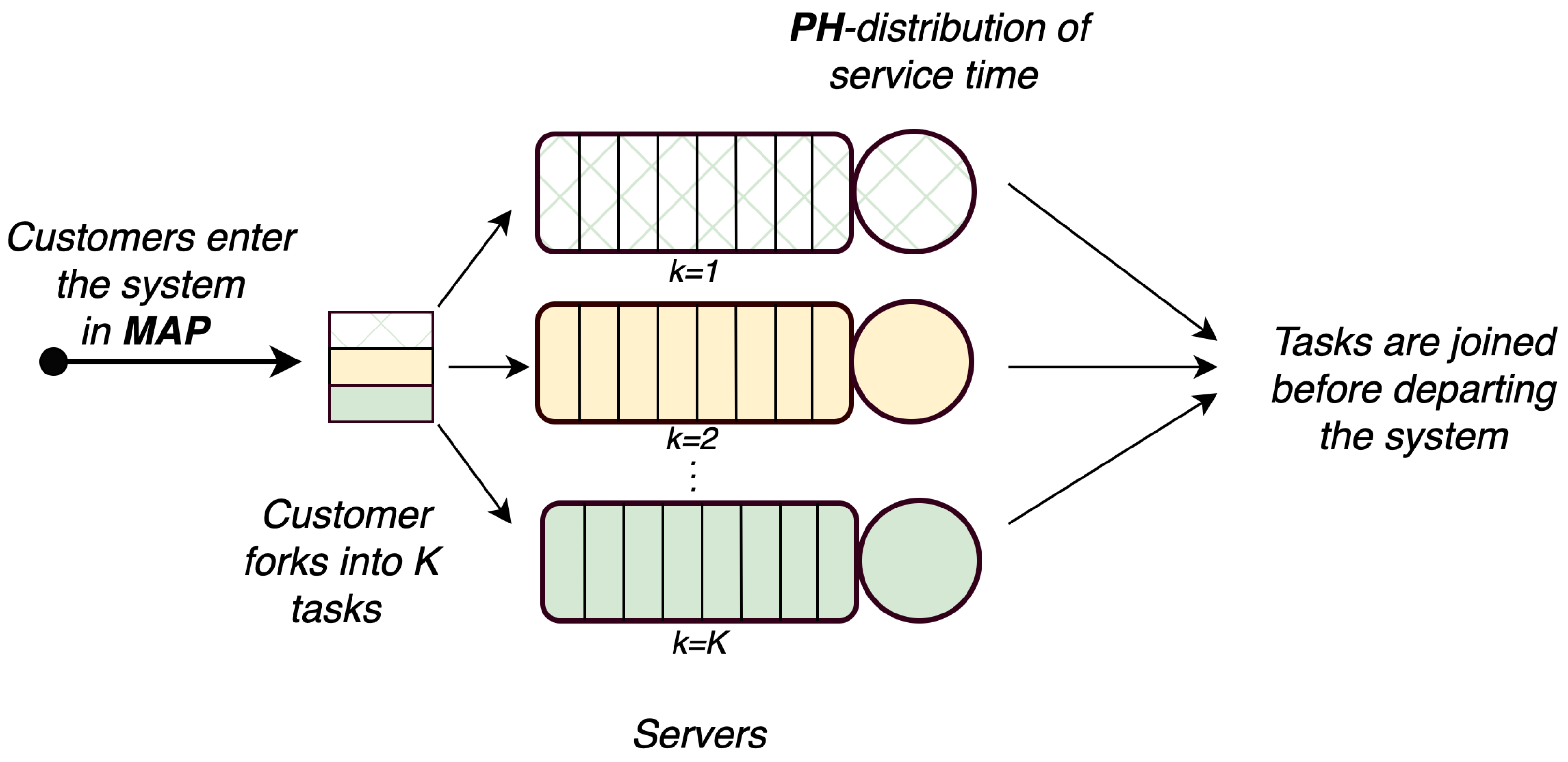
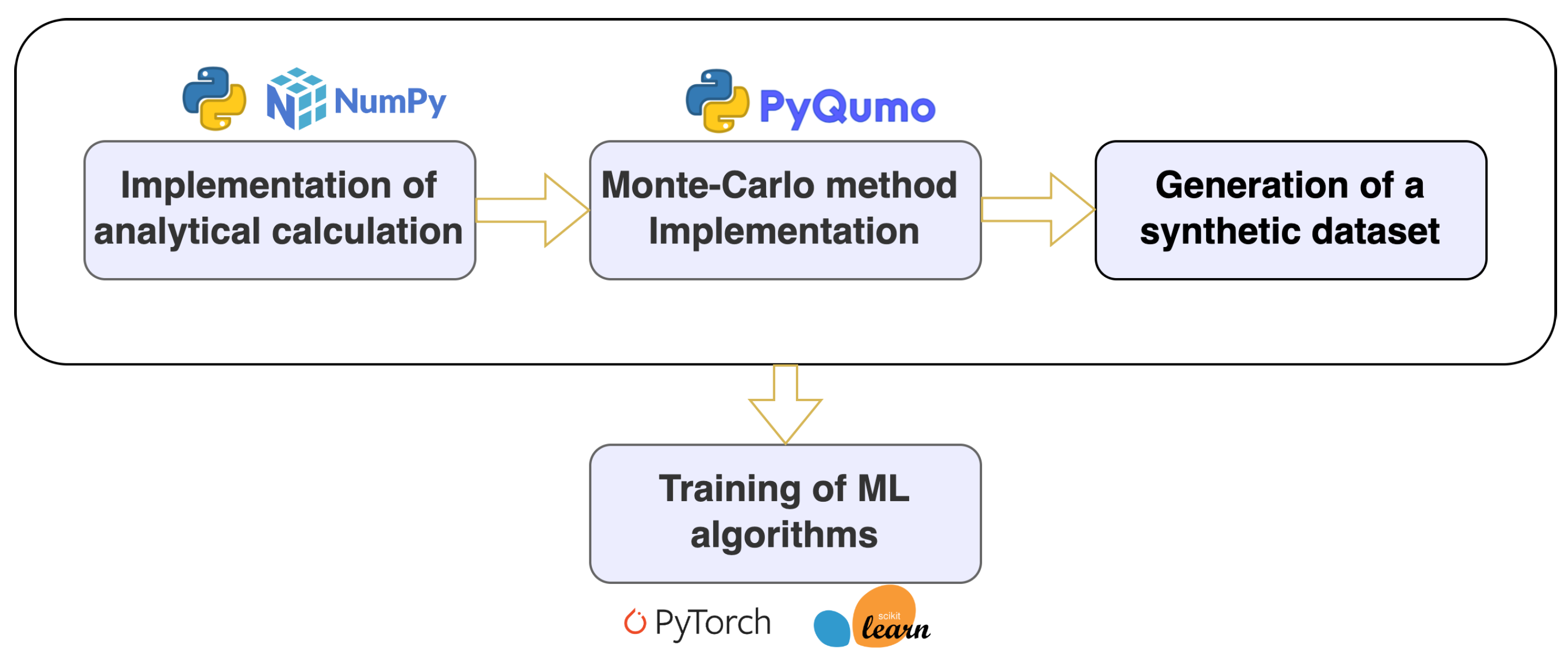
The analysis of this particular case is of theoretical interest, because the study of such a system under the assumption of an incoming $MAP$ flow and a $PH$ distribution of service time has not been previously considered in the literature. In addition, the numerical results of this section will be used to validate a simulation model that describes the functioning of the general fork–join system ($K\ge 2$) considered in this article.

3.1. Markov Chain Describing the Process of System Functioning

Assume that the first service device ($k=1$) has infinite buffer, and the capacity of the second ($k=2$) is limited.

At time t, let the following:

• $i_t$ denotes the number of tasks in the subsystem $G_1$, $i\ge 0$;
• $j_t$ denotes the number of tasks in the subsystem $G_2$, $j=\overline{0,J}$;
• ${\nu }_t$ denotes the states of the underlying process of the $MAP$, $v_t=\overline{0,W}$;
• $m_t^{\left(k\right)}$ denotes the states of underlying process of the $PH$ service process on the kth server, $m_t^{\left(k\right)}=\overline{1,M^{\left(k\right)}},$ $k=1,2.$

The operation of the system is described by a regular irreducible Markov chain ${\xi }_t,t\ge 0,$ with the state space

$$\Omega =\{(0,0,\nu ),\nu =\overline{0,W}\}\bigcup \{(i,0,\nu ,m^{\left(1\right)}),i>0,\nu =\overline{0,W},m^{\left(1\right)}=\overline{1,M^{\left(1\right)}}\}\bigcup$$

$$\{(0,j,\nu ,m^{\left(2\right)}),j=\overline{0,J},\nu =\overline{0,W},m^{\left(2\right)}=\overline{1,M^{\left(2\right)}}\}\bigcup$$

$$\{(i,j,\nu ,m^{\left(1\right)},m^{\left(2\right)}),i>0,j=\overline{1,J},\nu =\overline{0,W},m^{\left(1\right)}=\overline{1,M^{\left(1\right)}},m^{\left(2\right)}=\overline{1,M^{\left(2\right)}}\}.$$

Let us arrange the states of the chain ${\xi }_t$ in the lexicographic order and denote by $Q_{i,i^{\prime }}$ the matrix of transition rates of the chain from the states with the value i of the first component to the states with the value $i^{\prime }$ of this component. We also denote by $Q_r$ the matrix that is defined as $Q_r=Q_{i,i+r-1},i\ge 1,r\ge 0.$

To proceed to writing the infinitesimal generator Q of the Markov chain ${\xi }_t,t\ge 0,$ we introduce the following notations:

• I (O) is an identity (zero) matrix;
• $\overline{W}=W+1;$
• $\otimes (\oplus )$ is a symbol of the Kronecker product (sum) of matrices;
• $diag\{Z_l,l=\overline{1,L}\}$ is a diagonal matrix with diagonal blocks $Z_l$;
• $dia{g}^{-}\{Z_l,l=\overline{0,L}\}$ is a sub-diagonal matrix with sub-diagonal blocks $Z_l;$
• $dia{g}^{+}\{Z_l,l=\overline{0,L}\}$ is an over-diagonal matrix with over-diagonal blocks $Z_l;$

Lemma 1.

The infinitesimal generator Q of the Markov chain ${\xi }_t,t\ge 0$, has a block tridiagonal structure

$$Q=\left(\begin{array}{cccccc}{Q}_{0,0}& Q_{0,1}& O& O& O& \dots \\ Q_{1,0}& Q_1& Q_2& O& O& \dots \\ O& Q_0& Q_1& Q_2& O& \dots \\ O& O& Q_0& Q_1& Q_2& \dots \\ ⋮& ⋮& ⋮& ⋮& ⋮& \ddots \end{array}\right);$$

where non-zero blocks $Q_{i,i^{\prime }}$ have the following form:

• $Q_{0,0}$ is a square matrix of size $\overline{W}(1+J{M}_2),$

  $$Q_{0,0}=diag\{D_0,D_0\oplus S_2,D_0\oplus S_2,\dots ,D_0\oplus S_2,D\left(1\right)\oplus S_2\}+$$

  $$dia{g}^{-}\{I_{\overline{W}}\otimes {\mathit{S}}_0^{\left(2\right)},I_{\overline{W}}\otimes {\mathit{S}}_0^{\left(2\right)}{\mathsf{\beta }}_2,I_{\overline{W}}\otimes {\mathit{S}}_0^{\left(2\right)}{\mathsf{\beta }}_2,\dots ,I_{\overline{W}}\otimes {\mathit{S}}_0^{\left(2\right)}{\mathsf{\beta }}_2\};$$
• $Q_{0,1}$ is a matrix of size $\overline{W}(1+J{M}_2)\times \overline{W}{M}_1(1+J{M}_2),$

  $$Q_{0,1}=dia{g}^{+}\{D_1\otimes {\mathsf{\beta }}_1\otimes {\mathsf{\beta }}_2{D}_1\otimes {\mathsf{\beta }}_1\otimes I_{M_2},D_1\otimes {\mathsf{\beta }}_1\otimes I_{M_2},\dots ,D_1\otimes {\mathsf{\beta }}_1\otimes I_{M_2}\};$$
• $Q_{1,0}$ is a matrix of size $\overline{W}{M}_1(1+J{M}_2)\times \overline{W}(1+J{M}_2),$

  $$Q_{1,0}=diag\{I_{\overline{W}}\otimes {\mathit{S}}_0^{\left(1\right)},I_{\overline{W}}\otimes {\mathit{S}}_0^{\left(1\right)}\otimes I_{M_2},I_{\overline{W}}\otimes {\mathit{S}}_0^{\left(1\right)}\otimes I_{M_2},\dots ,I_{\overline{W}}\otimes {\mathit{S}}_0^{\left(1\right)}\otimes I_{M_2}\};$$
• $Q_0$ is a square matrix of size $\overline{W}{M}_1(1+J{M}_2),$

  $$Q_0=diag\{I_{\overline{W}}\otimes {\mathit{S}}_0^{\left(1\right)},I_{\overline{W}}\otimes {\mathit{S}}_0^{\left(1\right)}{\mathsf{\beta }}_1\otimes I_{M_2},I_{\overline{W}}\otimes {\mathit{S}}_0^{\left(1\right)}{\mathsf{\beta }}_1\otimes I_{M_2},\dots ,I_{\overline{W}}\otimes {\mathit{S}}_0^{\left(1\right)}{\mathsf{\beta }}_1\otimes I_{M_2}\};$$
• $Q_1$ is a square matrix of size $\overline{W}{M}_1(1+J{M}_2),$

  $$\begin{array}{ll}{Q}_1=& diag\{D_0\oplus S^{\left(1\right)},D_0\oplus S_1\oplus S_2,D_0\oplus S_1\oplus S_2,\dots ,D_0\oplus S_1\oplus S_2,D\left(1\right)\oplus S_1\oplus S_2\}+\\ & dia{g}^{-}\{I_{\overline{W}{M}_1}\otimes {\mathit{S}}_0^{\left(2\right)},I_{\overline{W}{M}_1}\otimes {\mathit{S}}_0^{\left(2\right)}{\mathsf{\beta }}_2,I_{\overline{W}{M}_1}\otimes {\mathit{S}}_0^{\left(2\right)}{\mathsf{\beta }}_2,\dots ,I_{\overline{W}{M}_1}\otimes {\mathit{S}}_0^{\left(2\right)}{\mathsf{\beta }}_2\};\end{array}$$
• $Q_2$ is a square matrix of size $\overline{W}{M}_1(1+J{M}_2),$

  $$Q_2=dia{g}^{+}\{D_1\otimes I_{M_1}\otimes {\mathsf{\beta }}_2,D_1\otimes I_{M_1{M}_2},D_1\otimes I_{M_1{M}_2},\dots ,D_1\otimes I_{M_1{M}_2}\}.$$

Proof. 

We represent each of the matrices $Q_{i,i^{\prime }}$ in the block form $Q_{i,i^{\prime }}={\left(Q_{i,i^{\prime }}\right)}_{j,j^{\prime }=\overline{0,J}}$ and explain the probabilistic meaning of their blocks.

The matrix $Q_{0,0}$ describes the rates of transitions of the Markov chain ${\xi }_t,t\ge 0,$ that do not lead to an increase in the number of tasks in the subsystems $G_1$ and $G_2$. In this matrix ${\left(Q_{0,0}\right)}_{j,j^{\prime }}=O,j^{\prime }>j,j^{\prime }<j-1,$ and the others blocks are described as follows:

${\left(Q_{0,0}\right)}_{0,0}$ contains the rates of transitions of the chain ${\xi }_t$ caused by the idle transitions of the $MAP$ (the rates are described by the matrix $D_0$);

${\left(Q_{0,0}\right)}_{j,j-1},j=\overline{1,J},$ contains the rates of transitions of the chain ${\xi }_t$ accompanied by the end of servicing on server 2 (the rates describe the matrix $I_{\overline{W}}\otimes {\mathit{S}}_0^{\left(2\right)},$ if $j=1,$ and the matrix $I_{\overline{W}}\otimes {\mathit{S}}_0^{\left(2\right)}{\mathsf{\beta }}_2,$ if $j>1$);

${\left(Q_{0,0}\right)}_{j,j},j=\overline{1,J-1},$ contains the rates of transitions of the chain ${\xi }_t,$ that do not lead to the arrival of a customer in the $MAP$ or the completion of the service on server 2. Such transitions are made during idle transitions of the underlying process $MAP$ or the underlying process of the service on server 2 (the rates are described by the matrix $D_0\oplus S_2$);

${\left(Q_{0,0}\right)}_{J,J}$ contains the rates of transitions of the chain ${\xi }_t$ that are caused by a change in the state of the underlying process of the $MAP$ (accompanied or not accompanied by the arrival of a customer) or idle transitions of the underlying process of the $PH$ service on server 2 (the rates are described by the matrix $D\left(1\right)\oplus S_2$);

The matrix $Q_{0,1}={\left(Q_{0,1}\right)}_{j,j^{\prime }=\overline{0,J}}$ describes the rates of transitions of the Markov chain ${\xi }_t$ which entail the arrival of a customer in the $MAP$. It has a block over-diagonal structure, where, for $j=0$, the over-diagonal blocks describe the transitions of the underlying process of the $MAP$ accompanied by the establishment of the initial phase of the service processes on the first and on the second servers (the matrix $D_1\otimes {\mathsf{\beta }}_1\otimes {\mathsf{\beta }}_2)$) or, for $0<j<J,$ transitions of the underlying process of the $MAP$ accompanied by the establishment of the initial phase of the service process on the first server and an increase in the queue in the system $G_2$ by one (the matrix $D_1\otimes {\mathsf{\beta }}_1\otimes I_{M_2}$).

The matrix $Q_{1,0}$ describes the rates of transitions of the Markov chain ${\xi }_t$ that lead to the completion of the service on the second server ((the rates are described by the matrix $I_{\overline{W}}\otimes {\mathit{S}}_0^{\left(1\right)},$ if $j=1,$ and by the matrix $I_{\overline{W}}\otimes {\mathit{S}}_0^{\left(1\right)}{\mathsf{\beta }}_1\otimes I_{M_2},$ if $j>1$);

The blocks $Q_0,Q_1,Q_2$ of the generator are described similarly to the blocks $Q_{1,0},Q_{0,0},Q_{0,1}$ but taking into account the fact that, at the time of the chain transition, the system $G_1$ is not empty.    □

Corollary 1.

The process ${\xi }_t,t\ge 0,$ belongs to the class of quasi- birth-and-death ($QBD$) processes. Proof of the corollary follows from the structure of the infinitesimal generator and the definition of a quasi- birth-and-death process given in [32].

3.2. Ergodicity Condition

The criterion for the existence of a stationary regime in the system under consideration coincides with the necessary and sufficient condition for the ergodicity of the Markov chain ${\xi }_t,t\ge 0$. This condition is defined in the following theorem.

Theorem 1.

The necessary and sufficient condition for the ergodicity of the Markov chain ${\xi }_t,t\ge 0,$ is the fulfillment of the inequality

$$\lambda (1-y_J\mathbf{e})<{\mu }_1,$$

(1)

where

$$y_J=\frac{{\left(\frac{\lambda }{{\mu }_2}\right)}^J/J!}{{\displaystyle \sum _{j=0}^J}{\left(\frac{\lambda }{{\mu }_2}\right)}^j/j!}.$$

(2)

Proof. 

According to [33], a necessary and sufficient condition for ergodicity is the fulfillment of the inequality

$$\mathbf{x}{Q}_2\mathbf{e}<\mathbf{x}{Q}_0\mathbf{e},$$

(3)

where the stochastic vector $\mathbf{x}$ is a solution to a system of linear algebraic equations

$$\mathbf{x}(Q_0+Q_1+Q_2)=\mathbf{0},$$

(4)

$$\mathbf{x}\mathbf{e}=1.$$

Let us represent the vector $\mathbf{x}$ in the form $\mathbf{x}=({\mathbf{x}}_0,{\mathbf{x}}_1,\dots ,{\mathbf{x}}_J)$, where the vector ${\mathbf{x}}_0$ has order an of $\overline{W}{M}_1$ and vectors ${\mathbf{x}}_j,j=\overline{1,J}$ have orders $\overline{W}{M}_1{M}_2.$ Then, taking into account the expressions for the blocks $Q_0,Q_1,Q_2$, specified in Lemma 1, the system (4) will be written as

$${\mathbf{x}}_0{A}_0+{\mathbf{x}}_1(I_{\overline{W}{M}_1}\otimes {\mathit{S}}_0^{\left(2\right)})=\mathbf{0}$$

$${\mathbf{x}}_{j-1}(D_1\otimes I_{M_1}\otimes {\mathsf{\beta }}_2)+{\mathbf{x}}_{j}A+{\mathbf{x}}_{j+1}(I_{\overline{W}{M}_1}\otimes {\mathit{S}}_0^{\left(2\right)}{\mathsf{\beta }}_2)=\mathbf{0},j=\overline{1,J-1},$$

(5)

$${\mathbf{x}}_{J-1}(D_1\otimes I_{M_1}\otimes {\mathsf{\beta }}_2)+{\mathbf{x}}_J(A+D_1\otimes I_{M_1{M}_2})=\mathbf{0},$$

where

$$A_0=I_{\overline{W}}\otimes (S_1+{\mathit{S}}_0^{\left(1\right)}{\mathsf{\beta }}_1)+D_0\otimes I_{M_1},$$

$$A=I_{\overline{W}}\otimes (S_1+{\mathit{S}}_0^{\left(1\right)}{\mathsf{\beta }}_1)\otimes I_{M_2}+D_0\otimes I_{M_1{M}_2}+I_{\overline{W}{M}_1}\otimes S_2.$$

Let us now represent the vectors ${\mathbf{x}}_j$ in the form ${\mathbf{x}}_0=\mathsf{\theta }\otimes {\mathbf{y}}_0,{\mathbf{x}}_j=\mathsf{\theta }\otimes {\mathbf{y}}_j\otimes {\mathsf{\delta }}_2,j=\overline{1,J},$ where $\mathsf{\theta }$ is the stationary vector of $MAP$, ${\mathsf{\delta }}_2$ is a stationary vector $P{H}_2,$ i.e., is the only solution to the system ${\mathsf{\delta }}_2(S_2+{\mathit{S}}_0^{\left(2\right)}{\mathsf{\beta }}_2)=\mathbf{0},{\mathsf{\delta }}_2\mathbf{e}=1$, and vectors ${\mathbf{y}}_j$ of order $M_1$ satisfy the normalization equation ${\displaystyle \sum _{j=0}^J}{\mathbf{y}}_j\mathbf{e}=1.$ We use these expressions in the equations of system (5), having previously multiplied the first equation by ${\mathbf{e}}_{\overline{W}}\otimes I_{M_1}$, and each of the subsequent equations on ${\mathbf{e}}_{\overline{W}}\otimes I_{M_1}\otimes {\mathbf{e}}_{M_2}.$

Taking into account the relations $\mathsf{\theta }\mathbf{e}=1,$ $-\mathsf{\theta }{D}_0\mathbf{e}=\mathsf{\theta }{D}_1\mathbf{e}=\lambda$, ${\mu }_2={\mathsf{\delta }}_2{\mathit{S}}_0^{\left(2\right)}$, we reduce system (5) to the following system for vectors ${\mathbf{y}}_j$:

$${\mathbf{y}}_0[-\lambda I_{M_1}+S_1+{\mathit{S}}_0^{\left(1\right)}{\mathsf{\beta }}_1]+{\mathbf{y}}_1{\mu }_2=\mathbf{0}$$

$${\mathbf{y}}_{j-1}\lambda I_{M_1}+{\mathbf{y}}_j[(S_1+{\mathit{S}}_0^{\left(1\right)}{\mathsf{\beta }}_1)-\lambda I_{M_1}-{\mu }_2{I}_{M_1}]+{\mathbf{y}}_{j+1}{\mu }_2=\mathbf{0},j=\overline{1,J-1},$$

(6)

$${\mathbf{y}}_{J-1}\lambda +{\mathbf{y}}_J[(S_1+{\mathit{S}}_0^{\left(1\right)}{\mathsf{\beta }}_1)-{\mu }_2{I}_{M_1}]=\mathbf{0}.$$

Next, we multiply the equations of system (6) on the right by ${\mathbf{e}}_{M_1}$. As a result, we are convinced that the probabilities ${\mathbf{y}}_j\mathbf{e},j=\overline{0,J},$ satisfy the system of equilibrium equations for the process of death and reproduction with death rates ${\mu }_2$ and reproduction rates $\lambda .$ Having added the normalization equation, we come to the conclusion that the probability ${\mathbf{y}}_J\mathbf{e}$ present on the left side of (8) has the form (2).

Now, consider inequality (3), which specifies the ergodicity condition. Our goal in this inequality is to move from vectors ${\mathbf{x}}_j$ to vectors ${\mathbf{y}}_j$, whose order is $\overline{W}{M}_2$ times smaller, and to simplify this inequality as much as possible.

We use the representation ${\mathbf{x}}_j=\mathsf{\theta }\otimes {\mathbf{y}}_j\otimes {\mathsf{\delta }}_2$ and substitute the vectors ${\mathbf{x}}_j$, in this form, into the inequality (3). Then, taking into account the form of the blocks $Q_0,Q_2$ of the generator specified in Lemma 1, we reduce inequality (3) to the form

$$\sum _{j=0}^{J-1}\mathsf{\theta }{D}_1\mathbf{e}{\mathbf{y}}_j\mathbf{e}<\sum _{j=0}^J{\mathbf{y}}_j{\mathit{S}}_0^{\left(1\right)}.$$

(7)

Taking into account the relations $\mathsf{\theta }{D}_1\mathbf{e}=\lambda ,$ ${\displaystyle \sum _{j=0}^{J-1}}{\mathbf{y}}_j\mathbf{e}=1-{\mathbf{y}}_J\mathbf{e},$ ${\displaystyle \sum _{j=0}^J}{\mathbf{y}}_j={\mathsf{\delta }}_1,$ ${\mu }_1={\mathsf{\delta }}_1{\mathit{S}}_0^{\left(1\right)}$, let us transform inequality (7) into the form

$$\lambda (1-{\mathbf{y}}_J\mathbf{e})<{\mu }_1.$$

(8)

Then, taking into account the notation $y_J={\mathbf{y}}_J\mathbf{e}$, inequality (8) is reduced to form (1).    □

Remark 1.

The left-hand side of inequality (1) is a rate of the flow of customers accepted into the system, and the right-hand side is a rate of the output flow from the first server (serving an infinite buffer) under overload conditions. It is clear that, for the existence of a stationary regime in the system, it is necessary and sufficient that the first of the mentioned rates is less than the second one. Inequality (1) can be rewritten in terms of the system load factor, $\rho ,$

$$\rho =\frac{\lambda (1-y_J)}{{\mu }_1}<1.$$

(9)

3.3. Stationary Distribution and Performance Measures

Denote by ${\mathbf{p}}_i,i\ge 0$ the vectors of the stationary probabilities of the Markov chain ${\xi }_t,t\ge 0,$ corresponding to the state i of the first component. To find these vectors, we use a special algorithm for calculating the stationary distribution of a quasi-birth-and-death process [32,33].

Formulas for calculating stationary probability vectors are as follows (Algortihm 1):

Algorithm 1 Formulas for calculating stationary probability vectors.

$${\mathbf{p}}_i={\mathbf{p}}_1{\mathcal{R}}^{i-1},i\ge 1,$$

where the matrix $\mathcal{R}$ is the minimal non-negative solution of the matrix equation

$${\mathcal{R}}^2{Q}_0+\mathcal{R}{Q}_1+Q_2=O,$$

and vectors ${\mathbf{p}}_0$ and ${\mathbf{p}}_1$ are the only solutions to the following system of linear algebraic equations

$${\mathbf{p}}_0{Q}_{0,0}+{\mathbf{p}}_1{Q}_{1,0}=\mathbf{0},$$

$${\mathbf{p}}_0{Q}_{0,1}+{\mathbf{p}}_1(Q_1+\mathcal{R}{Q}_0)=\mathbf{0},$$

$${\mathbf{p}}_0\mathbf{e}+{\mathbf{p}}_1{(I-\mathcal{R})}^{-1}\mathbf{e}=1.$$

Having calculated the stationary distribution ${\mathbf{p}}_i,i\ge 0$, we can calculate a number of performance measures of the system under consideration.

• Joint distribution of the number of tasks in the subsystems $G_1$ and $G_2$

  $$p_{0,0}={\mathbf{p}}_0\left(\begin{array}{c}{\mathbf{e}}_{\overline{W}}\\ {\mathbf{0}}_{J\overline{W}{M}_2}^T\end{array}\right).p_{0,j}={\mathbf{p}}_0\left(\begin{array}{c}{\mathbf{0}}_{\overline{W}[1+(j-1)M_2]}^T\\ {\mathbf{e}}_{\overline{W}{M}_2}\\ {\mathbf{0}}_{\overline{W}(J-j)M_2}^T\end{array}\right),i=0,j=\overline{1,J}.$$

  $$p_{i,0}={\mathbf{p}}_i\left(\begin{array}{c}{\mathbf{e}}_{\overline{W}{M}_1}\\ {\mathbf{0}}_{J\overline{W}{M}_1{M}_2}^T\end{array}\right),i>0.p_{i,j}={\mathbf{p}}_i\left(\begin{array}{c}{\mathbf{0}}_{\overline{W}{M}_1[1+(j-1)M_2]}^T\\ {\mathbf{e}}_{\overline{W}{M}_1{M}_2}\\ {\mathbf{0}}_{\overline{W}(J-j)M_1{M}_2}^T\end{array}\right),i>0,j=\overline{1,J}.$$
• Stationary distribution of the number of tasks in the subsystem $G_1$

  $$p_i={\mathbf{p}}_i\mathbf{e},i\ge 0.$$
• Average number of tasks in the subsystem $G_1$

  $$L_1=\sum _{i=1}^{\infty }i{p}_i.$$
• Variance of the number of tasks in the subsystem $G_1$

  $$D_1=\sum _{i=1}^{\infty }{i}^2{p}_i-L^2.$$
• Stationary distribution of the number of tasks in the subsystem $G_2$

  $$q_j=\sum _{i=0}^{\infty }{p}_{i,j}.$$
• Average number of customers in the subsystem $G_2$.

  $$L_2=\sum _{j=1}^{J}j{q}_j.$$
• Row vector of joint probabilities that the subsystem $G_1$ is empty and the $MAP$ is in the state $\nu ,\nu =\overline{0,W}$,

  $${\mathsf{\kappa }}_0={\mathbf{p}}_0\left(\begin{array}{c}{I}_{\overline{W}}\\ I_{\overline{W}}\otimes {\mathbf{e}}_{J{M}_2}\end{array}\right).$$
• Row vector of joint probabilities that there are $j>0$ tasks in the subsystem $G_1$, the $MAP$ is in the state $\nu$, and the service process on server 1 is in the state $m_1,\nu =\overline{0,W},m_1=\overline{1,M_1},$

  $${\mathsf{\kappa }}_i={\mathbf{p}}_i\left(\begin{array}{c}{I}_{\overline{W}{M}_1}\\ I_{\overline{W}{M}_1}\otimes {\mathbf{e}}_{J{M}_2}\end{array}\right),i>0.$$
• Row vector of joint probabilities that the usbsystem $G_2$ is empty and the $MAP$ is in the state $\nu ,\nu =\overline{0,W}$

  $${\gamma }_0={\mathbf{p}}_0\left(\begin{array}{c}{I}_{\overline{W}}\\ O_{\overline{W}J{M}_2\times \overline{W}}\end{array}\right)+\sum _{i=1}^{\infty }{\mathbf{p}}_i\left(\begin{array}{c}{I}_{\overline{W}}\otimes {\mathbf{e}}_{M_1}\\ O_{\overline{W}J{M}_1{M}_2\times \overline{W}}\end{array}\right).$$
• Row vector of joint probabilities that there are $j>0$ tasks in the subsystem $G_2$, the $MAP$ is in the state $\nu$, and the service process on server 2 is in the state $m_2,\nu =\overline{0,W},m_2=\overline{1,M_2},$

  $${\gamma }_j={\mathbf{p}}_0\left(\begin{array}{c}{O}_{\overline{W}\times \overline{W}{M}_2}\\ O_{\overline{W}(j-1)M_2\times \overline{W}{M}_2}\\ I_{\overline{W}{M}_2}\\ O_{\overline{W}(J-j)M_2\times \overline{W}{M}_2}\end{array}\right)+\sum _{i=1}^{\infty }{\mathbf{p}}_i\left(\begin{array}{c}{O}_{\overline{W}{M}_1\times \overline{W}{M}_2}\\ O_{\overline{W}(j-1)M_1{M}_2\times \overline{W}{M}_2}\\ I_{\overline{W}}\otimes {\mathbf{e}}_{M_1}\otimes I_{M_2}\\ O_{\overline{W}(J-j)M_1{M}_2\times \overline{W}{M}_2}\end{array}\right),j=\overline{1,J}.$$
• Loss probability

  $$P_{loss}=\frac{1}{\lambda }{\gamma }_J(D_1\otimes I_{M_2})\mathbf{e}.$$

3.4. Sojourn Time of Tasks in the Subsystems $G_1$ and $G_2$

Denote by $V_k\left(t\right)$ the stationary distribution function of the sojourn time of a task accepted into the usbsystem $G_k$ and by $v_k\left(u\right)=\underset{t=0}{\overset{\infty }{\int }}{e}^{-ut}d{V}_k\left(t\right),Reu\ge 0,$ the Laplace–Stieltjes transform of this distribution function, $k=1,2.$ Using the probabilistic interpretation of the Laplace–Stieltjes transform and the total probability formula, we can write the following expressions for the functions $v_1\left(u\right)$ and $v_2\left(u\right)$.

$$v_1\left(u\right)=\frac{1}{\lambda }\left[{\mathsf{\kappa }}_0{D}_1\mathbf{e}{\chi }_1\left(u\right)+\sum _{i=1}^{\infty }{\mathsf{\kappa }}_i(D_1\mathbf{e}\otimes I_{M_1}){(uI-S_1)}^{-1}{\mathit{S}}_0^{\left(1\right)}{\left[{\chi }_1\left(u\right)\right]}^i\right],Reu\ge 0.$$

$$v_2\left(u\right)=\frac{1}{\lambda }\left[{\gamma }_0{D}_1\mathbf{e}{\chi }_2\left(u\right)+\sum _{j=1}^{J-1}{\gamma }_j(D_1\mathbf{e}\otimes I_{M_2}){(uI-S_2)}^{-1}{\mathit{S}}_0^{\left(2\right)}{\left[{\chi }_2\left(u\right)\right]}^j\right],Reu\ge 0.$$

The average value ${\overline{v}}_k$ of the sojourn time of a customer accepted into the subsystem $G_k$ is calculated by the well-known formula ${\overline{v}}_k=-\frac{v_1\left(u\right)}{du}{|}_{u=0}.$ After differentiation, we obtain the following expressions for ${\overline{v}}_k,k=1,2:$

$${\overline{v}}_1=\frac{1}{\lambda }\left\{[{\mathsf{\kappa }}_0+\sum _{i=1}^{\infty }i{\mathsf{\kappa }}_i(I_{\overline{W}}\otimes {\mathbf{e}}_{M_1})]D_1\mathbf{e}{b}_1-\sum _{i=1}^{\infty }{\mathsf{\kappa }}_i(D_1\otimes S_1^{-1})\mathbf{e}\right\},$$

$${\overline{v}}_2=\frac{1}{\lambda }\left\{[{\gamma }_0+\sum _{j=1}^{J-1}j{\gamma }_j(I_{\overline{W}}\otimes {\mathbf{e}}_{M_2})]D_1\mathbf{e}{b}_2-\sum _{j=1}^{J-1}{\gamma }_j(D_1\otimes S_2^{-1})\mathbf{e}\right\}.$$

Also note that any initial moment of the sojourn time of order $l>0$ for the subsystem $G_k$ can be calculated by the formula

$${\overline{v}}_k^{\left(l\right)}={(-1)}^l\frac{d{v}_k^l\left(u\right)}{d{u}^l}{|}_{u=0},k=1,2,l>0.$$

3.5. Sojourn Time of a Customer in the System

In this section, we consider the average sojourn time of a customer in the system from the moment it arrives to the moment when tasks corresponding to the same customer are joined before departing the system. Denote this average as $\overline{V}.$ Below, we derive the lower and upper bounds for $\overline{V}.$ In doing so, we take into account the following considerations.

(1). The average $\overline{V}$ is not less than the average value of the maximum service times, ${\overline{V}}_{max,service}(G_1,G_2),$ of tasks belonging to the same customer.

(2). The average $\overline{V}$ is not greater than the average value of the maximum sojourn times of tasks belonging to the same customer, ${\overline{V}}_{max,sojourn}(G_1,G_2),$ if we assume that the subsystems $G_1$ and $G_2$ are independent.

(3). The average sojourn time in the subsystem $G_2$, $\overline{V}\left(G_2\right),$ is not greater than the average sojourn time in the similar subsystem ${\widehat{G}}_2$ having an infinite buffer, $\overline{V}\left({\widehat{G}}_2\right)$.

(4). The average sojourn time in the subsystem $G_1$ where the original $MAP$ is thinned out due to the finite buffer in the subsystem $G_2,$ $\overline{V}\left(G_1\right)$ is no more than the average sojourn time in the similar subsystem ${\widehat{G}}_1$ with an infinite buffer and the original $MAP$.

From point 1, it follows that

$$\overline{V}\ge {\overline{V}}_{max,service}(G_1,G_2).$$

(10)

Let us calculate the right-hand side of inequality (10).

Let ${\zeta }_k$ be a random variable equal to the service time on the first server, $k=1,2.$ Then, the average ${\overline{V}}_{max,service}(G_1,G_2)$ is equal to the average value of the random variable $\zeta =max\{{\zeta }_1,{\zeta }_2\}.$ Taking into account that the service times on the servers of subsystems $G_1$ and $G_2$ are independent random variables, it is easy to see that the distribution function $\Phi \left(t\right)$ of the random variable $\zeta$ is found as $\Phi \left(t\right)=Pr(\zeta <t)=Pr({\zeta }_1<t,{\zeta }_2<t)=(1-{\mathsf{\beta }}_1{e}^{S_{1}t}\mathbf{e})(1-{\mathsf{\beta }}_2{e}^{S_{2}t}\mathbf{e}).$ Let us now calculate the mean value of the random variable $\zeta .$

$${\overline{V}}_{max,service}(G_1,G_2)=\underset{0}{\overset{\infty }{\int }}td\Phi \left(t\right)=$$

$$\underset{0}{\overset{\infty }{\int }}td\left[(1-{\mathsf{\beta }}_1{e}^{S_{1}t}\mathbf{e})(1-{\mathsf{\beta }}_2{e}^{S_{2}t}\mathbf{e})\right]=$$

$$=-\underset{t}{\overset{\infty }{\int }}t[{\mathsf{\beta }}_1{S}_1{e}^{S_{1}t}\mathbf{e}(1-{\mathsf{\beta }}_2{e}^{S_{2}t}\mathbf{e})+(1-{\mathsf{\beta }}_1{e}^{S_{1}t}\mathbf{e}){\mathsf{\beta }}_2{S}_2{e}^{S_{2}t}\mathbf{e}]=$$

$$=-\underset{0}{\overset{\infty }{\int }}t{\mathsf{\beta }}_1{S}_1{e}^{S_{1}t}\mathbf{e}+\underset{0}{\overset{\infty }{\int }}t{\mathsf{\beta }}_1{S}_1{e}^{S_{1}t}\mathbf{e}{\mathsf{\beta }}_2{e}^{S_{2}t}\mathbf{e})-\underset{0}{\overset{\infty }{\int }}t{\mathsf{\beta }}_2{S}_2{e}^{S_{2}t}\mathbf{e}+\underset{0}{\overset{\infty }{\int }}t{\mathsf{\beta }}_1{e}^{S_{1}t}\mathbf{e}{\mathsf{\beta }}_2{S}_2{e}^{S_{2}t}\mathbf{e}=$$

$$=-\underset{0}{\overset{\infty }{\int }}t{\mathsf{\beta }}_1{S}_1{e}^{S_{1}t}\mathbf{e}+\underset{0}{\overset{\infty }{\int }}t{\mathsf{\beta }}_1{S}_1{e}^{S_{1}t}\mathbf{e}{\mathsf{\beta }}_2{e}^{S_{2}t}\mathbf{e})-\underset{0}{\overset{\infty }{\int }}t{\mathsf{\beta }}_2{S}_2{e}^{S_{2}t}\mathbf{e}+\underset{0}{\overset{\infty }{\int }}t{\mathsf{\beta }}_1{e}^{S_{1}t}\mathbf{e}{\mathsf{\beta }}_2{S}_2{e}^{S_{2}t}\mathbf{e})=$$

$$\{\underset{0}{\overset{\infty }{\int }}t{\mathsf{\beta }}_1{S}_1{e}^{S_{1}t}\mathbf{e}{\mathsf{\beta }}_2{e}^{S_{2}t}\mathbf{e})=\underset{0}{\overset{\infty }{\int }}t{\mathsf{\beta }}_1{S}_1{e}^{S_{1}t}\mathbf{e}\otimes {\mathsf{\beta }}_2{e}^{S_{2}t}\mathbf{e})=({\mathsf{\beta }}_1\otimes {\mathsf{\beta }}_2)(S_1\otimes I_{M_2})\underset{0}{\overset{\infty }{\int }}t{e}^{(S_1\oplus S_2)t}dt\mathbf{e}=$$

$$=({\mathsf{\beta }}_1\otimes {\mathsf{\beta }}_1)(S_1\otimes I_{M_2}){(S_1\oplus S_2)}^{-2}\mathbf{e}=({\mathsf{\beta }}_1{S}_1\otimes {\mathsf{\beta }}_2){(S_1\oplus S_2)}^{-2}\mathbf{e}\}=$$

$$=[{\mathsf{\beta }}_1{(-S_1)}^{-1}+{\mathsf{\beta }}_2{(-S_2)}^{-1}+({\mathsf{\beta }}_1{S}_1\otimes {\mathsf{\beta }}_2){(S_1\oplus S_2)}^{-2}+({\mathsf{\beta }}_1\otimes {\mathsf{\beta }}_2{S}_2){(S_1\oplus S_2)}^{-2}]\mathbf{e}.$$

(11)

Furthermore, from points 2–4, the following inequalities follow

$$\overline{V}\le {\overline{V}}_{max,sojourn}(G_1,G_2)\le {\overline{V}}_{max,sojourn}({\widehat{G}}_1,{\widehat{G}}_2).$$

(12)

The systems ${\widehat{G}}_1,{\widehat{G}}_2$ introduced above are $MAP/PH/1$ systems that differ only in the parameters of the service time distribution. The distribution of the service time in the system ${\widehat{G}}_k$ is described by an irreducible representation $({\mathsf{\beta }}_k,S_k),k=1,2.$ Let us find an upper bound, ${\overline{V}}_{max,sojourn}({\widehat{G}}_1,{\widehat{G}}_2),$ of the desired average, $\overline{V},$ as the average of the maximum of sojourn times in the systems ${\widehat{G}}_1$ and ${\widehat{G}}_2.$ It is known, as can be seen in [33], that the sojourn time in the system $MAP/PH/1$ has a $PH$ distribution. Denote the irreducible representation of this distribution for the system ${\widehat{G}}_k$ as $({\tau }_k,T_k),k=1,2$. To calculate the upper bound ${\overline{V}}_{max,sojourn}({\widehat{G}}_1,{\widehat{G}}_2)$, we will use the proof similar to that for formula (12). As a result, we obtain the following relations:

$${\overline{V}}_{max,sojourn}({\widehat{G}}_1,{\widehat{G}}_2)=\underset{0}{\overset{\infty }{\int }}td(1-{\mathsf{\tau }}_1{e}^{T_{1}t}\mathbf{e})(1\mathsf{-}{\tau }_2{e}^{T_{2}t}\mathbf{e})=$$

$$=[{\mathsf{\tau }}_1{(-T_1)}^{-1}+{\mathsf{\tau }}_2{(-T_2)}^{-1}+({\mathsf{\tau }}_1{T}_1\otimes {\mathsf{\tau }}_2){(T_1\oplus T_2)}^{-2}+({\mathsf{\tau }}_1\otimes {\mathsf{\tau }}_2{T}_2){(T_1\oplus T_2)}^{-2}]\mathbf{e}.$$

(13)

Next, it is necessary to obtain expressions for the parameters ${\tau }_k,T_k,k=1,2,$ of the sojourn time distributions in the systems ${\widehat{G}}_1$ and ${\widehat{G}}_2$. These expressions were obtained in [33] and will be given below for the convenience of the reader. Since all further results on finding the sojourn time are valid for any system $MAP/PH/1$, including the systems ${\widehat{G}}_1$ and ${\widehat{G}}_2,$ in order to avoid cumbersome expressions, we will omit the index k in the notation ${\mathsf{\beta }}_k,S_k,{\tau }_k,T_k.$ That is, we will consider the distribution of the sojourn time in the $MAP/PH/1$ system with $MAP$ given by the matrices $D_0,D_1$ and $PH$, and the service time distribution given by the Mth-order representation $(\mathsf{\beta },S).$

According to [33], when deriving expressions for the parameters $\tau ,T$, the blocks of the Markov chain generator describing the operation of the system $MAP/PH/1$ are used. This generator looks like

$$A=\left(\begin{array}{ccccc}{A}_{0,0}& A_2& O& O& \dots \\ A_0& A_1& A_2& O& \dots \\ O& A_0& A_1& A_2& \dots \\ ⋮& ⋮& ⋮& ⋮& \ddots \end{array}\right),$$

where

$$A_{0,0}=D_0\otimes I_M,A_0=D_1\otimes I_M,A_1=D_0\oplus S,A_2=I_{\overline{W}}\otimes \left({\mathit{S}}_0\mathsf{\beta }\right).$$

Denote by ${\mathsf{\pi }}_i,i\ge 0,$ the vectors of the stationary distribution of the system states at an arbitrary time. The vectors ${\mathsf{\pi }}_i,i\ge 0,$ are calculated using an algorithm similar to Algorithm 1 with minimal changes. For the convenience of the reader, we present this algorithm below (Algorithm 2).

Algorithm 2 The vectors of the stationary state probabilities of the $MAP/PH/1$ system.

$${\mathsf{\pi }}_i={\mathsf{\pi }}_0{R}^i,i\ge 0,$$

where the matrix R is the minimal non-negative solution of the matrix equation

$$R^2{A}_0+R{A}_1+A_2=O,$$

and the vector ${\mathsf{\pi }}_0$ is the unique solution of the following system of linear algebraic equations

$${\mathsf{\pi }}_0(A_{0,0}+R{A}_0)=\mathbf{0},{\mathsf{\pi }}_0{(I-R)}^{-1}\mathbf{e}=1.$$

Next, we use the results of [33] for the sojourn time in the queueing system, the operation of which is described by the general $QBD$ process. According to these results, the indicated sojourn time has a $PH$ distribution, the parameters of which are defined in [33]. In our case, we modify these results to the case of the $MAP/PH/1$ system, which is a special case of the system considered in [33]. Taking into account this difference, we derive the following statement.

Statement 1.

The sojourn time in the system $MAP/PH/1$ under consideration has a $PH$ distribution with an irreducible representation $(\mathsf{\tau },T)$, where the row vector τ and the square matrix T have orders ${\left(\overline{W}M\right)}^2$ and are calculated by the following formulas:

$$\mathsf{\tau }={\mathsf{\zeta }}^T(I_{\overline{W}M}\otimes \widehat{\Delta }),T=(A_1+A_2)\otimes I_{\overline{W}M}+A_0\otimes {\widehat{\Delta }}^{-1}{\widehat{R}}^T\widehat{\Delta },$$

(14)

where

$$\mathsf{\zeta }=\left(\begin{array}{c}{\mathsf{\zeta }}_1\\ {\mathsf{\zeta }}_2\\ {\mathsf{\zeta }}_3\\ ⋮\\ {\mathsf{\zeta }}_{\overline{W}M}\end{array}\right),$$

(15)

${\mathsf{\zeta }}_l$ is a column vector of order $\overline{W}M$ whose lth entry is equal to one and the remaining entries are equal to zero, $\widehat{\Delta }$ -diagonal matrix of order $\overline{W}M$, whose diagonal entries are equal to the corresponding entries of the vector

$$\widehat{\mathsf{\eta }}={\left\{{\mathsf{\pi }}_0{A}_2{[I+{(A_1+R{A}_0)}^{-1}{A}_2]}^{-1}\mathbf{e}\right\}}^{-1}{\mathsf{\pi }}_0{A}_2{(I-\widehat{R})}^{-1},$$

(16)

where the matrix $\widehat{R}$ is calculated as

$$\widehat{R}=-{(A_1+R{A}_0)}^{-1}{A}_2.$$

(17)

Corollary 2.

The upper bound ${\overline{V}}_{max,sojourn}({\widehat{G}}_1,{\widehat{G}}_2)$ is calculated by formula (13), where the vectors ${\mathsf{\tau }}_k$ and the matrices $T_k$, $k=1,2,$ are defined by formulas (14)–(17) in which all occurring notations (except $\overline{W}$) are provided with the index k.

Thus, it follows from formulas (10)–(13) that the lower and upper bounds for mean sojourn time, $\overline{V},$ in the fork–join queue under consideration are defined from the following inequalities:

$$[{\mathsf{\beta }}_1{(-S_1)}^{-1}+{\mathsf{\beta }}_2{(-S_2)}^{-1}+({\mathsf{\beta }}_1{S}_1\otimes {\mathsf{\beta }}_2){(S_1\oplus S_2)}^{-2}+({\mathsf{\beta }}_1\otimes {\mathsf{\beta }}_2{S}_2){(S_1\oplus S_2)}^{-2}]\mathbf{e}\le$$

$$\overline{V}\le$$

$$[{\mathsf{\tau }}_1{(-T_1)}^{-1}+{\mathsf{\tau }}_2{(-T_2)}^{-1}+({\mathsf{\tau }}_1{T}_1\otimes {\mathsf{\tau }}_2){(T_1\oplus T_2)}^{-2}+({\mathsf{\tau }}_1\otimes {\mathsf{\tau }}_2{T}_2){(T_1\oplus T_2)}^{-2}]\mathbf{e},$$

(18)

where the vectors ${\mathsf{\tau }}_k$ and the matrices $T_k$, $k=1,2,$ are defined by Statement 1 and Corollary 2.

4. Study of General Fork–Join Systems

In the previous section, we obtained the analytical solution only when the customer consisted of two tasks. It is a complex problem to obtain a similar solution for the general case $K>2$ even with the most straightforward assumptions about the incoming flow of customers and the distribution of the task’s service time (the Poisson incoming flow and exponential service time). Such a solution and the corresponding algorithms and programs for finding numerical results are necessary for using the fork–join model of systems for practical applications.

The Monte Carlo method takes several seconds to several minutes to calculate the performance characteristics of the fork–join system depending on the input parameters and the required accuracy. This method has proven itself well when solving a direct problem, i.e., when all the system’s characteristics are known, and it is necessary to find the performance characteristics of the system. In system design problems in which the inverse problem is solved, to select a system based on initial performance characteristics and find optimal characteristics for it, it is necessary to go through many different options, using, for example, the branch and bound method. Using the Monte Carlo method in this case can take significant time and computational resources. In order to accelerate the production of results and find quick performance estimates, in this article, we suggest a combined approach based on the Monte Carlo method and machine learning (ML) to find the performance characteristics of a general fork–join system.

Figure 2 shows a diagram using the combined method. Within the framework of this scheme, at the first stage, an algorithm and software package is implemented in Python to obtain numerical results for assessing the performance characteristics of the fork–join system ($K=2$), the description of which is given in Section 3. We used these numerical results to validate the simulation model for a fork–join system of general form ($K\ge 2$) developed at the second stage. We used the open source library Pyqumo when we developed the simulation model (Monte Carlo method). The library is available at the link https://github.com/ipu69/pyqumo (accessed on 8 November 2023). After that, we generated synthetic data for training ML algorithms.

The following section will provide a detailed description of the implementation of the Monte Carlo method and the use of ML algorithms to predict the performance of a general fork–join system.

4.1. Description of Simulation Model of a General Type Fork–Join System

The discrete-event model allows us to obtain accurate results by modeling many events. There are events such as the generation of new customer, the processing of task, and the servicing and joining of tasks. All events are in a priority queue and sorted by the event’s time. Thus, time in the model changes in jumps. After the occurrence of an event, the time inside the model will change to the time of the next event.

The selection of the next event and the generation of the subsequent one is carried out until the required accuracy is achieved or the required number of customers is generated. Sometimes, a time limit is set for executing the simulation model. The algorithm for executing the simulation model (the Monte Carlo method) is shown in Figure 3.

The input parameters for the simulation model are as follows:

• $MAP$, which is specified by the matrices $D_0$ and $D_1$;
• An array of $P{H}_k$ distributions, each of which consists of both the $S_k$ and ${\beta }_k$ matrices, the size of array equals to subsystems number;
• An array of buffer sizes $R_k$ for each server, the size of array equals to subsystems number.

To validate the simulation model, we used the implementation of the analytical model of Section 3 and compared the results of their execution.

4.2. Description of the Machine Learning Model

In this section, we describe machine learning methods to predict various characteristics of a fork–join system. We built models to estimate the system response time and the probability of losing a customer.

The main problem when using ML models to predict the performance of a fork–join system is the parameterization of the distributions. As noted in the article, $MAP$ and $PH$ distributions have a matrix representation. In addition, to specify systems, it is necessary to specify the $PH$ distribution for each service. To parameterize $MAP$, we used the following parameters: intensity (${\lambda }_a$), coefficient of distribution asymmetry (${\gamma }_a$), coefficient of variation ($c{v}_a$), and distribution lag (l). Next, we used the $MAP$ recovery algorithm described in [34]. A similar algorithm was used to restore $PH$ on each server. To restore the $PH$ distributions, It is necessary to know the following parameters: intensity (${\lambda }_s$), coefficient of variation ($c{v}_s$), and asymmetry coefficient (${\gamma }_s$). A similar method is used for recovery [34,35]. When parameterizing the K distributions in the model, we added several restrictions:

• All $PH$ distributions have the same $c{v}_s$ and ${\gamma }_s$;
• The buffer capacity of all subsystems is the same;
• To set the intensity of distributions, two schemes are used: in the first, ${\lambda }_{smax}$ and ${\lambda }_{smin}$ are specified, and the dependence $\lambda \left(i\right)$ is restored using 2 points, where i is the index of server, $\lambda \left(1\right)={\lambda }_{smin}$, and $\lambda \left(K\right)={\lambda }_{smax}$, the remaining values $i=2,\cdots ,K-1$ are calculated from the resulting equation. In the second case, ${\lambda }_{smax}$ and ${\lambda }_{smin}$ are also generated. The share of slow servers is also generated, whose intensity is equal to ${\lambda }_{smin}$, and the remaining servers have an intensity of ${\lambda }_{smax}$, respectively.

Thus, the features when training ML algorithms were as follows:

• ${\lambda }_a$—intensity of the $MAP$;
• $c{v}_a$—coefficient of variation of $MAP$;
• ${\gamma }_a$—coefficient of asymmetry of $MAP$;
• $l_a$—$MAP$ distributions lag;
• $c{v}_s$—coefficient of variation of $PH$ distribution;
• ${\gamma }_s$—coefficient of asymmetry of $PH$ distribution;
• ${\lambda }_{smin}$—minimum intensity of $PH$ distribution;
• ${\lambda }_{smax}$—maximum intensity of $PH$ distribution;
• K—the number of tasks that the customer contains, and the number of subsystems;
• R—buffer capacity for servers;
• N—number of slow servers ($0\le N\le K$).

Figure 4 shows the complete data preparation cycle for training ML models. In the first stage, a dataset is generated; the intervals for each characteristic are given in

Table 1. Table of limits within which the value of each model parameter was generated.

Parameter	Minimum Value	Maximum Value
${\lambda }_a$	0.1	50
$c{v}_a$	0.1	5
${\gamma }_a$	0	100
$l_a$	0.5	1
$c{v}_s$	0.1	5
${\gamma }_s$	1	100
${\lambda }_{smin}$	0.1	50
${\lambda }_{smax}$	${\lambda }_{smin}$	50
K	1	32
R	0	20
N	0	K

. To transfer the parameters to the simulation model, $MAP$ and $PH$ distributions are restored. After restoring the distributions, we calculated characteristics using the Monte Carlo method.

5. Results of Numerical Research

This section presents numerical results obtained during the study of fork–join systems. At the beginning, we present the results of the validation of the simulation model using an analytical solution for $K=2$. We also present the time it takes to find stationary characteristics of the system depending on the parameters: buffer size, order of the input $MAP$ flow, orders of distributions $P{H}_1$, and $P{H}_2$. The remainder describes the results obtained using the combined method to predict the probability of loss and system sojourn time.

The analytical model was implemented in Python language using the Numpy library. The ML algorithms were trained in Jupyter-Lab. We used scikit-learn and PyTorch libraries. The research results are available at https://github.com/ipu69/queues-fork-join (accessed on 8 November 2023).

5.1. Validation of Monte Carlo Method Implementation

As noted in the previous section, the implementation of the analytical calculation of a particular case of the fork–join system for $K=2$ was used to validate the implementation of the Monte Carlo method for calculating the characteristics of an arbitrary system. A feature of the calculation of the analytical model is the significant time required to calculate the characteristics.

Figure 5 shows the dependence of the time of calculating characteristics analytically depending on various system parameters: $MAP$ size, $PH$ size, and buffer size. The dependence on the size of $MAP$ and $PH$ is power-law, and on the buffer size, it is linear. This is due to the dependence of the block sizes $Q_{i,j}$ on the matrices $D_{0,1}$, $S_{1,2}$ and the dependence of the number of blocks on the parameter J in the analytical model.

Figure 6 shows the results of comparing the calculations of the characteristics of the fork–join system for the case $K=2$ using the analytical method and the Monte Carlo method. According to the validation results, the error in calculating characteristics using the Monte Carlo method was about $1\%$. One of the advantages of calculating characteristics using the Monte Carlo method is that the time for calculation almost does not depend on input parameters. The calculation time does not depend on the size of $MAP$ and $PH$, but depends only on the number of simulated customers and the accuracy of the calculation. Figure 7 shows the dependence of the execution time of the simulation model on the number of generated customers.

5.2. Predicting Customer Sojourn Time Using ML Algorithms

In this problem, using the fork–join system parameters, we trained classical ML [36,37] algorithms and a neural network to predict the sojourn time of the fork–join system for the case when a linear function approximates the tasks $PH$ intensities at the servers. We generated a synthetic dataset consisting of approximately 150 thousand records. In the experiment, we used classical algorithms on trees—decision trees [36] and gradient boosting [37]—as well as a neural network. During training, the dataset was divided into $80\%$ for training, $15\%$ for testing, and $5\%$ for validation.

Figure 8 shows scatterplots for various methods. The best result in terms of metrics was shown by gradient boosting. The maximum subtree depth in the gradient boosting algorithm was equal to 10, and the number of trees was equal to 1200.

The neural network for the regression problem contained one input layer and one hidden layer. The hidden layer consisted of 128 neurons. The input layer used $LeakyReLu$ as the activation function, and the hidden layer used $ReLu$. We used $mse$ as the loss function and Adam’s algorithm [38] as the optimization algorithm. Absolute errors for ML algorithms are shown in Figure 9.

The validation used a dataset in which all parameters were fixed and others varied. The values by which the dependence of the system sojourn time was plotted with other fixed parameters: the intensity of the $MAP$ flow, the buffer size, as well as the number of serving devices or the number of requests in the application. The following fixed system parameters were used during validation: ${\lambda }_a=5$ ${\lambda }_{smin}=20$, ${\lambda }_{smax}=20$, $K=4$, $R=14$, $c{v}_a=4$, $c{v}_s=0.9$, ${\gamma }_a=20$, $l_a=0.5$, ${\gamma }_a=60$. When validating the intensity $MAP$, parameter ${\lambda }_a$ varied from 5 to 50. When constructing the sojourn time dependence, the buffer size varied from 2 to 18 with a step of 2. Accordingly, when constructing the dependence on the number of servers, which is the same as the number of requests in the customer, parameter N varied from 4 to 14.

Figure 10 shows the results of a comparison of the sojourn time calculations using ML algorithms and using the Monte Carlo method. It is worth noting that the trained algorithms demonstrated relatively high accuracy rates.

Table 2. Metric values for regression models predicting system sojourn times.

Algorithm	Correlation	R2	Mean Square Error
Decision tree	0.97	0.95	0.27
Gradient boosting	0.99	0.99	0.029
Neural network	0.99	0.99	0.037

shows a comparison of metrics for algorithms. Gradient boosting and neural network show approximately the same results.

Table 3. Comparison of the system sojourn time calculations using different algorithms.

Algorithm	Time, s
Monte Carlo method	10
Decision tree	0.0003
Gradient boost	0.0012
Neural network	0.0017

shows the sojourn time calculation times using the Monte Carlo method and using various ML algorithms. ML algorithms provide a speed of calculation time of approximately ${10}^4$ times, which gives a significant gain when designing natural technical systems. For example, to design a fork–join system, it is necessary to solve the problem using the branch-and-bound method to find optimal parameters. When using the Monte Carlo method to solve problems of this kind, finding the optimal solution can take much time. The use of ML algorithms reduces the time required to find a solution.

5.3. Predicting the Loss Probability of a Customer Using ML Methods

During this experiment, the accuracy of predicting the loss probability in a fork–join system was studied in function of the speed of service, and servers were divided into slow and fast. For training, we used a synthetic dataset generated using the Monte Carlo method, consisting of approximately 100 thousand rows. This experiment also used classical tree algorithms and a neural network. As noted in the previous section, one of the features was the number of slow servers.

The scatterplot is shown in Figure 11. As well as for predicting the system sojourn time, the gradient boosting algorithm showed the best results. The optimal hyperparameters for classical algorithms were found using the sklearn library. Thus, for a decision tree, the optimal maximum depth is 12; and the mse function is selected as a criterion. For gradient boosting, the optimal depth equals 8, the number of weak classifiers is 1000, and we used mse as the error function. Metric values for regression models are shown in

Table 4. Metric values for regression models predicting customer loss probability.

Algorithm	Correlation	R2	Mean Square Error
Decision tree	0.96	0.92	0.007
Gradient boost	0.99	0.99	0.0007
Neural network	0.99	0.99	0.0009

.

Several charts are presented comparing the calculation of characteristics using the Monte Carlo method and the results of predicting the values of ML algorithms. Figure 12 shows the dependence of loss probability on the intensity of the input customers flow, the number of slow servers in the system, and the intensity of slow server servicing. The rest remained constant when examining the dependence of the probability of loss on a specific metric. Absolute errors for ML algorithms are shown in Figure 13.

Thus, when studying the dependence of the loss probability on the $MAP$ intensity, the remaining parameters were equal to the following values: ${\lambda }_{smin}=10$, ${\lambda }_{smax}=100$, $K=10$, $N=5$, $R=10$, $c{v}_a=4$, $c{v}_s=0.9$, ${\gamma }_a=20$, $l_a=0.4$, ${\gamma }_a=60$. Using similar parameters, we calculated the dependence of the customer loss probability on the number of servers with a low intensity of servicing tasks. When constructing the dependence, the intensity of the $MAP$ was fixed and was equal to ${\lambda }_a=50$, and the number of slow servers varied from 0 to 10. In the third experiment, when constructing the dependence of the customer loss probability on the intensity of slow server servicing, the intensity of $MAP$ flow was also fixed at the level of ${\lambda }_a=50$, and the number of slow servers also remained constant throughout the experiment and amounted to $N=5$, that is, half of all servers $K=10$. The service intensity on the slow server varied from 10 to 100 (the service intensity of a conventional server). As shown in Figure 12, they adequately describe the dependence of the customer loss probability on the parameters. In this experiment, the neural network showed the best accuracy; tree algorithms the demonstrated lower prediction accuracy.

Table 5. Comparison of the time for calculating the customer loss probability in the system using various algorithms.

Algorithm	Time, s
Monte Carlo method	10
Decision tree	0.00027
Gradient boost	0.0011
Neural network	0.0017

compares the time for calculating the loss probability for different methods. Just as when calculating the sojourn time of a system, ML algorithms allow us to obtain results much faster than the Monte Carlo method.

6. Conclusions

In this paper, we investigated a fork–join queuing system with an input $MAP$ flow of customers consisting of an arbitrary number of tasks K into which the customer forks when it enters the system, as well as an arbitrary size of the buffer of the subsystem processing a specific task. Such systems have not been studied in the literature. An analytical solution is presented for the fork–join system when a customer forks into two tasks for processing. We obtained a stationary distribution for this case, formulas for calculating the system’s main characteristics, including the average size of the queue, the customer loss probability, and the sojourn customer time in the system.

We suggested a new methodology for quickly estimating the system performance using a combination of Monte Carlo simulation and machine learning to study the general $K\ge 2$ case. Numerical experiments using the suggested method confirmed the high accuracy of estimating the characteristics of a fork–join system (96–98%). Additionally, estimation with a trained machine learning model requires orders of magnitude less time than the Monte Carlo method. Gradient boosting showed the best results among ML algorithms used in this paper. This methodology makes it possible to use the fork–join model in complex optimization problems that arise in the design and implementation of modern systems. Moreover, using this methodology, it is possible to solve the inverse problem. For example, using a known sojourn time, select the optimal number of servers or server performance. This method can be used to solve optimization problems and enhance the performance of the fork–join system.

References

1. Vianna, E.; Comarela, G.; Pontes, T.; Almeida, J.; Almeida, V.; Wilkinson, K.; Kuno, H.; Dayal, U. Analytical performance models for mapreduce workloads. Int. J. Parallel Program. 2013, 41, 495–525. [Google Scholar] [CrossRef]
2. Rizk, A.; Poloczek, F.; Ciucu, F. Stochastic bounds in Fork–Join queueing systems under full and partial mapping. Queueing Syst. 2016, 83, 261–291. [Google Scholar] [CrossRef]
3. Nguyen, M.; Alesawi, S.; Li, N.; Che, H.; Jiang, H. ForkTail: A black-box fork-join tail latency prediction model for user-facing datacenter workloads. In Proceedings of the HPDC 2018—2018 International Symposium on High-Performance Parallel and Distributed Computing, Tempe, AZ, USA, 11–15 June 2018; pp. 206–217. [Google Scholar] [CrossRef]
4. Enganti, P.; Rosenkrantz, T.; Sun, L.; Wang, Z.; Che, H.; Jiang, H. ForkMV: Mean-and-Variance Estimation of Fork-Join Queuing Networks for Datacenter Applications. In Proceedings of the 2022 IEEE International Conference on Networking, Architecture and Storage (NAS), Philadelphia, PA, USA, 3–4 October 2022; pp. 1–8. [Google Scholar] [CrossRef]
5. Flatto, L.; Hahn, S. Two Parallel Queues Created By Arrivals With Two Demands I. SIAM J. Appl. Math. 1984, 44, 1041–1053. [Google Scholar] [CrossRef]
6. Nelson, R.D.; Tantawi, A.N. Approximate Analysis of Fork/Join Synchronization in Parallel Queues. IEEE Trans. Comput. 1988, 37, 739–743. [Google Scholar] [CrossRef]
7. Kim, C.; Agrawala, A.K. Analysis of the Fork-Join Queue. IEEE Trans. Comput. 1989, 38, 250–255. [Google Scholar] [CrossRef]
8. Varma, S.; Makowski, A.M. Interpolation approximations for symmetric Fork-Join queues. Perform. Eval. 1994, 20, 245–265. [Google Scholar] [CrossRef]
9. Lui, J.C.; Muntz, R.; Towsley, D. Computing Performance Bounds for Fork-Join Queueing Models; University of California: Los Angeles, CA, USA, 2001. [Google Scholar]
10. Balsamo, S.; Donatiello, L.; Van Dijk, N.M. Bound performance models of heterogeneous parallel processing systems. IEEE Trans. Parallel Distrib. Syst. 1998, 9, 1041–1056. [Google Scholar] [CrossRef]
11. Lebrecht, A.S.; Knottenbelt, W.J. Response Time Approximations in Fork-Join Queues. In Proceedings of the 23rd Annual UK Performance Engineering Workshop, Ormskirk, UK, 9–10 July 2007. [Google Scholar]
12. Thomasian, A. Analysis of fork/join and related queueing systems. ACM Comput. Surv. 2014, 47. [Google Scholar] [CrossRef]
13. Jiang, L.; Giachetti, R.E. A queueing network model to analyze the impact of parallelization of care on patient cycle time. Health Care Manag. Sci. 2008, 11, 248–261. [Google Scholar] [CrossRef]
14. Armony, M.; Israelit, S.; Mandelbaum, A.; Marmor, Y.N.; Tseytlin, Y.; Yom-Tov, G.B. On patient flow in hospitals: A data-based queueing-science perspective. Stoch. Syst. 2015, 5, 146–194. [Google Scholar] [CrossRef]
15. Narahari, Y.; Sundarrajan, P. Performability analysis of fork–join queueing systems. J. Oper. Res. Soc. 1995, 46, 1237–1249. [Google Scholar] [CrossRef]
16. Gallien, J.; Wein, L.M. A simple and effective component procurement policy for stochastic assembly systems. Queueing Syst. 2001, 38, 221–248. [Google Scholar] [CrossRef]
17. Kemper, B.; Mandjes, M. Mean sojourn times in two-queue fork-join systems: Bounds and approximations. Spectrum 2012, 34, 723–742. [Google Scholar] [CrossRef]
18. Schol, D.; Vlasiou, M.; Zwart, B. Large Fork-Join Queues with Nearly Deterministic Arrival and Service Times. Math. Oper. Res. 2022, 47, 1335–1364. [Google Scholar] [CrossRef]
19. Qiu, Z.; Pérez, J.F.; Harrison, P.G. Beyond the mean in fork-join queues: Efficient approximation for response-time tails. Perform. Eval. 2015, 91, 99–116. [Google Scholar] [CrossRef]
20. Klimenok, V. Performance characteristics of the fork-join queuing system. Informatics 2023, 20, 50–60. [Google Scholar] [CrossRef]
21. Marin, A.; Rossi, S. Power control in saturated fork-join queueing systems. Perform. Eval. 2017, 116, 101–118. [Google Scholar] [CrossRef]
22. Lee, K.; Shah, N.B.; Huang, L.; Ramchandran, K. The MDS Queue: Analysing the Latency Performance of Erasure Codes. IEEE Trans. Inf. Theory 2017, 63, 2822–2842. [Google Scholar] [CrossRef]
23. Wang, W.; Harchol-Balter, M.; Jiang, H.; Scheller-Wolf, A.; Srikant, R. Delay Asymptotics and Bounds for Multi-Task Parallel Jobs. SIGMETRICS Perform. Eval. Rev. 2019, 46, 2–7. [Google Scholar] [CrossRef]
24. Nguyen, M.; Alesawi, S.; Li, N.; Che, H.; Jiang, H. A black-box fork-join latency prediction model for data-intensive applications. IEEE Trans. Parallel Distrib. Syst. 2020, 31, 1983–2000. [Google Scholar] [CrossRef]
25. Morozov, E.; Rumyantsev, A. Stability analysis of a MAP/M/s cluster model by matrix-analytic method. In Proceedings of the Computer Performance Engineering: 13th European Workshop, EPEW 2016, Chios, Greece, 5–7 October 2016; Volume 9951 LNCS, pp. 63–76. [Google Scholar] [CrossRef]
26. Rumyantsev, A.; Morozova, T.; Basmadjian, R. Discrete-event modeling of a high-performance computing cluster with service rate control. In Proceedings of the Conference of Open Innovation Association, FRUCT, Bologna, Italy, 13–16 November 2018; pp. 224–231. [Google Scholar] [CrossRef]
27. Vishnevsky, V.; Gorbunova, A.V. Application of Machine Learning Methods to Solving Problems of Queuing Theory. Commun. Comput. Inf. Sci. 2022, 1605 CCIS, 304–316. [Google Scholar] [CrossRef]
28. Efrosinin, D.; Vishnevsky, V.; Stepanova, N. Optimal Scheduling in General Multi-Queue System by Combining Simulation and Neural Network Techniques. Sensors 2023, 23, 5479. [Google Scholar] [CrossRef]
29. Dieleman, N.; Berkhout, J.; Heidergott, B. A neural network approach to performance analysis of tandem lines: The value of analytical knowledge. Comput. Oper. Res. 2023, 152, 106124. [Google Scholar] [CrossRef]
30. Lucantoni, D.M. New results on the single server queue with a batch markovian arrival process. Commun. Statistics. Stoch. Model. 1991, 7, 1–46. [Google Scholar] [CrossRef]
31. Dudin, A.N.; Klimenok, V.I.; Vishnevsky, V.M. The Theory of Queuing Systems with Correlated Flows; Springer: Berlin, Germany, 2019; pp. 1–410. [Google Scholar] [CrossRef]
32. Neuts, M.F. Matrix-Geometric Solutions in Stochastic Models; The Johns Hopkins University Press: Baltimore, MD, USA, 1981; p. 348. [Google Scholar]
33. Ozawa, T. Sojourn time distributions in the queue defined by a general QBD process. Queueing Syst. 2006, 53, 203–211. [Google Scholar] [CrossRef]
34. Horváth, G. Efficient analysis of the queue length moments of the MMAP/MAP/1 preemptive priority queue. Perform. Eval. 2012, 69, 684–700. [Google Scholar] [CrossRef]
35. Vishnevsky, V.; Larionov, A.; Ivanov, R.; Semenova, O. Estimation of IEEE 802.11 DCF access performance in wireless networks with linear topology using PH service time approximations and MAP input. In Proceedings of the 2017 IEEE 11th International Conference on Application of Information and Communication Technologies (AICT), Moscow, Russia, 20–22 September 2017; pp. 1–5. [Google Scholar] [CrossRef]
36. Gordon, A.D.; Breiman, L.; Friedman, J.H.; Olshen, R.A.; Stone, C.J. Classification and Regression Trees. Biometrics 1984, 40, 874. [Google Scholar] [CrossRef]
37. Friedman, J.H. Stochastic gradient boosting. Comput. Stat. Data Anal. 2002, 38, 367–378. [Google Scholar] [CrossRef]
38. Kingma, D.P.; Ba, J. Adam: A Method for Stochastic Optimization. arXiv 2014, arXiv:1412.6980. [Google Scholar]
Figure 1. A fork–join system when a customer consists of K > 2 tasks.
Mathematics 12 00659 g001
Figure 2. Scheme of a combined method for calculating the performance characteristics of a fork–join system using Monte Carlo and ML methods.
Mathematics 12 00659 g002
Figure 3. Operation scheme of the simulation model (Monte Carlo method).
Mathematics 12 00659 g003
Figure 4. Scheme for generating a dataset for training ML models.
Mathematics 12 00659 g004
Figure 5. Dependence of the time for calculating the characteristics of a fork–join system in an analytical way depending on various system parameters: MAP size, PH size, and buffer size.
Mathematics 12 00659 g005
Figure 6. Validation of Monte Carlo calculations using the implementation of analytical calculations in Python.
Mathematics 12 00659 g006
Figure 7. Dependence of the time for calculating the characteristics of the fork–join system on the number of generated customers.
Mathematics 12 00659 g007
Figure 8. Scatterplots of the system sojourn time prediction for regression algorithms.
Mathematics 12 00659 g008
Figure 9. Error chart of ML algorithms when predicting system sojourn time.
Mathematics 12 00659 g009
Figure 10. Comparison of prediction results of ML algorithms with results obtained using Monte Carlo method.
Mathematics 12 00659 g010
Figure 11. Scatterplots of prediction of customer loss probability for regression algorithms.
Mathematics 12 00659 g011
Figure 12. Comparison of prediction results of ML algorithms with results obtained using the Monte Carlo method.
Mathematics 12 00659 g012
Figure 13. Comparison of the results of predicting the customer loss probability using ML algorithms with the results obtained using the Monte Carlo method.
Mathematics 12 00659 g013