Abstract
The design of thin-walled structures is commonly based on the solutions of linear boundary-value problems, formulated within well-developed theories for elastic plates and shells. However, in modern appliances, especially in MEMS design, it is necessary to take into account non-linear mechanical effects that become decisive for flexible elements. Among the substantial non-linear effects that significantly change the deformation properties of thin plates are the effects of residual stresses caused by the incompatibility of deformations, which inevitably arise during the manufacture of ultrathin elements. The development of new methods of mathematical modeling of residual stresses and incompatible finite deformations in plates is the subject of this paper. To this end, the local unloading hypothesis is used. This makes it possible to define smooth fields of local deformations (inverse implant field) for the mathematical formalization of incompatibility. The main outcomes are field equations, natural boundary conditions and conservation laws, derived from the least action principle and variational symmetries taking account of the implant field. The derivations are carried out in the framework of elasticity theory for simple materials and, in addition, within Cosserat’s theory of a two-dimensional continuum. As illustrative examples, the distributions of incompatible deformations in a circular plate are considered.
Keywords:
plates; incompatible deformations; hyperelasticity; Lagrangian approach; least action principle; variational symmetries; non-linear boundary-value problem MSC:
74B20; 74K20
1. Introduction
Currently, microelectromechanical systems (MEMS) are an integral part of most electronic and optical devices [1]. The specificity of MEMS elements lies in their spatial scale, which can be in the order of several microns or less [2,3]. The deformation of elastic elements at such a scale significantly depends on factors that are usually neglected in the conventional design [4]. These include the influence of the incompatibility of strains, surface tension, the non-linear mutual effect of in-plane tensions on the bending stress–strain state, and significant variations in the elements’ geometric shapes due to their high flexibility [4,5,6,7]. To take into account these factors, it is necessary to go beyond the limits of the classical theory of elastic plates and shells [8,9], considering them from the standpoint of non-linear continuum mechanics [10] as elastic systems with a small parameter, corresponding to their thickness.
Despite the relevance of the issue and the fact that a huge amount of literature is devoted to the linear theory of plates and shells (for example, [8,11]), modeling the finite deformation of thin-walled structures is not widely represented [12,13,14].
Recall that the conventional approach to the mathematical modeling of deformations in thin-walled solids is based on three main provisions: (1) Representation of the displacements in the form of fairly simple approximations with respect to the spatial coordinate, along which the body is assumed to be thin-walled. (2) Averaging of kinetic and strain energy along the directions transverse to some reduction surface. (3) Derivation of the equations of motion and boundary conditions from the principle of least action with respect to an extended set of kinematic functions defined on the reduction surface. This strategy, which was founded in the works of L. Euler [15,16] and G. Kirchhoff [17], has given excellent results for small deformation modeling in elastic plates and shells. In subsequent studies, considerable attention was paid to the issue of reducing the error associated with the approximate nature of the displacements along the transversal direction. Different variants of linear and polynomial (with respect to the transversal coordinate) approximations were proposed by Uflyand [18], Mindlin [19] and Kil’chevskiy [20]. This made it possible to clarify the effect of shear and elongation in the transverse direction, which gave significant corrections in the simulation of high-frequency plates and shells oscillations [21]. Note that the extension of the polynomial approximation to the power series raises the question of its convergence, which was discussed even in the works of Cauchy [22] and Poisson [23]. The proof of convergence (under certain restrictions) was obtained by Lauricella [24], which made it possible to construct an analytic theory of shells [20,25]. However, all these models assume small strains and a linear (anisotropic, in general [26]) relationship between stresses and strains. Such restrictions do not allow adequate description of the deformation for flexible thin-walled structures, the deflections of which significantly exceed the thickness.
There are two main problems in modeling thin-walled flexible structures. The first one, which can be characterized as a geometric non-linearity, involves the geometric shape of a flexible structure before deformation differing significantly from its deformed shape. Particularly in plates, this leads to bending and plane deformations becoming coupled. The first models that took into account geometric non-linearity were proposed by Föppl [27], and somewhat later by von Kármán [28]. Despite the fact that the relationship between stresses and strains in these models was assumed to be linear, and the non-linear terms characterizing the relationship between the plane stress state and bending were determined semi-empirically, their use in engineering calculations showed results close to those observed in experiments [29]. This, of course, does not solve the issue of their justification, which is discussed in detail, for example, in [30]. The second problem involves taking into account the physical non-linearity and is relevant for materials that allow hyperelastic deformation [10]. To solve this problem, it is necessary to obtain equations for thin-walled structures directly from the non-linear hyperelasticity equations, distinguishing between the reference and deformed shapes, and determining the response from the hyperelastic potential, which is more complicated than the quadratic one. The results in this direction have been obtained mainly only for membranes (that is, for thin-walled structures), in which the bending stiffness can be ignored [31,32,33,34,35].
In this paper, we present the further development of a completely (geometrically and physically) non-linear theory of thin-walled structures and its application to those for which the reference shape can be projected onto an averaging plane. This explains the fact that the title of the paper contains the term ”hyperelastic plate”. A feature of the developed approach is that incompatible finite deformations can be taken into account within its framework.
We obtain the field equations and conservation laws in a general form without accounting for the specific expression for the elastic potential, but with explicit allowance for the fields that characterize the measures of strain incompatibility. We pay special attention to the material conservation laws and configurational forces, since they characterize the self-stressed state (residual stresses) caused by deformation incompatibility and surface effects. The scientific novelty of our work lies in the explicit account of incompatible deformation in the framework of the geometric approach [36]. This makes it possible to explain theoretically the peculiarities of ultrathin MEMS element mechanical properties.
2. Kinematics
Within the general geometrical approach, adopted in the non-linear mechanics of the continuum [36,37,38,39,40], we formalize deformation as an embedding of material manifold into physical space [41]. The latter is considered to be a 3-dimensional smooth manifold endowed with affine-Euclidean geometry, i.e., point set E and translation vector space [42]. We refer to an image of such embedding as a shape of the body, materially represented by . For simplicity hereinafter we assume that all appropriate shapes are bounded connected regions of E, which are regular in the sense of Kellogg [43].
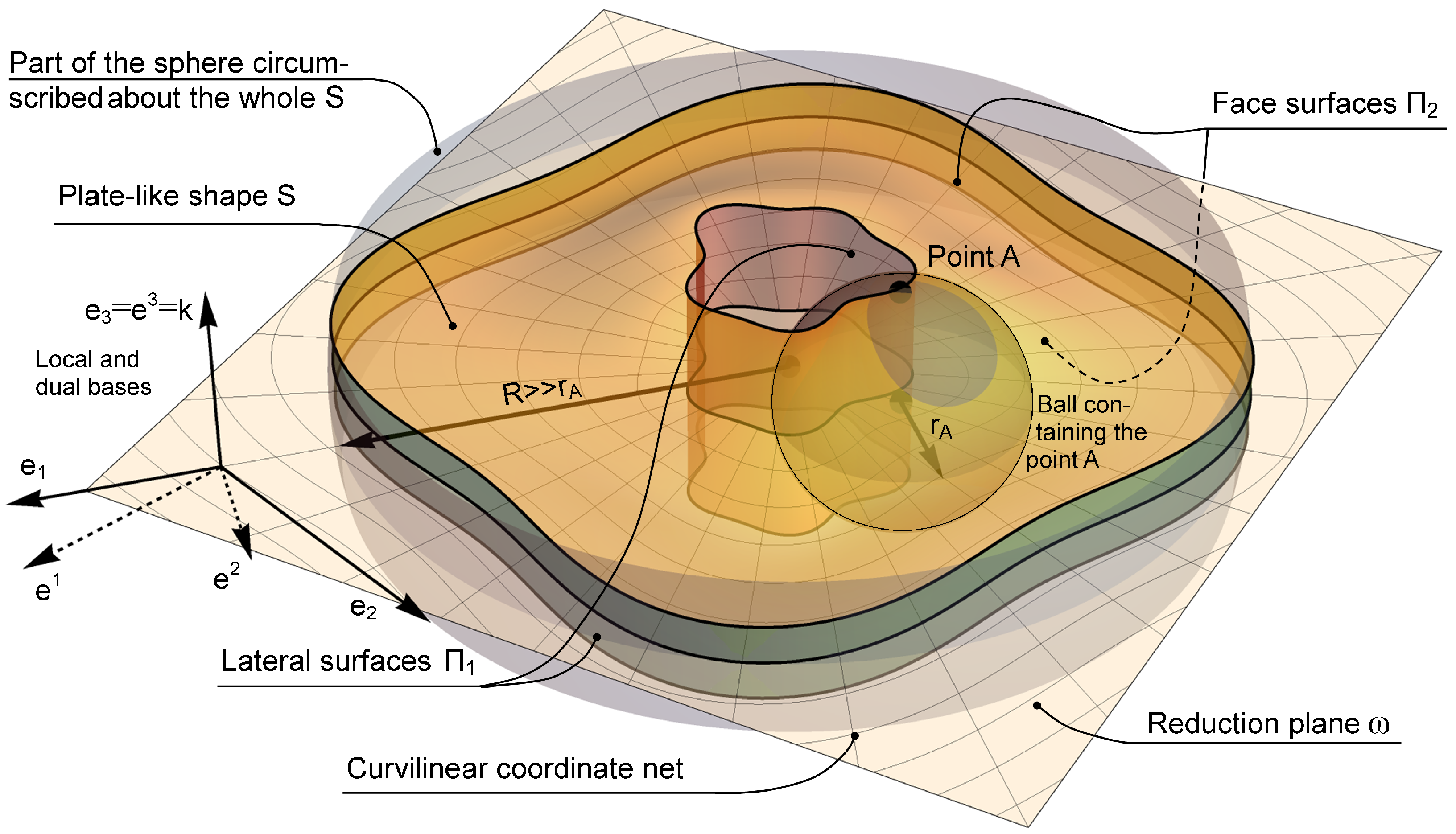
In the paper we will use the concept of a plate-like shape, which can be formalized as a shape , whose boundary can be decomposed into two parts:
and meets the following conditions: (i) There exists a plane such that for each point A on there is a ball containing this point, whose center lies on ; (ii) The radius of this ball is much less than the radius R of the sphere circumscribed about the whole (Figure 1). We will refer to as plane of reduction, to connected parts of as face surfaces, and to connected parts of as lateral surfaces. The intersection of the reduction plane and lateral surfaces, i.e., , defines the contour of the plate-like shape.
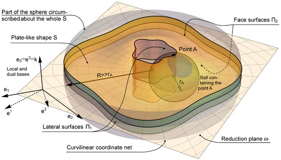
Figure 1.
The geometry of the plate-like shape.
Suppose that a certain shape can be considered the reference shape. Let be the right orthonormal (Cartesian) frame in E such that are parallel to the reduction plane . Thus, at least part can be covered with appropriate curvilinear coordinates as follows:
Hereinafter, symbols , , denote Cartesian coordinates, related with the chosen frame in E.
For simplicity, we will assume that the contour lies entirely in , and connected subsets of are surfaces without self-intersections. Consequently, the shape , as a region in E, can be defined in a coordinate manner by the following extension of the chart onto the neighborhood of :
In the region , which is an open subset of the reduction plane (i.e., subspace of E, spanned over ), one can define the field of frames with a local (oblique in general) basis as follows:
Reciprocal bases can be obtained as solutions of linear inhomogeneous equations . The field of frames and its dual can be expanded on with bases and . Therefore, the defined frames allow us to determine plane and spatial Hamiltonian operators in and correspondingly as follows:
Note that hereinafter we follow [10], defining a gradient operator as the transpose of the formal dyadic product of the appropriate Hamiltonian operator and a field , whose gradient is sought, i.e., . For the sake of brevity, we denote as (without the dyadic product sign). Therefore, and, consequently, if is a vector field, then:
where are Christoffel symbols, related with curvilinear coordinates on .
We define deformation as a diffeomorphism [41] that maps the region onto region , i.e.,
This map induces deformation of the reduction plane as the restriction of to :
Here, denotes the image of the reduction plane, , which can be referred to as the reduction surface.
Because both sets and are regular regions in , they inherit an affine-Euclidean structure, which makes it possible to define the vector field of displacements:
Recall now that the reference shape is plate-like, so we can take advantage of expansion over a small parameter, related with the thickness of the plate. To this end, we consider the displacement field (1) as power expansion
with coefficients, which can be (under well-known analytical assumptions) derived directly as derivatives of :
Thus, instead of a 3D problem with respect to , one can consider a 2D problem with respect to the sequence of unknowns , which is much simpler than the former. In this instance, the deformation gradient can be evaluated in terms of :
With only a finite number of items, we arrive at the asymptotic representation. If we take into account items whose degrees are not higher than one, then, formally:
The appearance of in the expression for the deformation gradient is asymptotically consistent, but leads to a discrepancy with the conventional approach in shell theory. To avoid this discrepancy, we can either neglect this term, or change the approach to the deformation, considering (2) as an exact expression for 2D Cosserat continuum deformation. In present paper, we take the latter approach and rewrite formulae (2) as follows:
and consider the displacements (in accordance with the Euler–Chasles theorem) as a composition of displacements of points in and rotations of line elements, which are transversal to , i.e.,
where is a proper orthogonal tensor (, ). For small values of the approximation , where is an asymmetric tensor, is valid, so we arrive at the Uflyand–Mindlin representation for displacements.
3. Classical Formulation
For the modeling of the elastic plate response, we use the least action principle and variational symmetries. With this approach, the field equations and natural boundary conditions can be derived from the stationary-action condition, while the conservation laws follow from the invariance of the action with respect to coordinate and field variations. Thus, the main attention should be paid to the formulation of the action functional, while everything else may be obtained with formal derivation. This approach is useful for the analysis of elastic systems with additional degrees of freedom, whose geometric interpretation may not be so obvious, such as generalized models of plates and shells. At the same time, this formal derivation can lead to cumbersome equations with unclear geometric meaning, and when using it, it is useful to make comparisons with similar models derived within the conventional 3D elasticity. With this in mind, we first analyze the variational formulation for the plate-like solid, regarding it as a 3D simple isotropic hyperelastic body. Along the way, we stipulate conditions on the material properties, which we assume in both 3D and 2D formulations. These are as follows:
- The material is hyperelastic, i.e., a stored-energy function exists and does not depend on the deformation history.
- The material is simple, i.e., the values of the stored-energy function at a point depend only on deformation within the infinitesimal neighborhood of the point.
Under these assumptions one can formulate the action functional as an iterated integral over the time interval and the region in physical space, which coincides with the reference shape of a plate-like solid:
Here denote the instants of starting and finishing the deformation process, is the density of the action (Lagrangian) which, according to the assumptions above, depends on position vector , current instant t, and the first derivatives over the spatial and time variables (the dot denotes the time derivative). The last item in the integrand stands for the Jacobian, which is the square root of the determinant of the metric form, related with adopted curvilinear coordinates:
The standard reasoning carried out within the framework of the Lagrangian formalism assumes separate transformations for the spatial and time derivatives, which makes the derivation of the field equations and conservation laws rather cumbersome. To avoid this cumbersomeness, we propose the use of a (3+1)D formulation, which allows us to derive the equations in a more concise form. To this end, we introduce the (3+1)D event vector and the (3+1)D nabla operator:
where is a formal unit vector, orthogonal to all elements of the local spatial basis (one can regard as the basis in direct sum ).
Remark 1.
(3+1)D representations make it possible to combine differentiation with respect to spatial variables and time within one differential operation . However, we do not use the specifics of the four-dimensional frame decomposition on a time-like line and spatial platform with respect to the observer, adopted in the special theory of relativity [44], since we assume the velocities of material points to be sufficiently small. Therefore, we suppose that such decomposition is fixed and (3+1)D Minkowski space has a trivial global structure of the direct sum . In this regard, one can identify a (3+1)D space with Galilean space-time.
Within this formalism, action (3) for (3+1)D event (4) and displacements (1) can be written as follows:
where
is the (3+1)D representation for the Lagrangian, adopted in (3), is the projector onto , denotes the identity over , while , is a (3+1)D cylindrical region (world-tube of the shape ), and denotes a (3+1)D volume element in coordinate space that is simply the product of the spatial and time increments: . The use of such an elementary volume implies that the Jacobian, related with the curvilinear coordinates used, is accounted for within .
One can define a (3+1)D metric tensor in as . The negative sign in front of the time-like unit vector is needed only so that d’Alembert-type operators can be represented in the simplest form in terms of four-divergences. Then, the Lagrangian will be supplied with metric multiplier instead of . This notation is commonly used in relativity, but for brevity we will not explicitly indicate this in the notation in this paper. At the same time, one should keep in mind the (3+1)D metric for a correct understanding of the scalar product, denoted with . Although the dot product symbols in 3D and (3+1)D are typographically indistinguishable, the difference is always clear from the context.
Within conventional non-linear elasticity, the density of the action, i.e., Lagrangian, can be split into three items:
The first item, , defines kinetic energy; the second, , determines stored elastic energy; and the last, , denotes the work done by external fields.
In accordance with the constraints adopted in classical continuum mechanics, the expression for the stored elastic energy must satisfy the principle of material indifference [10]:
Here, is an arbitrary proper orthogonal tensor in , i.e., , ( denotes the identity in ). Thus, the stored elastic energy has to be defined as the following composition
where stands for the symmetrizing operator, i.e., for arbitrary second-rank tensor this operator
returns the self-conjugate (symmetric) part of . Writing the deformation gradient in the form of Cauchy polar decomposition, , , where is symmetric, i.e., , and is proper orthogonal, i.e., , we arrive at a specific form for functional , which depends on the right Cauchy–Green strain tensor :
To define a particular form of functional , it is necessary to account for stretches relative to some uniform (for example, stress-free) state. Generally, solids cannot be transformed entirely into uniform states due to incompatible deformations and residual stresses occurring in them. These factors turn out to be especially important in micron-scale elastic bodies, particularly in the elements of MEMS structures. The key concepts of incompatible deformation theory are described in [45,46]. The basic idea is that the uniform state can be achieved only locally by local deformation , which in general does not meet any compatibility conditions, i.e., . Consequently, the whole solid cannot be represented as a gradient of some vector field and this is the main difference from the conventional deformation gradient . To take such local deformations into account, one has to rewrite the functional in the form:
related with total distortion:
Note that even in the case when does not explicitly depend on and is an isotropic function with respect to the second argument (which corresponds to a homogeneous and isotropic material), depends on via and remains an isotropic function only for particular values of . Thus, a locally homogeneous and isotropic material turns out to be inhomogeneous and anisotropic as part of a self-stressed body. This fact is characterized by the concepts of material uniformity and inhomogeneity [47,48,49,50].
Further reasoning is grounded on the the least action principle
A feature of the variational approach used below is that the variation of the functional is calculated with respect to the total variation of coordinates and fields [47,51]. In doing so, we firstly define families for coordinates , and fields , which depend on scalar parameter such that
Then, the total variation can be defined as follows:
where denotes an arbitrary sufficiently small increment of the parameter . These variations cause variations in the action functional, which, after obvious transformations involving the chain rule and Stokes theorem, can be represented in the following equivalent forms:
Here, denotes the total variation of the Noether current, stands for the Euler–Lagrange differential expression and denotes the energy-momentum tensor
while denotes the Lagrangian explicit gradient, i.e.,
The detailed derivation of the above formulae can be found in [52] (one needs to keep in mind that in the paper [52], Gibbs notation is used for the nabla operator).
From partial variations, in which the fields vary while the coordinates remain fixed, we follow field equations and natural boundary conditions:
Another type of partial variation, with fixed fields and varying coordinates, gives conservation laws as follows:
According to Noether theorem, specific forms of conservation laws can be derived from general relation (7) if a particular group of variations (translations and rotations) is specified. Corresponding conservation laws are given in Table 1. The “strong” column shows the conservation laws that hold regardless of the field Equation (6). The column “weak” contains the conservation laws provided that the field equations are satisfied. In the table, is an arbitrary vector in (3+1)D, guiding the translation; denotes finite rotations about an arbitrary axis in (3+1)D; is a corresponding antisymmetric tensor that represents infinitesimal rotations; and denotes the energy momentum – momentum tensor, .

Table 1.
Conservation laws for 3+1D formulation.
Even though the (3+1)D formulation leads to concise equations, it is useful to show at least once their transformation to the conventional form. For field equations and boundary conditions (6) this transformation has the form:
where is the lateral part of (3+1)D volume , instants , define corresponding bases of this volume, denotes Piola stresses, stands for linear momentum and is the volume force:
All these fields are related with the (3+1)D fields as follows:
Obviously, , and along with the Piola stresses one can derive the Cauchy stresses with the Piola transformation . Of course, the right-hand sides in the boundary conditions (8) may be inhomogeneous. In this case, they can be converted to homogeneous conditions using a standardization procedure. A more drastic difference between this formulation of the boundary-value problem and the classical one is that the time-like boundary conditions are specified for the initial and final instants, instead of the field values and their time derivatives in the initial instant only. Meanwhile, this feature is characteristic of the Lagrangian approach and it is possible to obtain the usual conditions for functions and their derivatives at the initial instant only by fundamentally changing the structure of the action functional; for example, by constructing it on the basis of the convolutive principle. Here, we will not do this and reconcile ourselves with some differences in the formulation of the initial-boundary value problem.
A more complex object that contains information about incompatible deformations in energetic format is the energy-momentum tensor . It can be decomposed as follows:
where is the Eshelby stress tensor, denotes the canonical momentum, is the Hamiltonian density and stands for the Umov–Poynting vector:
The conservation law for the energy-momentum tensor, which can be rewritten as a balance law with a non-zero RHS, results in balance equations for canonical momentum and energy flux:
Here, denotes configurational force, while stands for dissipative force:
We emphasize that it is the configurational and dissipative forces that determine the nontrivial self-stress state caused by incompatible deformations and their evolution. Indeed, these forces arise due to spatial and temporal inhomogeneity, which, in turn, arise due to the inhomogeneous field of the implant and its evolution in time. In this case, surface effects can be represented by some special distribution of the implant field on the front surfaces of the plate, which formally leads to the same mathematical formalism.
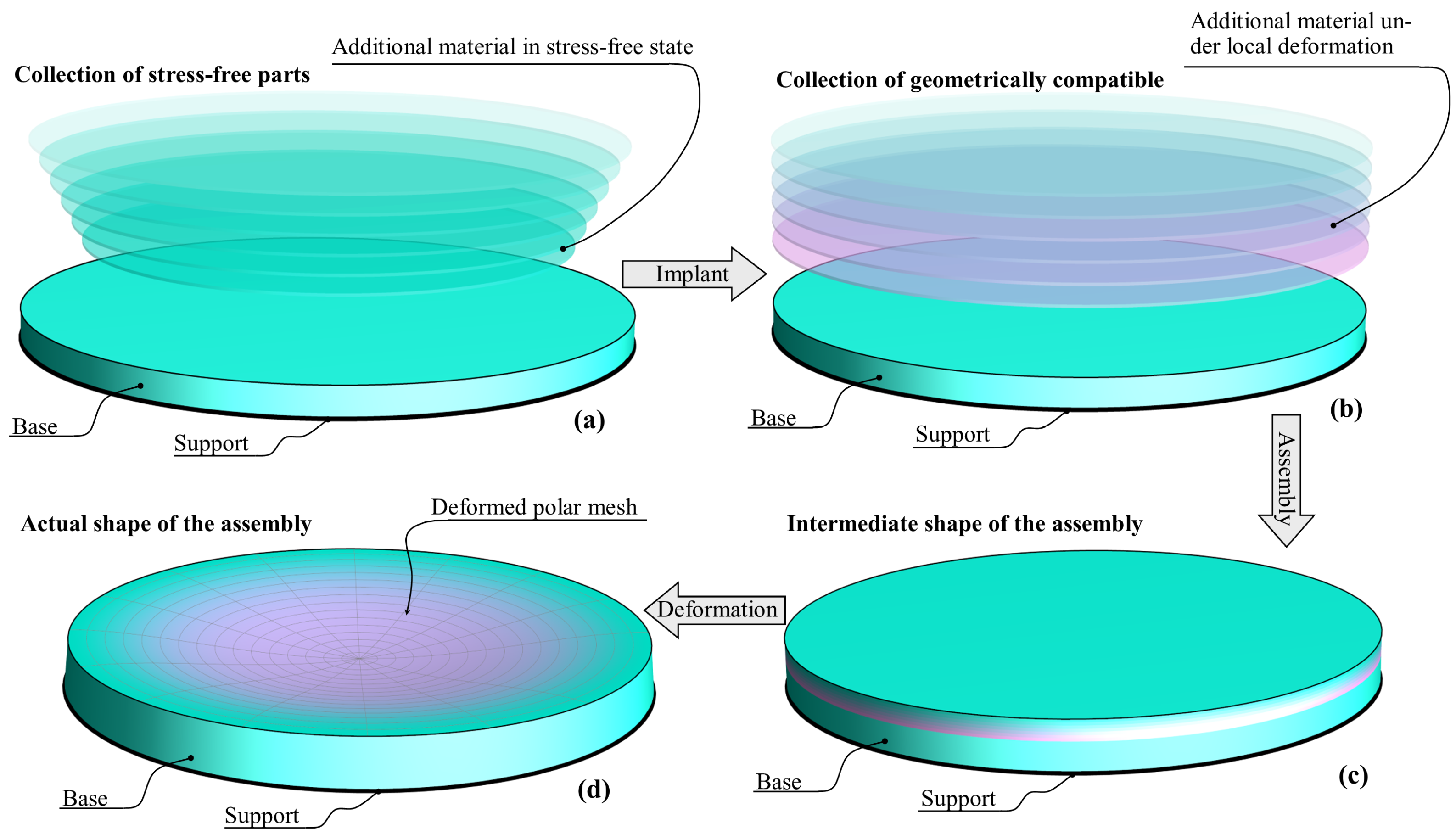
To illustrate the obtained relations, consider the model problem for a self-stressed hyperelastic circular plate (Figure 2). The displacements of the plate are constrained in the transversal (vertical) direction along the circular support that is shown in Figure 2 by a black thick line. The plate can be brought into a stress-free state by being divided into disjointed parts (Figure 2a). As a result of assembling these parts, all of which have been subjected to local deformation, a certain self-stressed shape can be obtained. Of all the possible shapes, it is advisable to choose the shape with the simplest geometry as a reference shape (Figure 2b). This shape is in equilibrium only under the action of specific volume forces that balance it (Figure 2c). In the absence of external fields, the entire assembly is deformed into some distorted shape (Figure 2d).
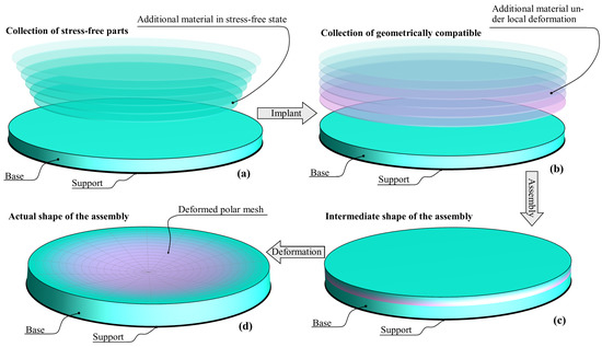
Figure 2.
Model problem for a self-stressed hyperelastic circular plate: (a) The plate with the collection of stress-free additional layers. (b) The local deformation of additional layers that provides geometric compatibility. (c) The assembly that is balanced by a specific field of volume forces. (d) The distorted shape of the assembly in the absence of external fields.
To provide a more comprehensive description of the stressed state, we assume that the elastic potential is of the Saint-Venant–Kirchhoff type, i.e.,
where , are material constants that correspond to Lamé elastic moduli in the linear approach, and denotes Green–Saint-Venant strain. Here, of course, we understand the stress tensor in the local sense. This potential corresponds to the constitutive equation, which expresses the second Piola–Kirchhoff stress tensor with as follows:
Note that we specifically chose a potential that gives a constitutive equation close in form to Hooke’s law. At the same time, these relations are more general than their counterparts in the linear approach.
To illustrate the effects caused by incompatible local deformations, it is enough to set them in the form of some law, without relating it to a specific technological process. For simplicity, we assume that the implant (tensor inverse to local deformations of a geometrically incompatible part of the assembly) is spherical and linearly depends on the transversal coordinate:
where a, b are some constants (we will refer to a particular value of multiplier as the implant factor). Thus, we consider a certain model assembly process, during which infinitely thin stretched layers are attached to the substrate, the measurement of stretching of which changes during the process. This process generally corresponds to the technology of layer-by-layer deposition, during which the implant factor changes due to changes in the temperature field and the evolution of incompatible thermomechanical deformations. Of course, for a more detailed description, the law of change in the implant field should not be specified, but found from the solution of the evolutionary problem. However, a discussion of these issues is beyond the scope of this article. We only mention that evolutionary problems are described in more detail in [36,45,53].
Computational modeling was performed using the finite element method with the following data:
- Elastic moduli (silicon) GPa, GPa;
- Diameter of the plate 1 mm;
- Initial thickness of the plate mm;
- Final thickness of the plate mm;
- Initial implant factor ;
- Final implant factor 0.
The results of the computer simulation are given in Figure 3. The figure shows a diagram that compares the dependences of the thickness of the assembly and the implant factor of the upper layer depending on the time-like variable (Figure 3a). For three moments corresponding to 10%, 50% and 100% of the assembly process, the distributions of the von Mises stress intensity (Figure 3b) and stored elastic energy (Figure 3c) are given. Note that non-zero distributions of stored energy in the absence of external force fields precisely characterize the inhomogeneity caused by incompatible deformations. By differentiating with respect to the spatial variables, one can find configurational force , and by differentiating with respect to a time-like variable, one can find the dissipative force (9). The latter characterizes that part of the mechanical work that was performed during the assembly of the intermediate shape, but was not returned when this shape was deformed into the actual one. Accounting of elastic energy irretrievably stored in the body during the process of its creation is a key factor in understanding the deformation peculiarities of ultrathin plates [4].
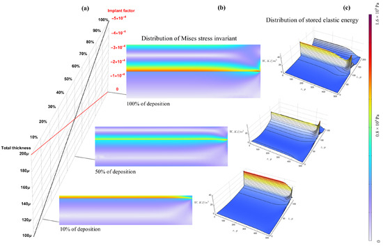
Figure 3.
Results of computer simulation: (a) Changing of the assembly thickness and the implant factor of the upper layer during the deposition process. (b) Distribution of the von Mises stress intensity. (c) Distribution of the stored elastic energy.
4. Micropolar Formulation
Imagine now that instead of a 3D body, we observe only the surface of reduction , which is a part of the plane, embedded in (generally it does not necessarily lie inside the reference shape ). All we can observe is the bending and stretching of this surface. The stretching is characterized by 2D deformations, similar to those in 3D, only when one spatial dimension is ignored. However, the bending, i.e., the changes in the curvature and transversal displacements, has to be characterized in a fundamentally new way. From the various methods, we choose the Cosserat approach [10,54,55,56]. This approach allows extra degrees of freedom to be taken into account, which may be interpreted either as internal deformations, for example, micro-deformations of individual grains in a polycrystalline solid, or external deformations, related with bending, that cannot be directly observed within the 2D geometry of the reduction surface [10,19,56,57].
Within this approach, the action is defined on and can be written as follows
Here, denotes the density of action with respect to area element , stands for a tuple of surface coordinates for a material points on and is a second-rank tensor field that describes local extra deformation of a specific kind. It can be interpreted as a linear transformation of hidden geometric parameters associated with an elementary volume, which, in turn, is identified by the material point of the deformed body. Within the general Cosserat approach, the components of are considered to be independent from each other and do not depend on conventional deformations, represented by the field . In such cases, are referred to as micromorphic deformations [54] and can be represented by means of a set of vectors , (possibly not related in any way to translational vectors from ), referred to as directors: . Generally, the directors can be defined in some abstract vector space with dimension n, differing from 2 and 3. Meanwhile, for the modeling of plate and shell deformations within the framework of the conventional approach, such a generality is redundant, since the additional degrees of freedom are associated with rotations of a normal element, i.e., a material fiber that is oriented transversal to the surface of reduction in the reference shape. This means that the tensor field acts in (so ) and its components are coupled by the orthogonality relation . Thus, the components of cannot be considered as independent functions, and in order to apply the variational technique, it is important to express them via independent functions. We can obtain such an expression with Rodrigues’ formula:
where is a vector field whose components do not relate to each other. Geometrically, the vector can be expressed with unit vector that defines the axis of rotation and the angle of rotation as follows: . Straightforward calculations show that
where denotes the vectorial invariant (Gibbs cross) of the tensor .
For a 3D solid, we will use space-time formalism in order to obtain equations in concise form and represent the action as:
Here, is the (2+1)D cylindrical space-time domain with base , while denotes the action density with respect to (2+1)D space-time coordinate volume , i.e.,
and is a (2+1)D event vector, whose first component is time-like and whose last two components are space-like. The symbol denotes the 3D space-time nabla operator:
In the above formula is the projector onto , and denotes the identity over . Symbol g stands for the determinant of the metric tensor defined on . Generally, we should distinguish this from the metric determinant in (3). Meanwhile, because of the specific form of the decomposition (3), their numerical values coincide, so we will not use different designations for them.
Repeating the reasoning given above for the 3D solid, we believe that the Lagrangian can be represented as the following splitting:
where is the kinetic energy density, determines the stored elastic energy density and defines the specific work exerted by external fields. Obviously, all densities are defined in relation to the area element .
For 3D solids, we adopt the principle of material frame-indifference. Thus, the functional shall satisfy the condition
where is an arbitrary proper orthogonal tensor in . Note that, despite the fact that the density of stored elastic energy is determined on the 2D plane , the orthogonal tensor is defined in the ambient 3D physical space. Furthermore, the orthogonal transformations that act on the conventional deformation gradient and orthogonal transformations of microdeformations are carried out in a consistent manner, by means of the same tensor . Note this difference between the Cosserat shell theory and the abstract theory for a micromorphic continuum, within which the transformation of microdeformation , associated with a material point, is independent of the transformation of the affine space containing the point.
The condition (11) will be satisfied if one defines in a particular form, replacing the arguments , , with their combinations, which are invariant under the 3D transformation (5). Since itself defines the orthogonal transformation , hence, does not explicitly depend on . Two other arguments may be taken as , . These combinations are invariant with respect to and in the linear approximation correspond to conventional kinematic hypotheses of the classical linear theory of shells. To eliminate the mutual dependence between the components of these fields (arising in view of the orthogonality of ), following [56,57], we introduce strain measures and via the relations
From the last relation, one can explicitly express as
Here, denotes the Levi–Civita tensor.
Consequently, the arguments of functional can be specified as follows:
To take local incompatible deformations into account, one can define the functional with respect to the uniform state as
where is the local 2D deformation (generally incompatible), similar to the one defined above for the 3D solid; is the local orthogonal transformation that brings the directors into a uniform state.
With (10), (14) and (15), one can consider the Lagrangian either as an explicit function on , , or as the following compositions:
The explicit form via gives the field equations and conservation laws in the most simple form that reflects only the first-order character of the theory and the structure of the collection of fields. The forms with compositions , and result in the field equations, stress resultants, and boundary conditions like those used in conventional shell theory. The last form, written in terms of , , , , and makes it possible to use in the Lagrangian an expression for elastic energy coinciding with the standard expression, which is usually measured in mechanical tests on standard samples deformed from a uniform state. It is that represents the initial information about the physical and mechanical properties of the material, which can be obtained as a result of testing standard samples. However, represents an explicit dependence on kinematic functions for a self-stressed body whose inhomogeneity and anisotropy are induced by incompatible deformations of its constituent elementary volumes.
Assuming that the Lagrangian depends on coordinates and fields , , whose components do not depend each on other, we arrive at the expression for variation of the action in the following equivalent forms:
Here, the variation of the Noether current, , Euler–Lagrange equations, , , and Eshelby stress tensor, , take the forms:
while denotes the Lagrangian explicit gradient with account of the microrotation fields:
As above, from partial variations, in which the fields vary while the coordinates remain fixed, we have the following field equations:
and natural boundary conditions:
The partial variations with fixed fields and varying coordinates give the conservation laws in Table 2; denotes an arbitrary vector in (2+1)D, whose spatial part belongs to ; stands for arbitrary rotations also in (2+1)D (spatial rotations are exhausted by rotations about axis ); is an asymmetric tensor that is an infinitesimal counterpart of ; and is a (2+1)D energy momentum-momentum tensor.
Table 2.
Conservation laws for (2+1)D formulation.
The field Equation (16) can be transformed to a more familiar form if the stored elastic energy functional is presented as an explicit dependence on strain measures (12) and (13). In this case, taking into account the expressions for partial variations of strain measures:
where for brevity the following notation is used:
and, consequently, for the density of stored elastic energy:
we arrive at field equations in the following well-recognizable form:
Here,
are conventional quantities related with stress and momentum resultants.
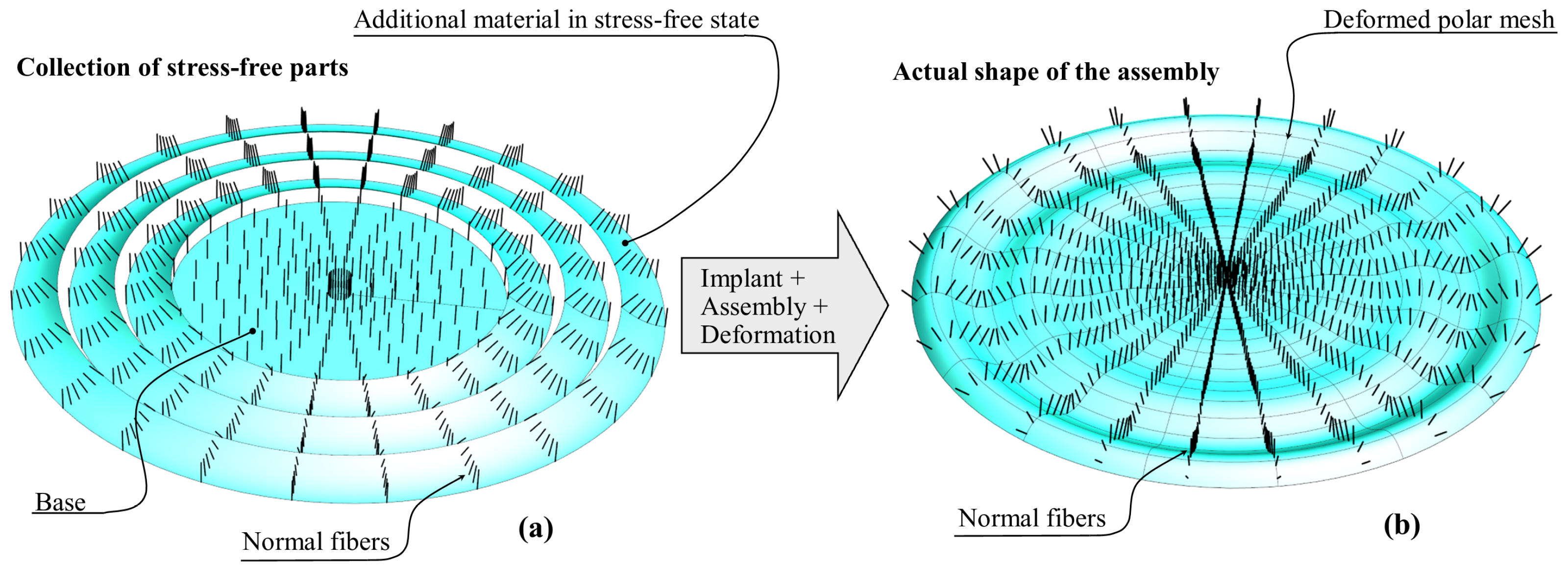
An illustration similar to that shown in Figure 2, but adapted to the case of the Cosserat continuum and two implant fields, is shown in Figure 4. For brevity, it skips the stages of assembling the intermediate shape, but along with the geometric images of the shape, the fields of the directors are shown, whose roles are played by the fibers (normal elements) of the plate. Figuratively speaking, to assemble a collection of geometrically incompatible Cosserat-like shapes, it is necessary not only to coordinate the geometric regions they occupy, but also the orientation of their fibers. This fact clearly highlights the need for two implant fields.
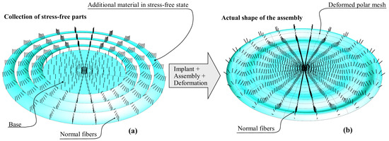
Figure 4.
The assembly of Cosserat-type shapes: (a) The plate with the collection of stress-free additional layers. (b) The distorted shape of the assembly.
5. Conclusions
We draw conclusions on the work in the following theses:
- Formalization of incompatible deformations through the implant field provides an effective mathematical formalism for residual stress modeling.
- When modeling incompatible deformations within the framework of Cosserat’s theory, it is necessary to take into account two types of implants associated with local translations and local rotations.
- The account of incompatible deformations as sources of residual stresses makes it possible to theoretically explain a significant increase in the rigidity of ultrathin MEMS elements.
Author Contributions
Conceptualization and methodology, S.L.; writing—original draft preparation, S.L., A.D., V.B. and N.D. All authors have read and agreed to the published version of the manuscript.
Funding
This research was supported by the Ministry of Science and Higher Education of the Russian Federation under contract No. 075-15-2021-1350, dated 5 October 2021 (internal number 15.SIN.21.0004).
Institutional Review Board Statement
Not applicable.
Informed Consent Statement
Not applicable.
Data Availability Statement
The study does not report any data.
Acknowledgments
We wish to say that in working on the paper we have had the assistance of our colleague K. Koifman, and that we are indebted to him for several valuable suggestions.
Conflicts of Interest
The authors declare no conflicts of interest.
Abbreviations
The following abbreviations are used in this manuscript:
| MEMS | Microelectromechanical systems |
| RHS | Right-hand side |
Some designations used
| Deformation gradient | Action | ||
| Right stretch tensor | Four Lagrangian | ||
| Cauchy–Green strain tensor | Noether current | ||
| Green–Sen-Venant strain tensor | Euler – Lagrange operator | ||
| Metric deformation measure | Energy-momentum tensor | ||
| Bending deformation measure | Energy momentum – momentum tensor | ||
| Local deformation field | Linear momentum | ||
| Local orthogonal transformation | Eshelby stress tensor | ||
| First Piola stress tensor | Canonocal momentum | ||
| Second Piola stress tensor | Hamiltonian density | ||
| Cauchy stress tensor | Umov–Poynting vector |
References
- De Teresa, J.M. Nanofabrication: Nanolithography Techniques and Their Applications; IOP Publishing: Bristol, UK, 2020. [Google Scholar]
- Bhushan, B. Mechanical Properties of Nanostructures. In Springer Handbook of Nanotechnology; Bhushan, B., Ed.; Springer: Berlin/Heidelberg, Germany, 2004. [Google Scholar]
- Corigliano, A.; Ardito, R.; Comi, C.; Frangi, A.; Ghisi, A.; Mariani, S. Mechanics of Microsystems; John Wiley & Sons: Hoboken, NJ, USA, 2018. [Google Scholar]
- Lychev, S.A.; Digilov, A.V.; Demin, G.D.; Gusev, E.E.; Kushnarev, I.V.; Djuzhev, N.A.; Bespalov, V.A. Deformations of Single-Crystal Silicon Circular Plate: Theory and Experiment. Symmetry 2024, 16, 137. [Google Scholar] [CrossRef]
- Eremeyev, V.A.; Altenbach, H.; Morozov, N.F. The influence of surface tension on the effective stiffness of nanosize plates. Dokl. Phys. 2009, 54, 618–621. [Google Scholar] [CrossRef]
- Eremeyev, V.A. On effective properties of materials at the nano- and microscales considering surface effects. Acta Mech. 2016, 227, 29–42. [Google Scholar] [CrossRef]
- Dedkova, A.A.; Glagolev, P.Y.; Gusev, E.E.; Djuzhev, N.A.; Kireev, V.Y.; Lychev, S.A.; Tovarnov, D.A. Peculiarities of deformation of round thin-film membranes and experimental determination of their effective characteristics. Tech. Phys. 2021, 91, 1454–1465. [Google Scholar] [CrossRef]
- Timoshenko, S.P.; Woinowsky-Krieger, S. Theory of Plates and Shells; McGraw-Hill: New York, NY, USA, 1959. [Google Scholar]
- Lebedev, L.P.; Cloud, M.J.; Eremeyev, V.A. Tensor Analysis with Applications in Mechanics; World Scientific: Hackensack, NJ, USA, 2010. [Google Scholar]
- Truesdell, C.; Noll, W. The Non-Linear Field Theories of Mechanics; Springer: Berlin/Heidelberg, Germany, 2004. [Google Scholar]
- Reddy, J.N. Theory and Analysis of Elastic Plates and Shells; Taylor & Francis: Philadelphia, PA, USA, 2007. [Google Scholar]
- Zubov, L.M. Non-Linear Elasticity Theory Methods in the Shells Theory; Izd-vo Rostovskogo Universiteta: Rostov-on-Don, Russia, 1982. (In Russian) [Google Scholar]
- Pietraszkiewicz, W. Geometrically nonlinear theories of thin elastic shells. Adv. Mech. 1989, 12, 51–130. [Google Scholar]
- Eremeyev, V.A.; Pietraszkiewicz, W. The nonlinear theory of elastic shells with phase transitions. J. Elast. 2004, 74, 67–86. [Google Scholar] [CrossRef]
- Euler, L. De motu vibratorio tympanorum. Novi Comment. Acad. Sci. Petropolitanae 1766, 10, 243–260. (In Latin) [Google Scholar]
- Euler, L. Tentamen de sono campanarum. Novi Comment. Acad. Sci. Petropolitanae 1766, 10, 261–281. (In Latin) [Google Scholar]
- Kirchhoff, G. Über das Gleichgewicht und die Bewegung einer elastischen Scheibe. J. Reine Angew. Math. (Crelles J.) 1850, 40, 51–88. (In German) [Google Scholar]
- Ufly, Y.S. Wave Propagation by Transverse Vibrations of Beams and Plates. J. Appl. Math. Mech. 1948, 12, 287–300. (In Russian) [Google Scholar]
- Mindlin, R.D. Influence of rotatory inertia and shear on flexural motions of isotropic, elastic plates. J. Appl. Mech. 1951, 18, 31–38. [Google Scholar] [CrossRef]
- Kil’chevskiy, N.A. Fundamentals of the Analytical Mechanics of Shells; NASA TT, F-292; NASA: Washington, DC, USA, 1965.
- Grigoluk, E.I.; Selesov, I.T. Non-classic Theories of the Vibrations of Rods, Plates and Shells. In Solid mechanics; VINITI: Moscow, Russia, 1973; Volume 5. (In Russian) [Google Scholar]
- Cauchy, A.L. Sur l’equilibre et le mouvement d’une plaque solide. Exerc. Mat. 1828, 3, 328–355. (In French) [Google Scholar]
- Poisson, S.D. Mémoire sur l’équilibre et le mouvement des corps élastiques. Mém. l’Acad. Sci. l’Inst. Fr. 1829, 8, 357–570. (In French) [Google Scholar]
- Lauricella, G. Equilibrio dei corpi elastici isotropi. Ann. Sc. Norm. Super. Pisa 1895, 7, 1–120. (In Italian) [Google Scholar] [CrossRef]
- Vekua, I.N. Shell Theory, General Methods of Construction; Pitman Advanced Publishing Program: Boston, MA, USA, 1985. [Google Scholar]
- Lechnitsky, S.G. Anisotropic Plates; Gostechizdat: Moscow, Russia, 1947. (In Russian) [Google Scholar]
- Föppl, A. Vorlesungen über technische Mechanik. In Vorlesungen Über Technische Mechanik; Föppl, A., Ed.; B. G. Teubner Verlag: Leipzig, Germany, 1907; Volume 5. (In German) [Google Scholar]
- Kármán, T. Festigkeitsprobleme im Maschinenbau. In Encyclopadie der Mathematischen Wissenschaften; Klein, F., Muller, C., Eds.; B. G. Teubner Verlag: Leipzig, Germany, 1910; Volume 4. (In German) [Google Scholar]
- Vol’mir, A.S. A Translation of Flexible Plates and Shells; Air Force Flight Dynamics Laboratory, Research and Technology Division, Air Force Systems Command: Ohio, OH, USA, 1967. [Google Scholar]
- Ciarlet, P.G. A justification of the von Kármán equations. Arch. Ration. Mech. Anal. 1980, 73, 349–389. [Google Scholar] [CrossRef]
- Yang, W.H.; Feng, W.W. On axisymmetrical deformations of nonlinear membranes. J. Appl. Mech. 1970, 37, 1002–1011. [Google Scholar] [CrossRef]
- Green, A.E.; Adkins, J.E. Large Elastic Deformations and Non-Linear Continuum Mechanics; Clarendon Press: Oxford, UK, 1960. [Google Scholar]
- Rivlin, R.S.; Thomas, A.G. Large Elastic Deformations of Isotropic Material VIII. Strain Distribution Around a Hole in a Sheet. Philos. Trans. R. Soc. 1951, 243, 289–298. [Google Scholar]
- Adkins, J.E.; Rivlin, R.S. Large Elastic Deformations of Isotropic Material IX. The Deformations of Thin Shells. Philos. Trans. R. Soc. 1952, 244, 505–531. [Google Scholar]
- Klingbeil, W.W.; Shield, R.T. Some Numerical Investigations on Empirical Strain-Energy Functions in the Large Axi-symmetric Extensions of Rubber Membranes. Z. Angew. Math. Phys. 1964, 15, 608–629. [Google Scholar] [CrossRef]
- Lychev, S.A.; Koifman, K.G. Geometry of Incompatible Deformations: Differential Geometry in Continuum Mechanics; De Gruyter: Berlin, Germany, 2018. [Google Scholar]
- Epstein, M.; Elzanowski, M. Material Inhomogeneities and Their Evolution: A Geometric Approach; Springer Science: New York, NY, USA, 2007. [Google Scholar]
- Steinmann, P. Geometrical Foundations of Continuum Mechanics: An Application to First- and Second-Order Elasticity and Elasto-Plasticity; Springer: Berlin/Heidelberg, Germany, 2015. [Google Scholar]
- Rakotomanana, L. A Geometric Approach to Thermomechanics of Dissipating Continua; Birkhäuser: Boston, MA, USA, 2004. [Google Scholar]
- Marsden, J.; Hughes, T. Mathematical Foundations of Elasticity; Courier Corp.: New York, NY, USA, 1994. [Google Scholar]
- Lee, J.M. Smooth Manifolds; Springer: New York, NY, USA, 2012. [Google Scholar]
- Epstein, M. Differential Geometry: Basic Notions and Physical Examples; Springer International Publishing: Cham, Switzerland, 2014. [Google Scholar]
- Kellogg, O.D. On the derivatives of harmonic functions on the boundary. Trans. Am. Math. Soc. 1931, 33, 486–510. [Google Scholar] [CrossRef]
- Gourgoulhon, E. Special Relativity in General Frames; Springer: Berlin/Heidelberg, Germany, 2013. [Google Scholar]
- Lychev, S.A.; Koifman, K.G.; Djuzhev, N.A. Incompatible Deformations in Additively Fabricated Solids: Discrete and Continuous Approaches. Symmetry 2021, 13, 2331. [Google Scholar] [CrossRef]
- Lychev, S.A.; Koifman, K.G. Contorsion of Material Connection in Growing Solids. Lobachevskii J. Math. 2021, 42, 1852–1875. [Google Scholar] [CrossRef]
- Maugin, G.A. Material Inhomogeneities in Elasticity; CRC Press: Boca Raton, FL, USA, 1993. [Google Scholar]
- Noll, W. Materially Uniform Simple Bodies with Inhomogeneities; Springer: Berlin/Heidelberg, Germany, 1974. [Google Scholar]
- de Feraudy, A.; Queguineur, M.; Steigmann, D.J. On the natural shape of a plastically deformed thin sheet. Int. J. Non-Linear Mech. 2014, 67, 378–381. [Google Scholar] [CrossRef]
- Steigmann, D.J. Mechanics of materially uniform thin films. Math. Mech. Solids 2015, 20, 309–326. [Google Scholar] [CrossRef]
- Gelf, I.M.; Fomin, S.V. Calculus of Variations; Prentice-Hall: Englewood Cliffs, NJ, USA, 1963. [Google Scholar]
- Lychev, S.A. On Conservation laws of micromorphic nondissipative thermoelasticity. Vestn. Samara Univ. Nat. Sci. Ser. 2007, 4, 225–262. (In Russian) [Google Scholar]
- Lychev, S.A.; Koifman, K.G. Nonlinear evolutionary problem for a laminated inhomogeneous spherical shell. Acta Mech. 2019, 230, 3989–4020. [Google Scholar] [CrossRef]
- Eringen, A.C. Microcontinuum Field Theories: Foundations and Solids; Springer: New York, NY, USA, 1999. [Google Scholar]
- Steigmann, D.J.; Bîrsan, M.; Shirani, M. Thin shells reinforced by fibers with intrinsic flexural and torsional elasticity. Int. J. Solids Struct. 2023, 285, 112550. [Google Scholar] [CrossRef]
- Altenbach, H.; Eremeyev, V.A.; Lebedev, L.P. Micropolar shells as two-dimensional generalized continua models. In Mechanics of Generalized Continua; Altenbach, H., Eremeyev, V.A., Maugin, G.A., Eds.; Springer: Berlin/Heidelberg, Germany, 2011; pp. 23–55. [Google Scholar]
- Eremeyev, V.A.; Zubov, L.M. Mechanics of Elastic Shells; Nauka: Moscow, Russia, 2008. (In Russian) [Google Scholar]

Disclaimer/Publisher’s Note: The statements, opinions and data contained in all publications are solely those of the individual author(s) and contributor(s) and not of MDPI and/or the editor(s). MDPI and/or the editor(s) disclaim responsibility for any injury to people or property resulting from any ideas, methods, instructions or products referred to in the content. |
© 2024 by the authors. Licensee MDPI, Basel, Switzerland. This article is an open access article distributed under the terms and conditions of the Creative Commons Attribution (CC BY) license (https://creativecommons.org/licenses/by/4.0/).