Intersection Properties of Finite Disk Collections

Abstract

In this article, we study the intersection of a finite collection of disks in Euclidean space by examining spheres of various dimensions and their poles (extreme values with respect to canonical projections) contained within the intersection’s boundary. We derive explicit formulae for computing these extreme values and present two applications. The first application involves computing the smallest common rescaling factor for the radii of the disk system, which brings the system to a single point of intersection. This calculation allows us to compute the generalized Čech filtration, a crucial tool for the topological data analysis of weighted point clouds. The second application focuses on determining the minimal Axis-Aligned Bounding Box (AABB) for the intersection of a finite collection of disks in Euclidean space, addressing a significant problem in computational geometry. We consider that this work aims to contribute to the fields of topological data analysis and computational geometry by providing new tools for analyzing complex geometric structures.

1. Introduction

One of the new techniques developed for the analysis of large clusters of information, known as Big Data, is Topological Data Analysis (TDA). In TDA, simplicial complexes associated with the data are constructed. These structures include the Vietoris–Rips complex, the Čech complex, and the piecewise linear lower star complex, among others. Of special interest to us is the generalized Čech complex structure ([1,2,3,4]). Although the standard Čech complex is formed by intersecting a collection of disks with a fixed radius, the generalized version allows varying radii. This flexibility enables us to highlight specific data points by assigning or weighting them with larger and/or more rapidly expanding balls while de-emphasizing others using smaller and/or slower-growing balls. This approach proves valuable for handling noisy data sets, offering an alternative to discarding data that may not meet a specific significance threshold [5].

Understanding the patterns of intersections and the timing of intersections among a set of disks in ${\mathbb{R}}^d$, each with potentially different radii, is a fundamental problem ([6,7,8,9]). This leads to the exploration of the generalized Čech complex structure, which captures the intersection information of these disks, regardless of their radii. Rescaling the radii by the same factor, we obtain a filtered generalized Čech complex, where the associated simplicial complexes evolve as the scale parameter varies. In particular, in [10], algorithms are provided to calculate the generalized Čech complex in ${\mathbb{R}}^2$, and [11] presents an algorithm to determine the Čech scale for a collection of disks in the plane.

It is worth mentioning that our initial goal in writing this article was to compute the Čech scale of a disk system, generalizing [11], to provide a powerful tool for understanding the shape (i.e., the geometry) of complex data in higher dimensions. Facing the challenge of generalizing the results in [11] beyond Euclidean spaces of dimension 2, we began with computing the Axis-Aligned Bounding Box (AABB) for the intersection of a finite set of disks, seeking a measure for such an intersection to incorporate it into a numerical method with the objective of approximating the Čech scale. However, we soon realized that the problem was more complex than anticipated. To compute the (minimal) AABB, it was necessary to include the key points we refer later to as $e_q$-poles. In retrospect, the key points for solving the problem in dimension 2, as discussed in [11], can be considered to be the poles of 0-dimensional spheres, a specific case of the i-spheres we study in this paper. Once we characterized the intersection of a set of disks (with generally different radii) through such $e_q$-poles, we were able to solve both problems: computing (approximate) the Čech scale and computing the minimal AABB for the intersection of a disk system.

To establish the necessary foundation for our study, Section 2 introduces crucial concepts and notation that will be used throughout the article, and we focus on analyzing the intersection of a disk system in ${\mathbb{R}}^d$. We start by investigating the intersection of two disks in Section 2.1 and then expand our analysis to a system of m disks in Section 2.2. By applying Helly’s Theorem, we prove that it is sufficient to examine the intersection of all subsystems consisting of $d+1$ disks to determine if the system has a nonempty intersection.

In Section 3, we define Vietoris–Rips systems and Čech systems, together with presenting results regarding the Rips scale and the Čech scale, as well as their connections. In Section 3.1, we present an algorithm that can determine whether the intersection of the system is empty or nonempty. This is achieved by exclusively computing the poles of subsystems of disks (or spheres). Finally, in Section 3.2, we introduce the algorithm that computes an approximation to the Čech scale using the numerical bisection method.

Additionally, in Section 4, we incorporate the concept of a minimal Axis-Aligned Bounding Box (AABB) into our methodology ([12,13,14]). An AABB is a rectangular parallelepiped whose faces are perpendicular to the basis vectors. These bounding boxes frequently arise in spatial subdivision problems, such as ray tracing [15] and collision detection [16]. In this paper, we study AABBs to enclose the intersection of a finite collection of disks. This approach proves valuable for discerning whether the collection intersects at a singular point or not. In this section, we also provide an algorithm for constructing the AABB of a disk system.

2. Intersection Properties of Sphere Systems

Throughout this work, we will refer to a d-disk system M, or simply a disk system, as a finite collection of closed disks in ${\mathbb{R}}^d$ with positive and not necessarily equal radii, i.e.,

$$M=\{D_i(c_i;r_i)\subset {\mathbb{R}}^d\mid c_i\in {\mathbb{R}}^d,r_i>0,1\le i\le m<\infty \}.$$

Moreover, in order to study the intersection properties of a disk system M with the approach addressed in Section 3 and Section 4 of this work, we will conduct a study in this section of the intersection properties of the spheres corresponding to the boundaries of each disk in M, which we call a sphere system and denote by $\partial M$,

$$\partial M=\{\partial D_i\subset {\mathbb{R}}^d\mid D_i\in M\},$$

where ∂ denotes the topological boundary operator.

Following the notation in [17], we introduce the following generalization of the sphere.

Definition 1. 

An i-sphere in ${\mathbb{R}}^d$ is the intersection of a sphere with an affine subspace of dimension i.

Of course, the notions of a sphere (as a $(d-1)$-dimensional surface) and a d-sphere in ${\mathbb{R}}^d$ agree. However, an i-sphere in ${\mathbb{R}}^d$ can also be viewed as the intersection of d-spheres. For instance, the intersection of two spheres typically occurs in a hyperplane, forming a $(d-1)$-sphere in ${\mathbb{R}}^d$. When another d-sphere intersects this configuration, the result may be a $(d-1)$-sphere, a $(d-2)$-sphere, a 0-sphere (a single point), or it might even be empty, all within the same hyperplane. For a disk system $M=\left\{D_i(c_i;r_i)\right\}$ composed of m disks, where $\{c_1,\cdots ,c_m\}$ is a set in general position in ${\mathbb{R}}^d$, the maximum dimension of the affine subspace associated with the i-sphere, obtained from the intersection of all the spheres in $\partial M$, is at most $d-m+1$, or equivalently, $i=d-m+1$. This conclusion is drawn from ([17] (Theorem 2.1) and the fact that the affine hull of $\{c_1,\cdots ,c_m\}$ is of dimension $m-1$. Consequently, the following result is proven.

Lemma 1. 

Let $M=\{D_1(c_1;r_1),\dots ,D_m(c_m;r_m)\}$ be disk system such that $\{c_1,\cdots ,c_m\}$ is a set in general position in ${\mathbb{R}}^d$. Then, the possibilities for the set ${\cap }_{D_i\in M}\partial D_i$ are:

1. 

the empty set;

2. 

a single point;

3. 

a $(d-m+1)$-sphere.

Remarkable points in i-spheres that will play a key role in the rest of the article are the poles. Let ${\pi }_i:{\mathbb{R}}^d⟶\mathbb{R}$ be the canonical projection on the i-th factor for $i=1,...,d$, and let $\{e_1,e_2,...,e_d\}$ be the standard basis of ${\mathbb{R}}^d$.

Definition 2. 

Let $e_q$ be the q-th vector of the canonical base of ${\mathbb{R}}^d$. An $e_q$-north (south) pole of an i-sphere S in ${\mathbb{R}}^d$ is a point on S whose projection on the q-th coordinate is maximum (minimum). In other words, $x\in S$ is the $e_q$-north pole if ${\pi }_q\left(y\right)\le {\pi }_q\left(x\right)$ for all $y\in S-\left\{x\right\}$, where ${\pi }_q$ represents the projection onto the q-th coordinate.

We denote the $e_q$-north pole of S by $s_q^{+}$ and the $e_q$-south pole by $s_q^{-}$.

An i-sphere can have a single $e_q$-pole (north or south) or an infinite number of them, which occurs when a normal vector to the affine space containing the i-sphere is aligned with the vector $e_q$. We are interested in finding the $e_q$-poles of $(d-m+1)$-spheres originating from disk systems $M=\{D_1(c_1;r_1),\dots ,D_m(c_m;r_m)\}$, by taking the intersection ${\cap }_{j=1}^m\partial D_j$. Such $(d-m+1)$-spheres will be denoted by $S_M(c;r)$ to emphasize the disk system M, as well as its center and radius.

Lemma 2. 

Let $M=\{D_1,\dots ,D_m\}$ be a d-disk system such that ${\bigcap }_{j=1}^m{D}_j\ne \varnothing$, and let p be a point in ${\bigcap }_{j=1}^m{D}_j$ such that ${\pi }_q\left(p\right)\le {\pi }_q\left(x\right)$ (resp. ${\pi }_q\left(p\right)\ge {\pi }_q\left(x\right)$) for every x in ${\bigcap }_{j=1}^m{D}_j$. Then, there exists an i-sphere $S=\partial D_{j_1}\cap \cdots \cap \partial D_{j_i}$ such that p is in S and p is the $e_q$-south pole (resp. $e_q$-north pole) of S.

Proof. 

Since ${\cap }_{j=1}^m{D}_j\ne \varnothing$, then $\partial \left({\cap }_{j=1}^m{D}_j\right)\ne \varnothing$, $\partial \left({\cap }_{j=1}^m{D}_j\right)\subset {\cap }_{j=1}^m{D}_j$ due to the closedness of the sets $D_j$, for $j=1,\dots ,m$, and $p\in \partial \left({\cap }_{j=1}^m{D}_j\right)$.

On the other hand, since $\partial \left({\cap }_{j=1}^m{D}_j\right)\subset {\cup }_{i=1}^m\partial D_j$, there exist indices $j_1,\dots ,j_i$ such that $p\in \partial D_{j_r}$ for any $r=1,\dots ,i$; let $\mathsf{\Lambda }\left(p\right)=\{j_1,\dots ,j_i\}\subseteq \{1,\dots ,m\}$ be a maximal subset of indices such that $p\in D_j$ if and only if $j\in \mathsf{\Lambda }\left(p\right)$. We claim that $p\in {\cap }_{r=1}^i\partial D_{j_r}$ is the $e_q$-south pole of $S:={\cap }_{r=1}^i\partial D_{j_r}$.

In effect, let $V_p\subset {\mathbb{R}}^d$ be an open neighborhood of p sufficiently small such that:

1.

Every $x\in V_p\cap \partial \left({\cap }_{j=1}^m{D}_j\right)$ has as maximal set of indices a proper subset of $\mathsf{\Lambda }\left(p\right)$,

2.

$S\cap V_p\subset \partial \left({\cap }_{j=1}^m{D}_j\right)$.

The first condition can be guaranteed by the finiteness of the disk system M, and the second condition is a consequence of the maximality of the set $\mathsf{\Lambda }\left(p\right)$. Therefore, ${\pi }_q\left(p\right)\le {\pi }_q\left(x\right)$ for every $x\in S\cap V_p$, which is equivalent to the fact that ${\pi }_q\left(p\right)\le {\pi }_q\left(x\right)$ for every $x\in S$, in the case of i-spheres.    □

2.1. Sphere Systems with Two Spheres

In the following two lemmas, we provide the computations to determine the center, radius, and poles for a $(d-1)$-sphere given by the intersection of two disks in ${\mathbb{R}}^d$.

Lemma 3. 

Let $M=\{D_1(c_1;r_1),D_2(c_2;r_2)\}$ be a disk system with two d-disks such that $\partial D_1\cap \partial D_2$ is a $(d-1)$-sphere $S=S_M(c;r)$ with center c and radius r. Then,

$$c=\frac{1}{2}\left(1+\frac{r_2^2-r_1^2}{\parallel c_2-c_1{\parallel }^2}\right)c_1+\frac{1}{2}\left(1+\frac{r_1^2-r_2^2}{\parallel c_2-c_1{\parallel }^2}\right)c_2$$

and

$$r=\frac{2\sqrt{s(s-\parallel c_2-c_1\parallel )(s-r_1)(s-r_2)}}{\parallel c_2-c_1\parallel },$$

where $s=\frac{1}{2}(\parallel c_2-c_1\parallel +r_1+r_2)$.

Proof. 

Let $\mathsf{\Pi }$ be the hyperplane containing the $(d-1)$-sphere S, which is defined by the equation:

$$\sum _{i=1}^d(k_i-h_i)x_i-\frac{1}{2}\sum _{i=1}^d(k_i^2-h_i^2)=\frac{r_1^2-r_2^2}{2},$$

(1)

where $c_1=(h_1,\dots ,h_d)$ and $c_2=(k_1,\dots ,k_d)$. Then the normal vector of the hyperplane $\mathsf{\Pi }$ is given by $N:=c_2-c_1=(k_1-h_1,\dots ,k_d-h_d)$, and the center c of S is determined by the intersection point of the hyperplane $\mathsf{\Pi }$ with the perpendicular line that passes through the center $c_1$ of $D_1$. This line can be parameterized as $\gamma :t\mapsto c_1+tN=(x_1\left(t\right),\dots ,x_d\left(t\right))$, such that $\gamma \left(0\right)=c_1$ and $\gamma \left(1\right)=c_2$. We can compute the intersection point $c=\gamma \left(t_{*}\right)$ of $\mathsf{\Pi }$ and $\gamma \left(\right[0,1\left]\right)$, for any $t_{*}\in [0,1]$, by substituting it in (1),

$$\sum _{i=1}^d(k_i-h_i)(h_i+t_{*}(k_i-h_i))=\frac{1}{2}\left(\sum _{i=1}^d(k_i^2-h_i^2)+(r_1^2-r_2^2)\right).$$

And solving for $t_{*}$, we obtain that $t_{*}=\frac{1}{2}+\frac{r_1^2-r_2^2}{2\parallel c_2-c_1{\parallel }^2}$. Hence, the center of S is given by:

$$\begin{array}{c}\hfill c=c_1+t_{*}N=\frac{1}{2}\left(1+\frac{r_2^2-r_1^2}{\parallel c_2-c_1{\parallel }^2}\right)c_1+\frac{1}{2}\left(1+\frac{r_1^2-r_2^2}{\parallel c_2-c_1{\parallel }^2}\right)c_2.\end{array}$$

Next, we will compute the radius r of S. This radius can be determined as the height r of the triangle with base $\parallel c_2-c_1\parallel$ formed by the points $c_1$, $c_2$, and a point on S. Thus, by Heron’s formula, we have

$$r=\frac{2\sqrt{s(s-\parallel c_2-c_1\parallel )(s-r_1)(s-r_2)}}{\parallel c_2-c_1\parallel },$$

where $s=\frac{1}{2}(\parallel c_2-c_1\parallel +r_1+r_2)$ corresponds to the semi-perimeter.    □

We can proceed now to compute the poles of the $(d-1)$-sphere $\partial D_1\cap \partial D_2$.

Lemma 4. 

Let $D_1(c_1;r_1)$ and $D_2(c_2;r_2)$ be two d-disks such that $\partial D_1\cap \partial D_2$ is a $(d-1)$-sphere $S=S(c;r)$ with center c and radius r. Then, the $e_q$-poles of S are $s_q^{\pm }=c\pm {\sum }_i^d{x}_i{e}_i$, where

$$x_i=\left\{\begin{array}{cc}{\displaystyle \frac{r|{\pi }_i(c_2-c_1){\pi }_q(c_2-c_1)|}{\parallel c_2-c_1\parallel \sqrt{\parallel c_2-c_1{\parallel }^2-{\pi }_q{(c_2-c_1)}^2}}},\hfill & i\ne q\hfill \\ \\ {\displaystyle \frac{r\sqrt{\parallel c_2-c_1{\parallel }^2-{\pi }_q{(c_2-c_1)}^2}}{\parallel c_2-c_1\parallel }},\hfill & i=q.\hfill \end{array}\right.$$

Proof. 

For simplicity, we translate the hyperplane $\mathsf{\Pi }$, which contains the $(d-1)$-sphere S, as well as the sphere itself, to the origin; in such case, the corresponding equations are given by

$$\begin{array}{cc}\hfill \sum _{i=1}^d(k_i-h_i)x_i& =0,\hfill \\ \hfill \sum _{i=1}^d{x}_i^2& =r^2,\hfill \end{array}$$

where $h_i:={\pi }_i\left(c_1\right)$ and $k_i:={\pi }_i\left(c_2\right)$ for $i=1,\dots ,d$. In the case that $k_q-h_q={\pi }_q(c_2-c_1)=0$, the normal vector $N=c_2-c_1$ of the hyperplane $\mathsf{\Pi }$ is orthogonal to the basis vector $e_q$. Therefore, the $e_q$-poles of S are $c\pm r{e}_q$, which agree with the formulae of the lemma.

On the other hand, suppose that $k_q-h_q\ne 0$. To find the $e_q$-poles of S, we will use the Lagrange multiplier method. Consider the following function:

$$x_q=f(x_1,x_2,...,\widehat{x_q},...,x_d)=\frac{-{\sum }_{j\ne q}^d(k_j-h_j)x_j}{k_q-h_q},$$

(2)

subject to the restriction:

$$g(x_1,x_2,...,\widehat{x_q},...,x_d)=\sum _{j\ne q}^d{x}_j^2+{\left(\frac{-{\sum }_{j\ne q}^d(k_j-h_j)x_j}{k_q-h_q}\right)}^2-r^2=0.$$

Let $\lambda$ be the Lagrange multiplier, we define

$$h(x_1,...,\widehat{x_q},...,x_d,\lambda )=f(x_1,...,\widehat{x_q},...,x_d)+\lambda g(x_1,...,\widehat{x_q},...,x_d).$$

For any $i\ne q$, consider the following system of equations:

$$\frac{\partial h}{\partial x_i}=-\frac{k_i-h_i}{k_q-h_q}+2\lambda x_i+2\lambda \left(\frac{-{\sum }_{j\ne q}^d(k_j-h_j)x_j}{k_q-h_q}\right)\left(-\frac{k_i-h_i}{k_q-h_q}\right)=0.$$

Then

$$\begin{array}{cc}\hfill -\frac{k_i-h_i}{k_q-h_q}+2\lambda \left(x_i+\frac{k_i-h_i}{{(k_q-h_q)}^2}\sum _{j\ne q}^d(k_j-h_j)x_j\right)& =0\hfill \\ \hfill -(k_i-h_i)(k_q-h_q)+2\lambda \left({(k_q-h_q)}^2{x}_i+(k_i-h_i)\sum _{j\ne q}^d(k_j-h_j)x_j\right)& =0.\hfill \end{array}$$

Solving this system of equations for $\lambda$, we obtain

$$\lambda =\frac{(k_i-h_i)(k_q-h_q)}{2\left({(k_q-h_q)}^2{x}_i+(k_i-h_i){\sum }_{j\ne q}^d(k_j-h_j)x_j\right)}.$$

Comparing the last expression for two indices $i\ne \tilde{i}$, we have

$$\begin{array}{cc}\hfill x_i^2& =\frac{r^2{(k_i-h_i)}^2}{{(k_{\tilde{i}}-h_{\tilde{i}})}^2+{\sum }_{j\ne \tilde{i},q}{(k_j-h_j)}^2+\frac{1}{{(k_q-h_q)}^2}{\left({\sum }_{j\ne q}{(k_j-h_j)}^2\right)}^2}\hfill \\ \hfill & =\frac{r^2{(k_i-h_i)}^2}{{\sum }_{j\ne q}{(k_j-h_j)}^2+\frac{1}{{(k_q-h_q)}^2}{\left({\sum }_{j\ne q}{(k_j-h_j)}^2\right)}^2}\hfill \\ \hfill & =\frac{r^2{(k_i-h_i)}^2{(k_q-h_q)}^2}{\left({(k_q-h_q)}^2+{\sum }_{j\ne q}{(k_j-h_j)}^2\right)\left({\sum }_{j\ne q}{(k_j-h_j)}^2\right)}\hfill \\ \hfill & =\frac{r^2{\pi }_i{(c_2-c_1)}^2{\pi }_q{(c_2-c_1)}^2}{\parallel c_2-c_1{\parallel }^2\left(\parallel c_2-c_1{\parallel }^2-{\pi }_q{(c_2-c_1)}^2\right)}.\hfill \end{array}$$

Finally, for $i=q$, we can use the last expression to substitute it in (2) and obtain the desired result.    □

2.2. Sphere Systems with More Than Two Spheres

Now, let us proceed with the explicit calculation of the coefficients for the center c of the $(d-m+1)$-sphere $S={\cap }_{j=1}^m\partial D_j$. We can achieve this by considering the disk system translated to $c_m$, denoted as ${\left\{D_j(c_j-c_m;r_j)\right\}}_{j=1}^m$, and by defining the $(d-m+1)$-sphere $S-\left\{c_m\right\}={\cap }_{j=1}^m\partial D_j(c_j-c_m;r_j)$. This sphere is positioned at the intersection of hyperplanes (for more details, refer to [17]).

$${(c_k-c_m)}^{T}x=\frac{1}{2}(r_m^2+\parallel c_k-c_m{\parallel }^2-r_k^2)$$

(3)

for all $k=1,\cdots ,m-1$. Utilizing the information that the center of $S-\left\{c_m\right\}$ can be expressed as a combination of the centers $c_k-c_m$ and substituting it into (3), we obtain a linear system of equations with dimensions $(m-1)\times (m-1)$:

$$\sum _{j=1}^{m-1}{\lambda }_j(c_k-c_m)·(c_j-c_m)=\frac{1}{2}(r_m^2+\parallel c_k-c_m{\parallel }^2-r_k^2),$$

for $k=1,...,m-1$. Solving the system of equations for $\lambda =({\lambda }_1,\cdots ,{\lambda }_{m-1})$, we find the center of S as follows:

$$c={\lambda }_1(c_1-c_m)+\cdots +{\lambda }_{m-1}(c_{m-1}-c_m)+c_m.$$

The radius of the sphere S can be computed using the equation:

$$r^2=r_k^2-{\parallel c-c_k\parallel }^2$$

for any $k\in \{1,\cdots ,m-1\}$.

Now that we have determined the center and radius of S, as well as the affine space that contains it, we can proceed to compute its $e_q$-poles for each $q\in \{1,2,\cdots ,d\}$. These poles reside in the affine space that contains S and within a set that we define below.

Let S be an i-sphere in ${\mathbb{R}}^d$, and let $n_1,\cdots ,n_{d-i}$ be orthogonal vectors to the affine space L that contains S. Consider the space M generated by these vectors together with the vector $e_q$ from the canonical basis of ${\mathbb{R}}^d$. Let us denote $n_j={\left(n_l^{\left(j\right)}\right)}_{l=1}^d$ for each $j=1,\cdots ,d-i$. Then, we can define $L_0$, the set L translated to the origin, as follows:

$$\begin{array}{cc}\hfill L_0& ={〈{\left\{n_j\right\}}_{j=1}^{d-i}〉}^{\perp }\hfill \\ \hfill & =\left\{x\in {\mathbb{R}}^d\mid x·n_j=0,\forall j=1,\cdots ,d-i\right\}.\hfill \end{array}$$

The set M is defined as:

$$\begin{array}{cc}\hfill M& =〈{\left\{n_j\right\}}_{j=1}^{d-i}\cup \left\{e_q\right\}〉\hfill \\ \hfill & =\left\{x=\sum _{j=1}^{d-i}{\lambda }_j{n}_j+{\lambda }_{d-i+1}{e}_q\in {\mathbb{R}}^d\mid {\lambda }_j\in \mathbb{R},\forall j=1,...,d-i+1\right\}\hfill \\ \hfill & =\left\{\left(\sum _{j=1}^{d-i}{\lambda }_j{n}_1^{\left(j\right)},...,\sum _{j=1}^{d-i}{\lambda }_j{n}_q^{\left(j\right)}+{\lambda }_{d-i+1},...,\sum _{j=1}^{d-i}{\lambda }_j{n}_d^{\left(j\right)}\right)\mid {\lambda }_j\in \mathbb{R}\right\}.\hfill \end{array}$$

Refer to Figure 1 for a visual representation of the subspaces L and $M+\left\{c\right\}$.

As mentioned above, the $e_q$-poles of S lie at the intersection of L and $M+\left\{c\right\}$, where c is the center of S. To simplify the calculations, we will utilize $L_0$ and M, and then translate them into c. The intersection of M and $L_0$ can be expressed as follows:

$$\begin{array}{cc}\hfill M\cap L_0& =\left\{x\in M\mid x·n_k=0,\forall k=1,...,d-i\right\}\hfill \\ \hfill & =\left\{\sum _{j=1}^{d-i}{\lambda }_j{n}_j+{\lambda }_{d-i+1}{e}_q\in {\mathbb{R}}^d\left|\left(\sum _{j=1}^{d-i}{\lambda }_j{n}_j+{\lambda }_{d-i+1}{e}_q\right)·n_k=0,{\lambda }_j\in \mathbb{R}\forall k=1,...,d-i\right.\right\}\hfill \\ \hfill & =\left\{\sum _{j=1}^{d-i}{\lambda }_j{n}_j+{\lambda }_{d-i+1}{e}_q\in {\mathbb{R}}^d\left|\sum _{j=1}^{d-i}{\lambda }_j{n}_j·n_k+{\lambda }_{d-i+1}{n}_q^{\left(k\right)}=0,{\lambda }_j\in \mathbb{R}\forall k=1,...,d-i\right.\right\}.\hfill \end{array}$$

Let us consider a disk system in ${\mathbb{R}}^d$, denoted ${\left\{D_j(c_j;r_j)\right\}}_{j=1}^m$, where $m<d$. The intersection of their boundaries forms a $(d-m+1)$-sphere S. In this case, the subspace M has dimension m, or $dim\left(M\right)=m-1$ if $e_q\in M$. We choose the normal vectors for the affine space containing S as $n_j=c_j-c_m$, where $j=1,...,m-1$. Then

$$M=\left\{\left(\sum _{j=1}^{m-1}{\lambda }_j\left(c_1^{\left(j\right)}-c_1^{\left(m\right)}\right),...,\sum _{j=1}^{m-1}{\lambda }_j\left(c_q^{\left(j\right)}-c_q^{\left(m\right)}\right)+{\lambda }_m,...,\sum _{j=1}^{m-1}{\lambda }_j\left(c_d^{\left(j\right)}-c_d^{\left(m\right)}\right)\right)\left|{\lambda }_j\in \mathbb{R}\right.\right\}.$$

By rewriting, we have

$$\begin{array}{cc}\hfill M\cap L_0& =\left\{\sum _{j=1}^{m-1}{\lambda }_j{n}_j+{\lambda }_m{e}_q\in {\mathbb{R}}^d\left|\sum _{j=1}^{m-1}{\lambda }_j{n}_j·n_k+{\lambda }_m{n}_q^{\left(k\right)}=0,{\lambda }_j\in \mathbb{R},\forall k=1,...,m-1\right.\right\}.\hfill \end{array}$$

If $S(c;r)={\cap }_{j=1}^m\partial D_j$ is the $(d-m+1)$-sphere with center in c and radius r, then the $e_q$-poles of S are the $e_q$-poles of $S-\left\{c_m\right\}$ but translated by c. The poles of $S-\left\{c_m\right\}$ are in $M\cap L_0$. If p is an $e_q$-pole of $S-\left\{c_m\right\}$, then it can be expressed as

$$p=\sum _{j=1}^{m-1}{\lambda }_j{n}_j+e_q{\lambda }_m,$$

for some ${\lambda }_j\in \mathbb{R}$, $j=1,...,m$ and the following conditions holds:

$$\sum _{j=1}^{m-1}{\lambda }_j{n}_j·n_k+{\lambda }_m{n}_q^{\left(k\right)}=0,$$

for each $k=1,...,m-1$ and

$${\parallel p\parallel }^2=r^2.$$

Thus, if $p={\sum }_{j=1}^{m-1}{\lambda }_j{n}_j+e_q{\lambda }_m$ is an $e_q$-pole of $S-\left\{c_m\right\}$, the following equations are satisfied for ${\lambda }_1,{\lambda }_2,...,{\lambda }_m\in \mathbb{R}$:

$$\sum _{j=1}^{m-1}{\lambda }_j{n}_j·n_k+{\lambda }_m{n}_q^{\left(k\right)}=0$$

(4)

$$\sum _{i=1}^d{\left(\sum _{j=1}^{m-1}{\lambda }_j{n}_i^{\left(j\right)}\right)}^2+2{\lambda }_m\sum _{j=1}^{m-1}{\lambda }_j{n}_q^{\left(j\right)}+{\lambda }_m^2=r^2,$$

(5)

for all $k=1,...,m-1$, with r the radius of the $(d-m+1)$-sphere S. From (4) we have the system

$$\left(\begin{array}{cccc}{n}_1·n_1& n_1·n_2& ....& n_1·n_{m-1}\\ n_2·n_1& n_2·n_2& ....& n_2·n_{m-1}\\ ...\\ n_{m-1}·n_1& n_{m-1}·n_2& ....& n_{m-1}·n_{m-1}\end{array}\right)\left(\begin{array}{c}{\lambda }_1\\ {\lambda }_2\\ ...\\ {\lambda }_{m-1}\end{array}\right)+{\lambda }_m\left(\begin{array}{c}{n}_q^{\left(1\right)}\\ n_q^{\left(2\right)}\\ ...\\ n_q^{(m-1)}\end{array}\right)=0.$$

Let us denote A as the matrix ${(n_i·n_j)}_{i,j}$ and B as the vector ${(-n_q^{\left(j\right)})}_{j=1}^{m-1}$. Then, we have $A\lambda ={\lambda }_{m}B$, where $\lambda =({\lambda }_1,...,{\lambda }_{m-1})$. Solving for $\lambda$, we obtain ${\lambda }_j={\lambda }_m\left(A^{-1}B\right)\left[j\right]$ for each $j=1,...,m-1$ (where $\left(A^{-1}B\right)\left[j\right]$ denotes the entry j of the $(m-1)\times 1$ vector $\left(A^{-1}B\right)$). By substituting the value of ${\lambda }_j$ into (5), we obtain the quadratic equation:

$${\lambda }_m^2\left[\sum _{i=1}^d{\left(\sum _{j=1}^{m-1}\left(A^{-1}B\right)\left[j\right]n_i^{\left(j\right)}\right)}^2+2\sum _{j=1}^{m-1}\left(A^{-1}B\right)\left[j\right]n_q^{\left(j\right)}+1\right]-r^2=0.$$

Let us define

$${\mathsf{\Gamma }}_i=\sum _{j=1}^{m-1}\left(A^{-1}B\right)\left[j\right]n_i^{\left(j\right)},$$

for all $i=1,...,d$. Solving this equation, we find:

$${\lambda }_m=\frac{\pm r}{\sqrt{{\sum }_{i=1}^d{\mathsf{\Gamma }}_i^2+2{\mathsf{\Gamma }}_q+1}}$$

$${\lambda }_j=\frac{\pm r\left(A^{-1}B\right)\left[j\right]}{\sqrt{{\sum }_{i=1}^d{\mathsf{\Gamma }}_i^2+2{\mathsf{\Gamma }}_q+1}},$$

for $j=1,...,m-1$. Therefore, the $e_q$-poles of S, for $q=1,...,d$, are:

$$p=\sum _{j=1}^{m-1}{\lambda }_j{n}_j+e_q{\lambda }_m+c=\frac{\pm r}{\sqrt{{\sum }_{i=1}^d{\mathsf{\Gamma }}_i^2+2{\mathsf{\Gamma }}_q+1}}\left(\sum _{j=1}^{m-1}\left(A^{-1}B\right)\left[j\right]n_j+e_q\right)+c.$$

3. Vietoris–Rips and Čech Systems

Our goal in this section is to provide a comprehensive understanding of the disk system, the Vietoris–Rips system, and the Čech system. Additionally, we introduce some results that establish a certain connection between both disk systems. Investigating the features and qualities of data and spaces can provide us with useful knowledge about their geometric and topological characteristics.

Before we investigate the definitions of Vietoris–Rips and Čech systems, let us give a brief overview. These systems are essential in the field of topological data analysis for recognizing and comprehending the geometric structure of point-cloud data. The Vietoris–Rips complex and Čech complex share the goal of capturing the topology of the underlying metric space; both provide different ways of recognizing connections and associations among data points. The Vietoris–Rips complex tends to be more efficient and scalable for large datasets, while the Čech complex can be more accurate but computationally more expensive. The choice between the two depends on the nature of the dataset and the specific goals of the topological analysis. Now, let us move on to defining these fundamental concepts.

Definition 3. 

Let $M=\{D_1,D_2,\dots ,D_m\}$ be a d-disk system. We say M is a Vietoris–Rips system if $D_i\cap D_j\ne \varnothing$ for each pair $i,j\in \{1,2,\dots ,m\}$. Furthermore, if the d-disk system M has the nonempty intersection property ${\bigcap }_{D_i\in M}{D}_i\ne \varnothing$, then M is called a Čech system.

For each $\lambda \ge 0$, we define a collection of d-disks $M_{\lambda }$ with the same centers as those in the d-disk system M, but with radii rescaled by $\lambda$. When $\lambda >0$, $M_{\lambda }$ is a d-disk system again. $M_1$ is equal to M, and $M_0$ is the set of the centers of the d-disks in M.

In the field of topological data analysis, the Rips scale and the Čech scale are essential parameters for determining the closeness and connectivity between data points. These two scales offer different perspectives on how we measure and comprehend geometric relationships within point-cloud data. To understand their importance in capturing the underlying topological structure, let us look at their definitions. The Vietoris–Rips scale ${\nu }_M$, of a d-disk system M is the smallest $\lambda \in \mathbb{R}$ such that $M_{\lambda }$ is a Vietoris–Rips system. Similarly, the Čech scale ${\mu }_M$, of M is the smallest $\lambda \in \mathbb{R}$ such that $M_{\lambda }$ is a Čech system. This is

$$\begin{array}{cc}\hfill {\nu }_M& =inf\{\lambda \in \mathbb{R}\mid M_{\lambda }\mathrm{is} \mathrm{a} \mathrm{Vietoris}–\mathrm{Rips} \mathrm{system}\}\hfill \\ \hfill {\mu }_M& =inf\{\lambda \in \mathbb{R}\mid M_{\lambda }\mathrm{is} \mathrm{a} \mathrm{Čech} \mathrm{system}\}.\hfill \end{array}$$

Next, we present some easily observable properties for both scales. It can be easily seen that M is a Vietoris–Rips system if and only if ${\nu }_M\le 1$ (in particular ${\nu }_{M_{{\nu }_M}}=1$); similarly, M is a Čech system if and only if ${\mu }_M\le 1$.

Please note that for a given d-disk system $M=\{D_1,D_2,\dots ,D_m\}$ the Vietoris–Rips scale is

$${\nu }_M=\underset{i<j}{max}\{\parallel c_i-c_j\parallel /(r_i+r_j)\},$$

where $c_i$ and $r_i$ are the center and radii of $D_i$. An additional observation is that in cases where the disk system consists of either one or two disks, the Vietoris–Rips scale coincides with the Čech scale. It is evident that every Čech system is also a Vietoris–Rips system; however, the reverse assertion, in general, is not true.

Conversely, if the d-disk system contains at least three disks, determining the Čech scale becomes more complex. In the context of Čech scale, the following remark is important and plays a key role in implementation (see [11] for details).

Remark 1. 

If ${\mu }_M$ is the Čech scale for M, then the ${\mu }_M$-rescaled system $M_{{\mu }_M}$, has only one point in the intersection ${\bigcap }_{D_i\in M}{D}_i(c_i;{\mu }_M{r}_i)$.

As we have mentioned, a Čech system is also a Vietoris–Rips system, but the converse is not true. What we can affirm is that if a system is a Vietoris–Rips system, then the system rescaled by the factor $\sqrt{2d/(d+1)}$ is also a Čech system. This is established by the following lemma, the proof of which can be found in [11].

Lemma 5. 

Let $M=\left\{D_i(c_i;r_i)\right\}$ be a d-disk system in Euclidean space ${\mathbb{R}}^d$. If $D_i(c_i;r_i)\cap D_j(c_j;r_j)\ne \varnothing$ for every pair of disks in M, then

$$\bigcap _{D_i\in M}{D}_i(c_i;\sqrt{2d/(d+1)}{r}_i)\ne \varnothing .$$

One of the implications of the previous result is that, for any given disk system M, we can bound the Čech scale using the Vietoris–Rips scale ${\nu }_M$. This is stated by the following corollary.

Corollary 1. 

If M is an arbitrary d-disk system and ${\nu }_M$ is its Vietoris–Rips scale, then its Čech scale satisfies ${\nu }_M\le {\mu }_M\le \sqrt{2d/(d+1)}{\nu }_M$. Therefore, for every d-disk system M, the rescaled disk system $M_{\sqrt{2d/(d+1)}{\nu }_M}$ is always a Čech system. In particular, if $\sqrt{2d/(d+1)}{\nu }_M\le 1$ then $M_{{\nu }_M}$ is a Čech system.

3.1. Algorithm for Determining Čech System

In the previous section, we have determined the $e_q$-poles for the intersection of any number of disks in ${\mathbb{R}}^d$. If any of these poles is in all disks of the disk system, it indicates that the system conforms to the criteria of a Čech system. It is important to recognize that this result streamlines our calculation process, focusing on specific points to establish whether the system exhibits a nonempty intersection.

Given a system of m disks in ${\mathbb{R}}^d$ where $m>d$, it is enough to verify if every subsystem of $d+1$ disks qualifies as a Čech system to conclude that the entire system of disks has a nonempty intersection. This assertion is supported by the Helly’s Theorem.

Now, we introduce an algorithm that determines whether a disk system qualifies as a Čech system. In simpler terms, if the disk system exhibits a nonempty intersection, the algorithm outputs “TRUE”; otherwise, it outputs “FALSE”. The algorithm operates by seeking poles within the intersections of the disk boundaries, which, as we have observed, correspond to i-spheres. It initiates the search for poles within individual disks and then progresses to the pairwise intersections of the disk boundaries ($(d-2)-sphere$), continuing the process iteratively. If a pole is found within the remaining disks, the system is classified as a Čech system.

Theorem 1. 

Let $M=\{D_1,\dots ,D_m\}$ be a d-disk system. Then, M is a Čech system if and only if Cech.system$\left(M\right)=$ TRUE.

Proof. 

If Cech.system$\left(M\right)=$ TRUE, then the Cech.system algorithm (Algorithm 1) found a pole contained in the intersection ${\cap }_{j=1}^m{D}_j$; therefore ${\cap }_{j=1}^m{D}_j\ne \varnothing$ and it follows that M is a Čech system.

On the other hand, if ${\bigcap }_{j=1}^m{D}_j\ne \varnothing$, let p be a point in ${\bigcap }_{j=1}^m{D}_j$ satisfying ${\pi }_1\left(p\right)\le {\pi }_1\left(x\right)$ for every x in ${\bigcap }_{j=1}^m{D}_j$. By Lemma 2, it follows that p belongs to an i-sphere and must be an $e_1$-south pole. Therefore, by the exhaustive search of Algorithm 1 across all poles, its output is Cech.system$\left(M\right)=$ TRUE.    □

Algorithm 1: Cech.system

3.2. Algorithm to Compute the Čech Scale

Finding the minimum parameter for which the rescaled system of disks has a nonempty intersection is significant because it helps identify a critical threshold at which the disks come into contact. This parameter, known as the Čech scale, provides valuable information about the proximity or overlap of the disks, which can be crucial in various applications such as collision detection in computer graphics, spatial packing problems, and modeling physical phenomena. In this section, we introduce an algorithm (Algorithm 2) to compute an approximation of the Čech scale for a system of m disks in ${\mathbb{R}}^d$.

The given algorithm presents an algorithm to compute an approximation of the Čech scale of a disk system in Euclidean space using Algorithm 1 and a precision parameter $\eta >0$. It initializes the scale factor $\lambda$ to the Rips scale ${\nu }_M$. If this scale satisfies Cech.system $\left(M_{{\nu }_M}\right)=$ TRUE, it indicates that the Čech scale has been found. Otherwise, we initiate a cycle in which we compute Cech.system of the system rescaled by a factor $\lambda$. The Čech scale is known to fall between the Rips scale and the value $\sqrt{2d/(d+1)}{\nu }_M$ (Generalized Vietoris–Rips, Corollary 1). To approximate the Čech scale, we employ the bisection method as long as the interval enclosing the Čech scale has a length greater than $\eta$. Finally, the algorithm returns an approximation of the Čech scale.

Utilizing the previously described algorithm, we can construct the filtered generalized Čech complex for a disk system M. Let $\mathcal{C}\left(M\right)$ denote the set of Čech subsystems, and ${\mathcal{C}}_{\lambda }\left(M\right)$ the set of Čech subsystems for the rescaled disk system $M_{\lambda }$. The Čech filtration of the M system forms a maximal chain of Čech complexes

$${\mathcal{C}}_{*}\left(M\right):{\mathcal{C}}_0\left(M\right)⊊{\mathcal{C}}_{{\lambda }_1}\left(M\right)⊊{\mathcal{C}}_{{\lambda }_2}\left(M\right)⊊...⊊{\mathcal{C}}_{{\mu }_M}\left(M\right),$$

where each ${\lambda }_i$ represents the Čech scale of the system $M_{{\lambda }_i}$. Since the Čech scale of a disk system indicates the factor by which we must rescale the system to make it Čech, defining a level of the filtration, ${\mathcal{C}}_{\lambda }\left(M\right)$, requires determining the Čech scale of the system $M_{\lambda }$.

Algorithm 2:Cech.scale

4. Minimal Axis-Aligned Bounding Box

In this section, we introduce the concept of the minimal Axis-Aligned Bounding Box (AABB) for the intersection of d-disks and present methods for its computation. The AABB provides a simplified representation of the disk intersection, making it easier to obtain valuable information about the disks. This information could be useful for computing the Čech scale of a disk system.

Definition 4. 

Let M be a disk system in ${\mathbb{R}}^d$. The minimal Axis-Aligned Bounding Box of M, denoted as $AABB\left(M\right)$, is defined as the smallest Axis-Aligned Bounding Box that contains the intersection $D={\cap }_{D_i\in M}{D}_i$, given by

$$AABB\left(M\right):=\bigcap _{D\subset \tilde{B}}\tilde{B},$$

where $\tilde{B}$ ranges over all axis-aligned bounding boxes that contain D.

Please note that the AABB can be expressed as

$$AABB\left(M\right)=\prod _{k=1}^d[inf{\pi }_k(\partial D),sup{\pi }_k(\partial D)],$$

where ${\pi }_k:{\mathbb{R}}^d⟶\mathbb{R}$ is the canonical projection onto the k-th factor, and $\partial D$ denotes the boundary of D. In other words, the AABB of a disk system M is given by the Cartesian product of intervals, where each interval is determined by the minimum and maximum values of the corresponding projection of the disk boundaries.

4.1. Minimal Axis-Aligned Bounding Box for Two Disks

Let us consider the situation when the disk system M is composed of two disks $D_1$ and $D_2$ in ${\mathbb{R}}^d$. If $D_1\cap D_2\ne \varnothing$ and $D_1\ne D_2$, the subset $\partial D_1\cap \partial D_2$ can take one of three forms: an empty set, a single common point (when the disks are tangent), or a $(d-2)$-dimensional sphere. In the last case, we denote the $(d-2)$-dimensional sphere or the $(d-1)$-sphere $\partial D_1\cap \partial D_2$ by $S_{1,2}$. To calculate $inf{\pi }_i(\partial (D_1\cap D_2))$ and $sup{\pi }_i(\partial (D_1\cap D_2))$ for each $i\in \{1,2,...,d\}$, we can use:

$$\begin{array}{c}\hfill inf{\pi }_i(\partial (D_1\cap D_2))=\left\{\begin{array}{cc}{\pi }_i(c_1-r_1{e}_i)\hfill & \mathrm{if}{c}_1-r_1{e}_i\in D_2,\hfill \\ {\pi }_i(c_2-r_2{e}_i)\hfill & \mathrm{if}{c}_2-r_2{e}_i\in D_1,\hfill \\ inf\left({\pi }_i(\partial D_1\cap \partial D_2)\right)\hfill & \mathrm{otherwise},\hfill \end{array}\right.\end{array}$$

(6)

$$\begin{array}{c}\hfill sup{\pi }_i(\partial (D_1\cap D_2))=\left\{\begin{array}{cc}{\pi }_i(c_1+r_1{e}_i)\hfill & \mathrm{if}{c}_1+r_1{e}_i\in D_2,\hfill \\ {\pi }_i(c_2+r_2{e}_i)\hfill & \mathrm{if}{c}_2+r_2{e}_i\in D_1,\hfill \\ sup\left({\pi }_i(\partial D_1\cap \partial D_2)\right)\hfill & \mathrm{otherwise}.\hfill \end{array}\right.\end{array}$$

Indeed, by Lemma 2, the extremes of the AABB are the projections of certain poles, either from the $(d-1)$-sphere or some d-sphere. The d-spheres represent the boundaries of each disk, with poles given by $c_j\pm r_j{e}_i$, and the $(d-1)$-sphere is $S_{1,2}=\partial D_1\cap \partial D_2$, whose poles are computed using Lemma 4. It is worth noting that there are no further options for $(d-m+1)$-spheres in the case of a two-disk system.

To simplify the notation, we will use $B_{i,j}$ to denote the AABB of the intersection of disks $D_i$ and $D_j$. Figure 2 illustrates the AABB of the intersection of two disks in the plane.

According to (6) and Lemma 3, we have a method to calculate the axis-aligned boundary box (AABB) for systems of two disks.

Knowing how to compute the AABB of two disks is not sufficient to determine the AABB for a disk system with more than two disks in ${\mathbb{R}}^d$. In the following examples, we demonstrate that the AABB of a disk system is not simply the intersection of all AABBs of two disks in ${\mathbb{R}}^3$.

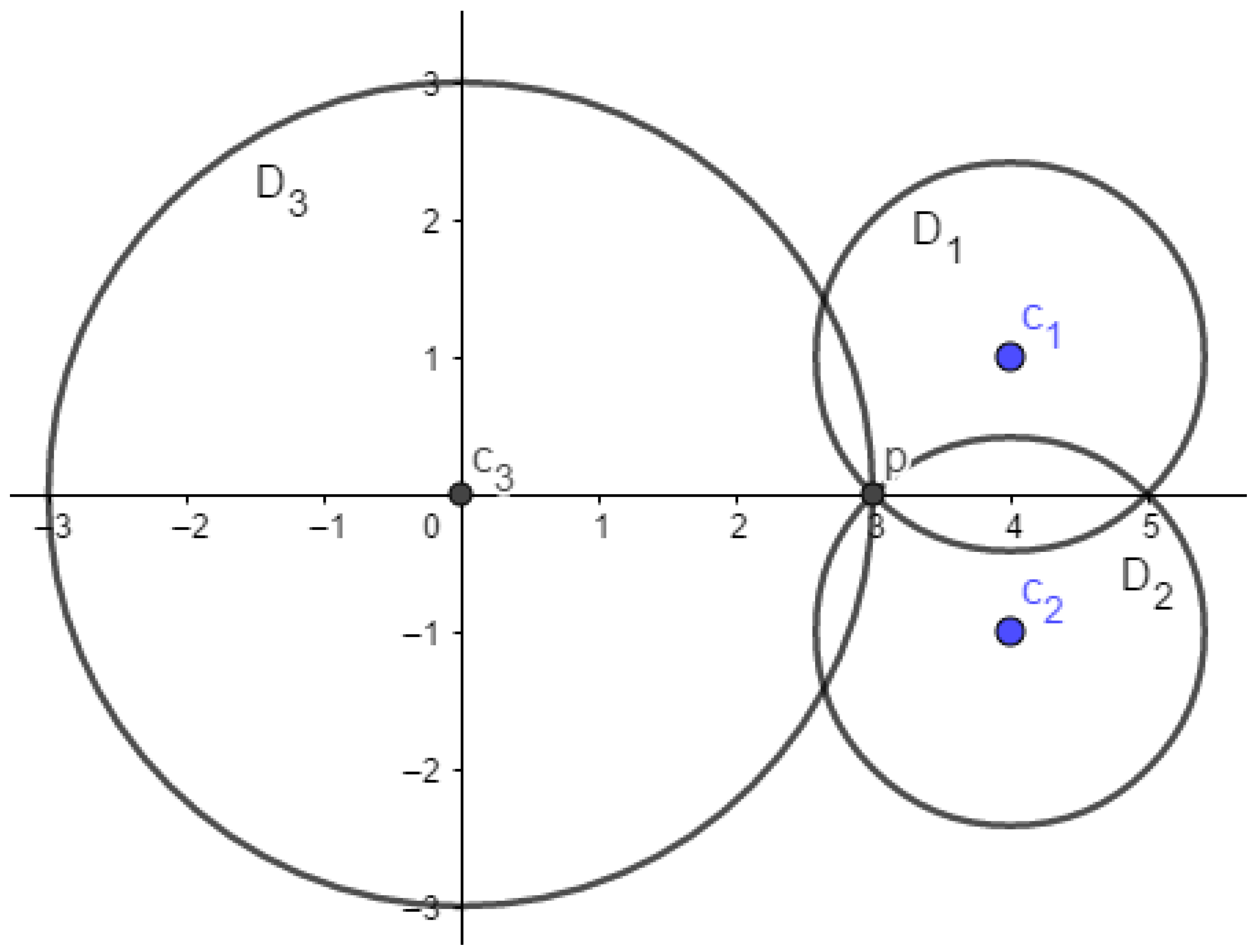
Example 1. Let

$$M=\{D_1((4,1,0);\sqrt{2}),D_2((4,-1,0);\sqrt{2}),D_3((0,0,0);3)\}\subset {\mathbb{R}}^3$$

be a Vietoris–Rips system in ${\mathbb{R}}^3$ with projection onto the $xy$-plane shown in Figure 3.

By computing the boxes $B_{i,j}$ for all $i<j$, we obtain:

$$\begin{array}{cc}\hfill B_{1,2}& =[3,5]\times [-\sqrt{2},\sqrt{2}]\times [-1,1]\hfill \\ \hfill B_{1,3}& =[4-\sqrt{2},3]\times [0,1.41]\times [-0.72,0.72]\hfill \\ \hfill B_{2,3}& =[4-\sqrt{2},3]\times [-1.4,0]\times [-0.72,0.72]\hfill \end{array}$$

Therefore, ${\cap }_{i<j}{B}_{i,j}=[3,3]\times [0,0]\times [-0.72,0.72]$. However, the disk system intersects at the point $P=(3,0,0)$, which means $AABB\left(M\right)=\left\{P\right\}$. In other words, $AABB\left(M\right)$ is not equal to ${\cap }_{i<j}{B}_{i,j}$.

We know that if $D\ne \varnothing$, then ${\cap }_{i<j}{B}_{i,j}\ne \varnothing$. However, the converse is not always true. The following example illustrates this fact.

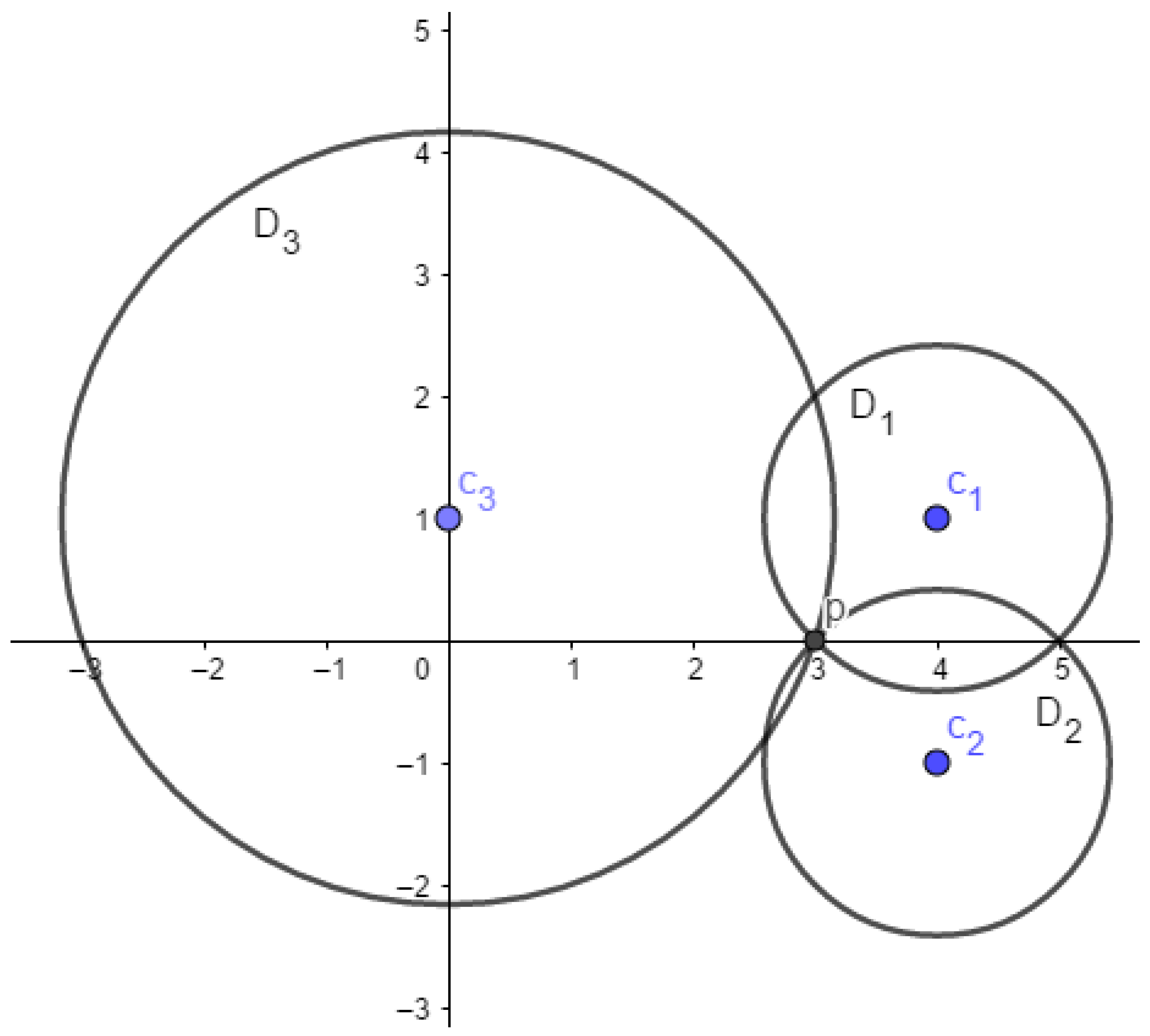
Example 2. Let $N=\{D_1,D_2,D_3((0,1,0);\sqrt{10}),D_4((3,0,1);0.9)\}\subset {\mathbb{R}}^3$ be a Vietoris–Rips system. The projection of disks $D_1,D_2,$ and $D_3$ onto the $xy$-plane is illustrated in Figure 4.

We will now compute the intersections $B_{i,j}$ for different pairs of disks:

$$\begin{array}{cc}\hfill B_{1,2}& =[3,5]\times [-\sqrt{2},\sqrt{2}]\times [-1,1]\hfill \\ \hfill B_{1,3}& =[4-\sqrt{2},\sqrt{10}]\times [0,2]\times [-1,1]\hfill \\ \hfill B_{1,4}& =[2.6,3.9]\times [-0.4,0.9]\times [0.100007,1.3]\hfill \\ \hfill B_{2,3}& =[2.6,3]\times [-0.8,0]\times [-0.44,4.47]\hfill \\ \hfill B_{2,4}& =[2.6,3.9]\times [-0.9,0.4]\times [0.100007,1.3]\hfill \\ \hfill B_{3,4}& =[2.1,3.11]\times [-0.73,0.9]\times [0.1,1.7]\hfill \end{array}$$

The intersection of all pairwise intersections, ${\cap }_{i<j}{B}_{i,j}$, is given by $[3,3]\times [0,0]\times [0.1,1.7]$. However, the intersection of disks $D_1,D_2,$ and $D_3$ is a single point P, which is not contained in $D_4$ (by construction). Therefore, D is an empty set, but ${\cap }_{i<j}{B}_{i,j}$ is not.

These examples clearly illustrate that when dealing with the AABB of three disks or more, knowing the AABB for pairs of disks is insufficient. In Example 1, we observe that the intersection of $AABB\left(\{D_i,D_j\}\right)$ is not equal to the AABB of the disk system M. Similarly, in Example 2, we find that the intersection of three disks is empty, yet the intersection of $AABB\left(\{D_i,D_j\}\right)$ contains points.

Therefore, the next crucial step is to determine how to calculate the AABB of a disk system consisting of more than two disks in ${\mathbb{R}}^d$.

4.2. Minimal Axis-Aligned Bounding Box for More Than Two Disks

Given a system M consisting of m disks in ${\mathbb{R}}^d$, we can compute the $e_q$-poles for any subcollection of disks. Using these $e_q$-poles, we can determine the Axis-Aligned Bounding Box (AABB) of M.

If $m\le d$, we calculate the $e_q$-poles of the $(d-m+1)$-sphere $\cap \partial D_i$, and with these poles, we define the AABB of M by taking $inf{\pi }_q\partial D={\pi }_q\left(p\right)$, where p is the $e_q$-south pole of the $(d-m+1)$-sphere (similarly for $sup{\pi }_q\partial D$).

In the case where $m=d+1$, we consider $AABB\left(M\right(1\left)\right),...,AABB\left(M\right(m\left)\right)$ as a collection of minimal axis-aligned boxes for the disk system $M\left(i\right)=M-\left\{D_i\right\}$ in ${\mathbb{R}}^d$. If the intersection of any $d+1$ of these sets is nonempty, then the intersection of the entire collection gives us the minimal axis-aligned box of the disk system M. This can be expressed as $AABB\left(M\right)=\cap AABB\left(M\right(i\left)\right)$. The next theorem confirms this finding.

Theorem 2 

(Helly-type theorem for minimal axis-aligned bounding boxes). Let M be a Rips system with $d+1$ disks in ${\mathbb{R}}^d$. Then, the minimal Axis-Aligned Bounding Box for the intersection set $D={\cap }_{j=1}^{d+1}{D}_j$ satisfies:

$$AABB\left(M\right)=\bigcap _{j=1}^{d+1}AABB\left(M\left(j\right)\right)$$

where $M\left(j\right)=M-\left\{D_j\right\}$.

Proof. 

We know that $AABB\left(M\right)\subseteq {\bigcap }_{j=1}^{d+1}AABB\left(M\left(j\right)\right)$. Now, our objective is to establish the reverse inclusion, i.e., ${\bigcap }_{j=1}^{d+1}AABB\left(M\left(j\right)\right)\subseteq AABB\left(M\right)$. To derive a contradiction, suppose that the reverse inclusion is not true. By definition, we have:

$$AABB\left(M\right)=\prod _{i=1}^d\left[inf{\pi }_i(\partial D),sup{\pi }_i(\partial D)\right]$$

and

$$\bigcap _{j=1}^{d+1}AABB\left(M\left(j\right)\right)=\prod _{i=1}^d\left[\underset{k}{max}\{inf{\pi }_i(\partial {\cap }_{j\ne k}{D}_j)\},\underset{k}{min}\{sup{\pi }_i(\partial {\cap }_{j\ne k}{D}_j)\}\right].$$

Without loss of generality, let us assume that:

$${\pi }_1\left(p\right)>\underset{k}{max}{\left\{inf{\pi }_1({\cap }_{j\ne k}\partial D_j)\right\}}_{k=1}^{d+1},$$

where $p\in D$ satisfies ${\pi }_1\left(p\right)=inf{\pi }_1(\partial D)$.

Let $q_j$ be the point in ${\cap }_{k\ne j}{D}_k$ such that ${\pi }_1\left(q_j\right)=inf{\pi }_1\left({\cap }_{k\ne j}{D}_k\right)$ for each $j=1,2,\cdots ,d+1$. Please note that $q_j\notin D_j$ because $q_j$ is not in D. Now, let ${\gamma }_j$ be the line segment that connects $q_j$ and p.

Choose $ϵ>0$ small enough such that the hyperplane $P:x_1={\pi }_1\left(p\right)-ϵ$ does not contain any $q_j$, and ${\pi }_1\left(q_j\right)<{\pi }_1\left(p\right)-ϵ$ for all $j=1,2,\cdots ,d+1$ (such hyperplane P exists because ${\pi }_1\left(p\right)>{\pi }_1\left(q_j\right)$ for all $j=1,\cdots ,d+1$). Since $q_j$ is in ${\cap }_{k\ne j}{D}_k$, the hyperplane P intersects every disk in $M\left(j\right)$ for each j, and ${\gamma }_j\subset {\cap }_{k\ne j}{D}_k$ intersects P at a point that is in ${\cap }_{k\ne j}{D}_k$ (see Figure 5). Furthermore, $D_k\cap P$ is a $(d-1)$-dimensional disk. Therefore, we have a collection $\mathcal{D}=\{D_j\cap P|j=1,2,\cdots ,d+1\}$ of $d+1$ disks, each of dimension $d-1$, such that every subset A of $\mathcal{D}$ consisting of d disks has the nonempty intersection property. By Helly’s Theorem, the intersection of all $(d-1)$-disks in $\mathcal{D}$ is not empty. Therefore, there exists a point $q\in D$ with ${\pi }_1\left(q\right)<{\pi }_1\left(p\right)$. However, this contradicts the fact that $p\in D$ is such that ${\pi }_1\left(p\right)=inf{\pi }_1(\partial D)$.

Therefore, we conclude that ${\bigcap }_{j=1}^{d+1}AABB\left(M\left(j\right)\right)=AABB\left(M\right)$.    □

Lemma 6. 

Let M be a Vietoris–Rips system of $d+1$ disks in ${\mathbb{R}}^d$. If $D={\cap }_{i=1}^{d+1}{D}_i=\varnothing$ and $AABB\left(M\right(j\left)\right)\ne \varnothing$ for each $j=1,\cdots ,d+1$, then ${\cap }_{i=1}^{d+1}AABB\left(M\left(i\right)\right)$ consists only of intervals of the form $[a,b]$ with $a>b$ (inverted intervals).

Proof. 

Suppose that ${\cap }_{i=1}^{d+1}AABB\left(M\left(i\right)\right)$ contains an interval. Without loss of generality, let us assume it is the interval

$$[inf{\pi }_1(\partial D\left(k\right)),sup{\pi }_1(\partial D\left(l\right))],$$

for some $k,l\in \{1,2,\cdots ,d+1\}$, where $D\left(k\right)={\cap }_{i\ne k}{D}_i$. By definition of ${\cap }_{i=1}^{d+1}AABB\left(M\left(i\right)\right)$, we have $inf{\pi }_1(\partial D\left(k\right))\ge inf{\pi }_1(\partial D\left(i\right))$ for all $i\ne k$ and $sup{\pi }_1(\partial D\left(l\right))\le sup{\pi }_1(\partial D\left(j\right))$ for all $j\ne l$. Now, consider a hyperplane $P:x_1=p$ with $inf{\pi }_1(\partial D\left(k\right))\le p\le sup{\pi }_1(\partial D\left(k\right))$. The hyperplane P intersects $D\left(j\right)$ for every $j=1,\cdots ,d+1$ (since P cuts through all the boxes $AABB\left(M\right(j\left)\right)$). We also know that $P\cap D_i$ is a $d-1$-dimensional disk for each i.

Therefore, we have a collection of d disks in a $d-1$-dimensional space, and by Helly’s Theorem, this collection must have a nonempty intersection. This implies that $D\ne \varnothing$, which contradicts our assumption that D is empty. Hence, all intervals in ${\cap }_{i=1}^{d+1}AABB\left(M\left(i\right)\right)$ must be inverted intervals of the form $[a,b]$ with $a>b$.    □

As an example, we provide the lower bounds of the AABB for a system of three disks in ${\mathbb{R}}^d$, i.e., we compute $inf{\pi }_i(\partial D)$ for each $i=1,\cdots ,d$ (analogous $sup{\pi }_i\partial D$) with $D={\cap }_{j=1}^3{D}_j$. Let $M=\{D_1,D_2,D_3\}$ be a Rips system in ${\mathbb{R}}^d$, then, for each $i=1,\cdots ,d$, the computation of the AABB for the disk system M is given by:

$$\begin{array}{c}\hfill inf{\pi }_i(\partial D)=\left\{\begin{array}{cc}{\pi }_i(c_k-r_k{e}_i)\hfill & \mathrm{if}{c}_k-r_k{e}_i\in D\hfill \\ \underset{j<k}{max}\{inf{\pi }_i(\partial D_j\cap \partial D_k)\}\hfill & \mathrm{if}(*)\hfill \\ inf{\pi }_i({\cap }_{j=1}^3\partial D_j)\hfill & \mathrm{otherwise}\hfill \end{array}\right.\end{array}$$

where (*) denotes the case where $q\in D$ with $q\in \partial D_j\cap \partial D_k$ such that

$${\pi }_i\left(q\right)=\underset{j<k}{max}\{inf{\pi }_i(\partial D_j\cap \partial D_k)\}.$$

The preceding calculations are a result of Lemma 2. It is known that the extremes of the AABB lie in the projections of specific poles, either from a d-sphere, $(d-1)$-sphere, or the $(d-2)$-sphere.

Given a disk system M in ${\mathbb{R}}^d$, we can compute the minimal Axis-Aligned Bounding Box (AABB) for the intersection of all disks in M. If the AABB is a point, then it represents the intersection of the disks. This property allows us to identify when the AABB is a point. If the AABB of M is not a point, we can rescale M by a scale factor $\lambda$ such that the AABB of $M_{\lambda }$ becomes a point. The value of $\lambda$ is referred to as the Čech scale of the system M.

4.3. Minimal Axis-Aligned Bounding Box Algorithm

Now, we present an algorithm (Algorithm 3: AABB.minimal) to calculate the minimal Axis-Aligned Bounding Box (AABB) of a system of m disks in ${\mathbb{R}}^d$. As previously explained, the AABB’s extremes are defined by projecting the poles of specific i-spheres. Thus, in computing the AABB, we will determine the poles for each i-sphere within the disk system.

The Algorithm 3 starts by initializing the set of poles, P, as an empty set. In each iteration of the first loop, we determine the spheres formed by the intersection of the boundaries of the disk subcollections in the system M (for this, we require the center and radius, which are computed in Section 2.2). Next, we identify the poles of each sphere, and if any of them are present in all the disks of M, we add them to the set P. If P is not empty, we proceed to calculate the extremes for each dimension of the AABB using the set of north poles for the upper bounds and the set of south poles for the lower bounds. In this case, the output is the product of the intervals defined by the computed extremes. If P is empty, it indicates that there is no intersection in the disk system.

Algorithm 3:AABB.minimal

5. Conclusions

Addressing the problem of computing the Čech filtration for a finite disk system, as well as the computation of the minimal Axis-Aligned Bounding Box (AABB) for the intersection of such a disk system, in this paper, we have designed three algorithms: Cech.system (a TRUE/FALSE test to indicate whether a disk system has a nonempty intersection), Cech.scale (a numerical method approach to approximate the Čech scale of a disk system with any given precision), and AABB.minimal (an exhaustive search algorithm for $e_q$-poles whose output is the minimal AABB for the intersection of the disks in any disk system). The algorithms we have described are fundamentally based on Lemmas 1 and 2 in Section 2. The latter is a key result for this work, as it directs our attention to a finite collection of points: the north/south poles of spheres of different dimensions, which are determined by the intersection of other spheres. These points allow us to sufficiently characterize the intersection of a finite collection of disks so that it can be bounded by axis-aligned boxes and to determine if such an intersection is nonempty. Furthermore, to make this result computable (as required in applications, such as topological data analysis), we have developed explicit formulae for computing such poles in Section 2.1 and Section 2.2.