


Investigating Behavior of Slider–Crank Mechanisms with Bearing Failures Using Vibration Analysis Techniques
Abstract
1. Introduction
2. Mathematical Model
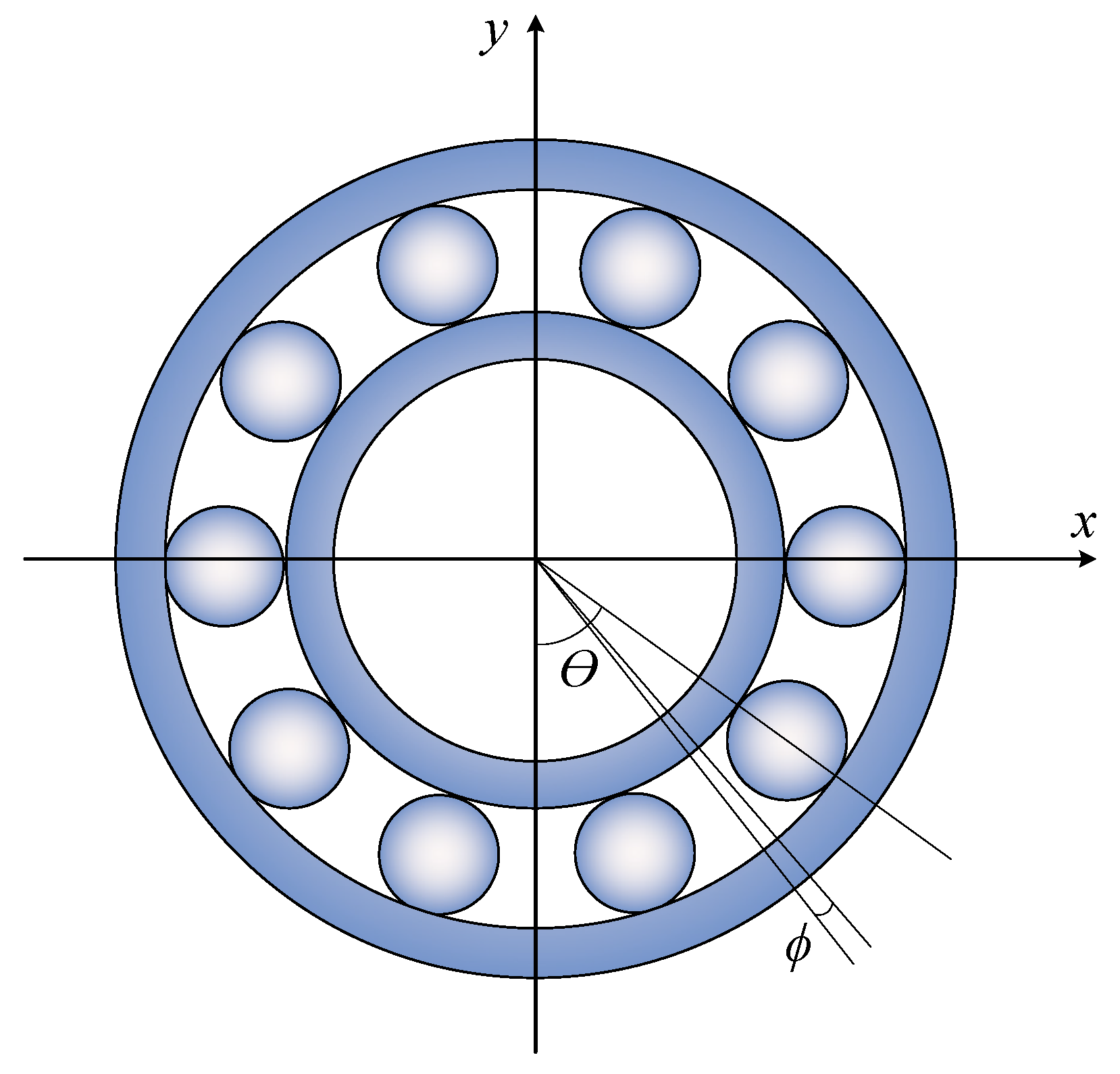
2.1. System Modeling for the Ball Bearings
2.2. Calculating the Forces
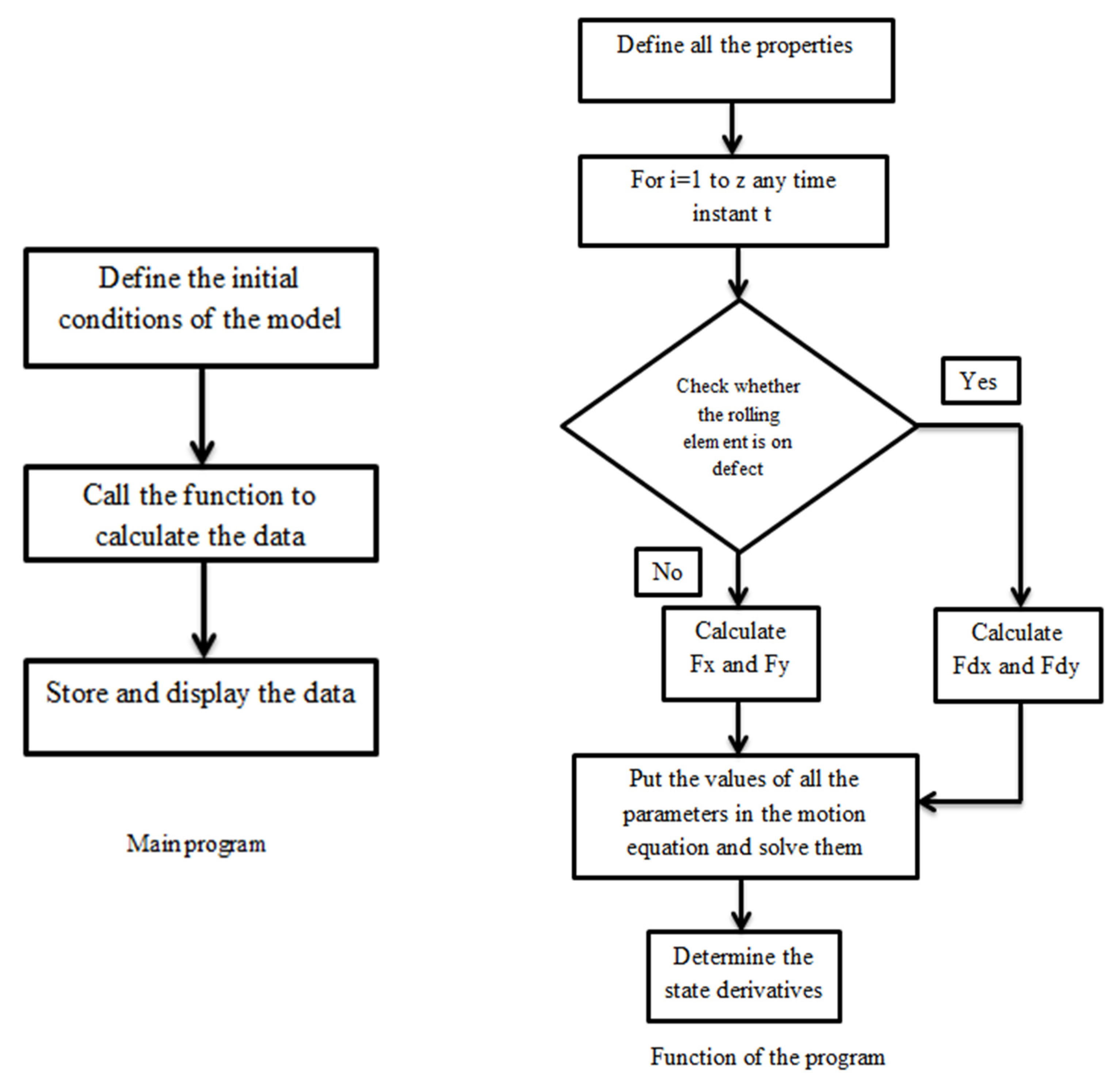
2.3. MATLAB Program to Determine the State Variables for Roller Bearings
2.4. System Modeling for the Roller Bearings
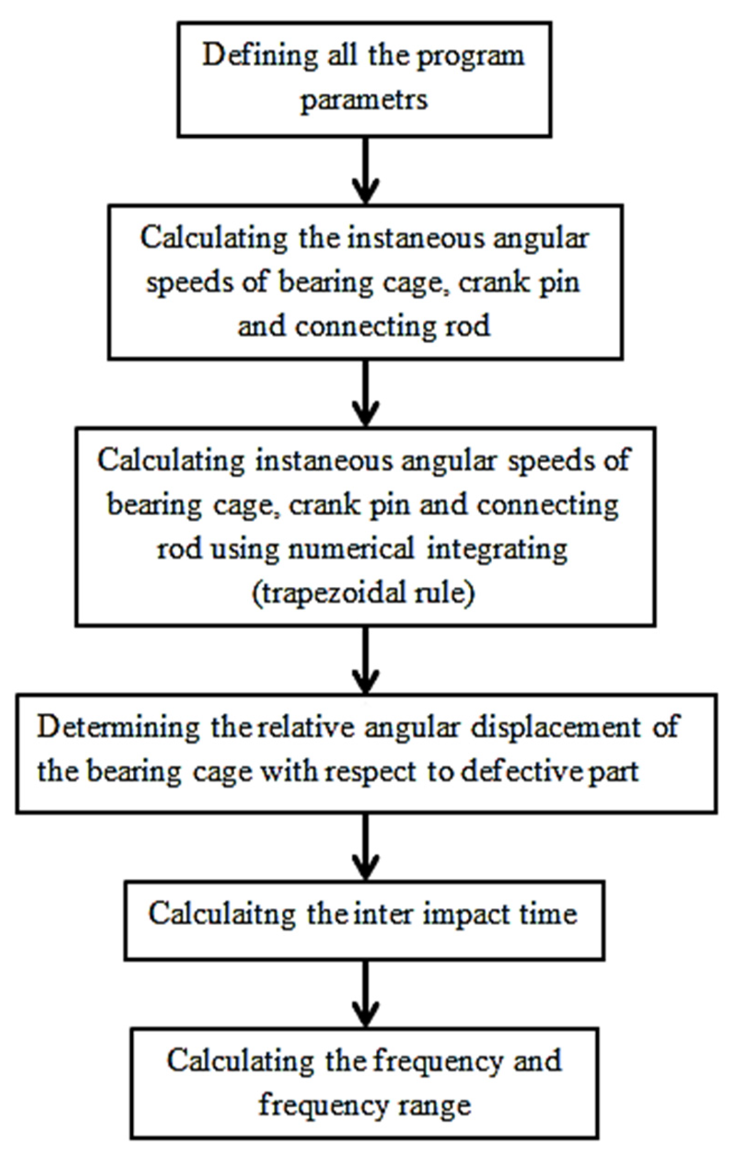
2.5. The MATLAB Program to Determine the Frequency Range
3. Experimental Setup
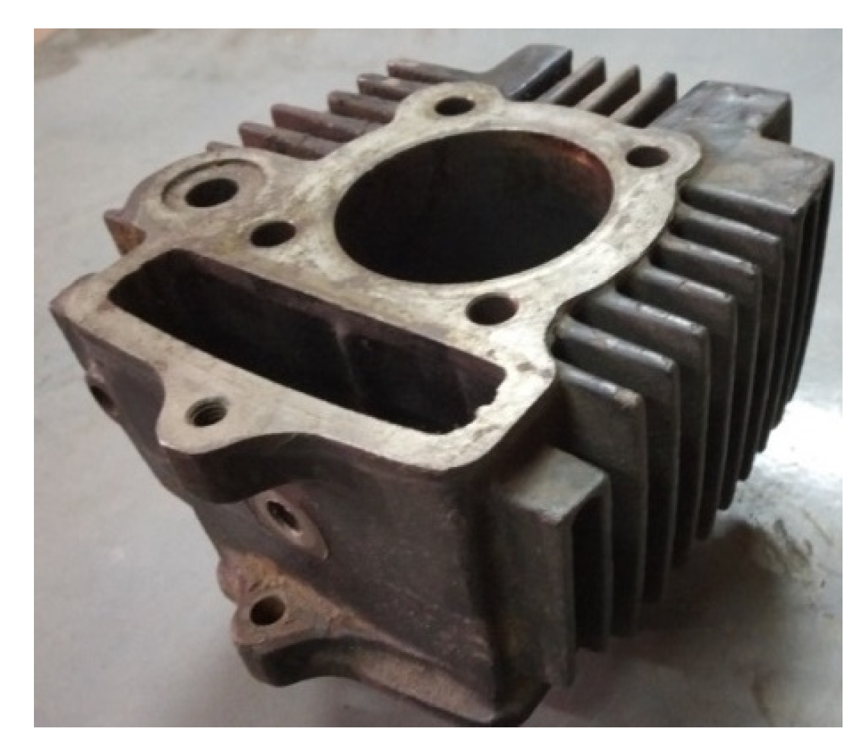
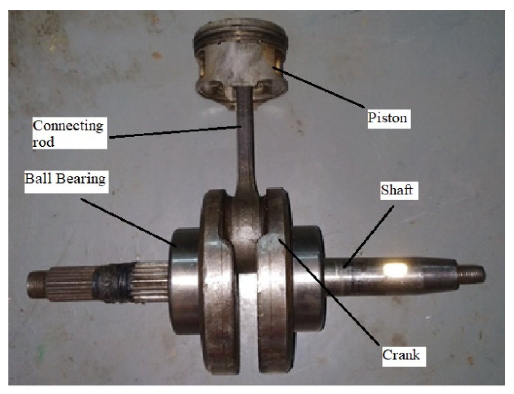
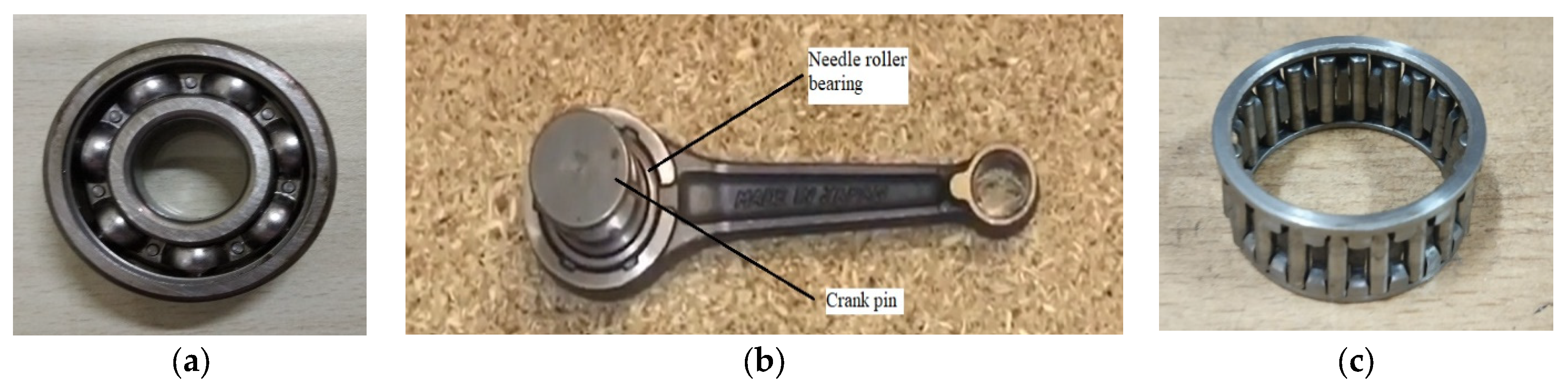
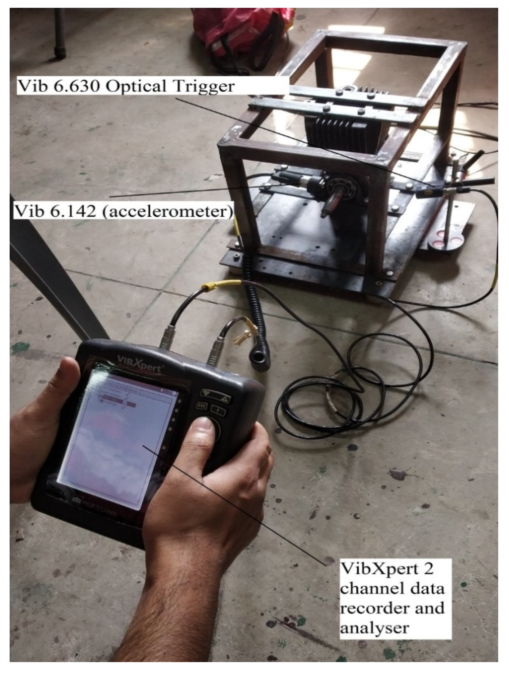
3.1. Experiment Equipment
3.2. Experimental Procedure
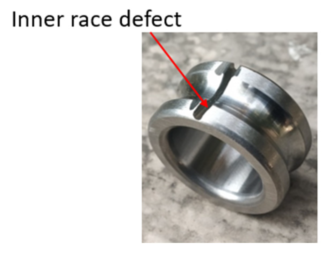
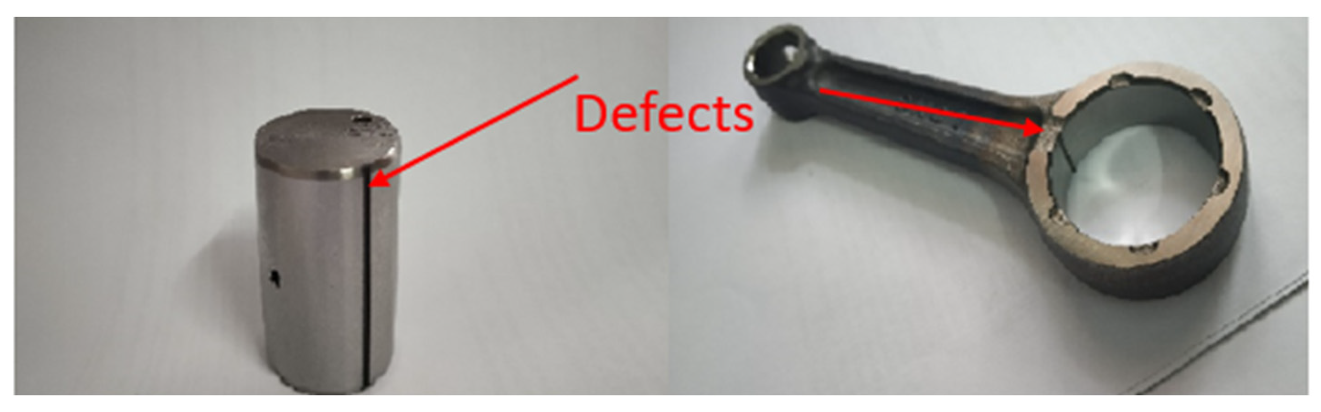
3.3. Inducing Damage
3.4. Data Acquisition and Accelerometer
4. Results and Discussions
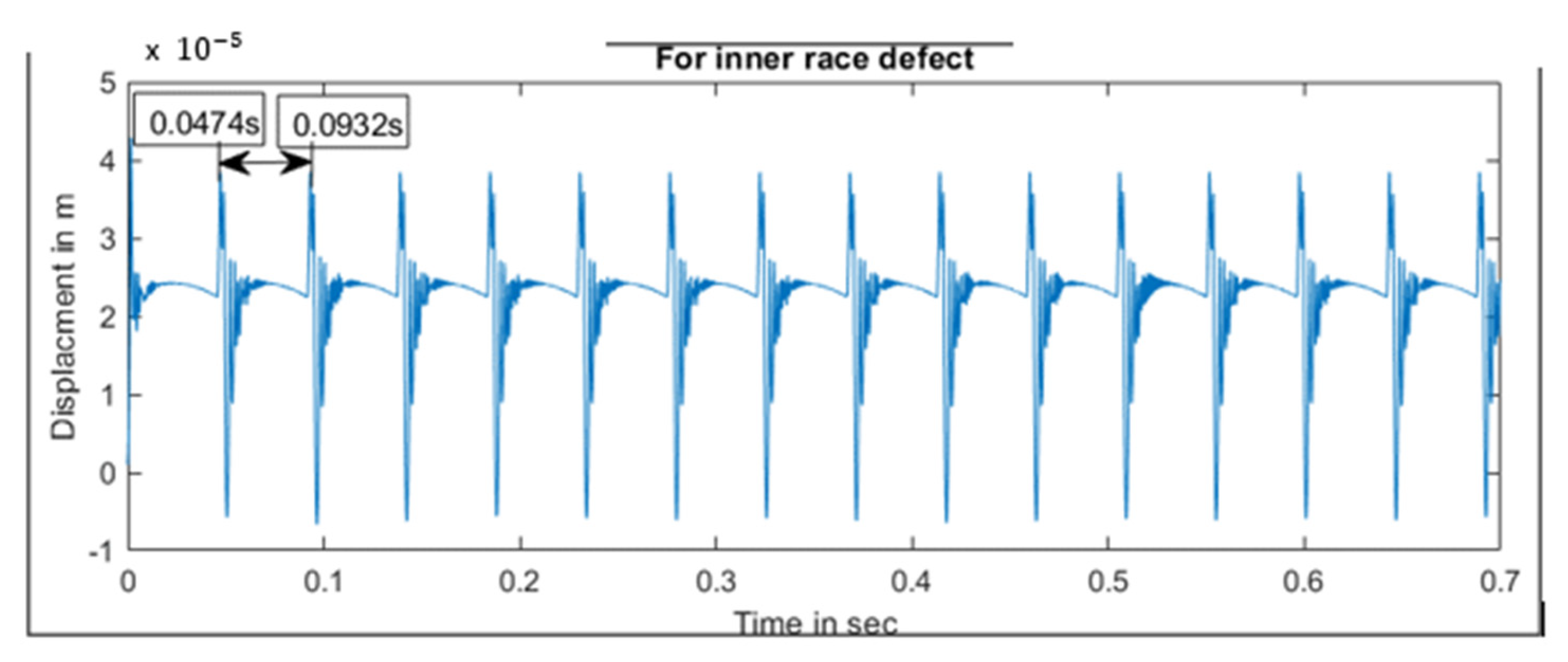
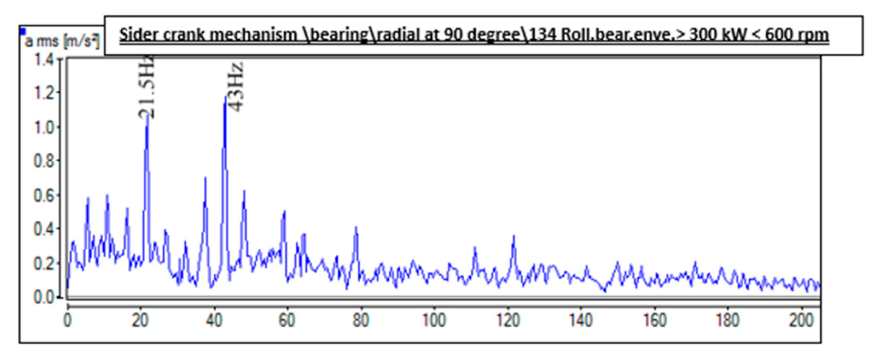
4.1. Results for the Analysis of Defect in Ball Bearing
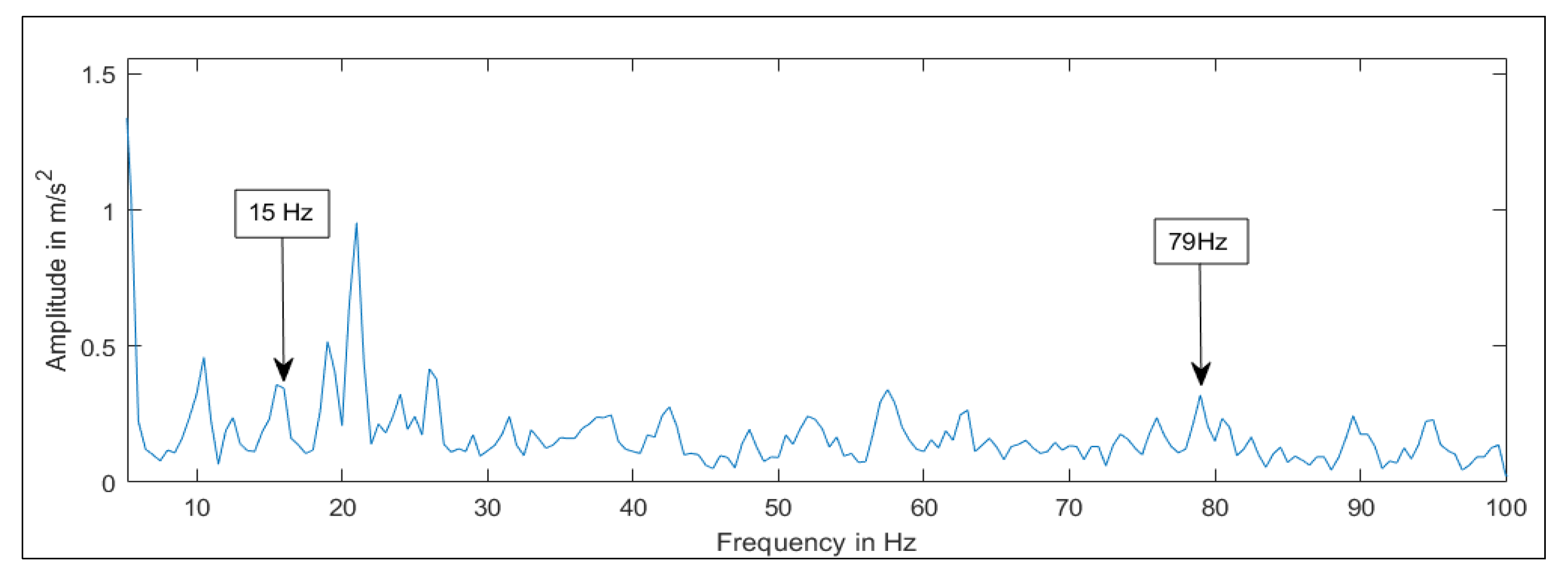
4.2. Results for the Analysis of Defects of Needle Roller Bearing
5. Conclusions
Author Contributions
Funding
Data Availability Statement
Acknowledgments
Conflicts of Interest
References
- Butler, D.E. The Shock-pulse method for the detection of damaged rolling bearings. Non-Destr. Test. 1973, 6, 92–95. [Google Scholar] [CrossRef]
- Gupta, P.K. Dynamics of rolling-element bearings part I: Cylindrical roller bearing analysis discussion. J. Tribol. 1979, 101, 293–302. [Google Scholar] [CrossRef]
- Gupta, P.K. Dynamics of Rolling Element Bearings—2. Cylindrical Roller Bearing Results. Am. Soc. Mech. Eng. 1978, 101, 305–311. [Google Scholar] [CrossRef]
- Toersen, H. Application of an envelope technique in the detection of ball bearing defects in a laboratory experiment. TriboTest 1998, 4, 297–308. [Google Scholar] [CrossRef]
- McFadden, P.D.; Smith, J.D. Model for the vibration produced by a single point defect in a rolling element bearing. J. Sound Vib. 1984, 96, 69–82. [Google Scholar] [CrossRef]
- Patil, M.S.; Mathew, J.; Rajendrakumar, P.K.; Desai, S. A theoretical model to predict the effect of localized defect on vibrations associated with ball bearing. Int. J. Mech. Sci. 2010, 52, 1193–1201. [Google Scholar] [CrossRef]
- Tandon, N.; Choudhury, A. An analytical model for the prediction of the vibration response of rolling element bearings due to a localized defect. J. Sound Vib. 1997, 205, 275–292. [Google Scholar] [CrossRef]
- Liu, J.; Shao, Y.; Lim, T.C. Vibration analysis of ball bearings with a localized defect applying piecewise response function. Mech. Mach. Theory 2012, 56, 156–169. [Google Scholar] [CrossRef]
- Choudhury, A.; Tandon, N. Application of acoustic emission technique for the detection of defects in rolling element bearings. Tribol. Int. 2000, 33, 39–45. [Google Scholar] [CrossRef]
- Rubini, R.; Meneghetti, U. Application of the envelope and wavelet transform analyses for the diagnosis of incipient faults in ball bearings. Mech. Syst. Signal Process. 2001, 15, 287–302. [Google Scholar] [CrossRef]
- Kiral, Z.; Karagülle, H. Simulation and analysis of vibration signals generated by rolling element bearing with defects. Tribol. Int. 2003, 36, 667–678. [Google Scholar] [CrossRef]
- Rai, V.K.; Mohanty, A.R. Bearing fault diagnosis using FFT of intrinsic mode functions in Hilbert-Huang transform. Mech. Syst. Signal Process. 2007, 21, 2607–2615. [Google Scholar] [CrossRef]
- Lu, S.; Wang, X.; He, Q.; Liu, F.; Liu, Y. Fault diagnosis of motor bearing with speed fluctuation via angular resampling of transient sound signals. J. Sound Vib. 2016, 385, 16–32. [Google Scholar] [CrossRef]
- Cui, L.; Zhang, Y.; Zhang, F.; Zhang, J.; Lee, S. Vibration response mechanism of faulty outer race rolling element bearings for quantitative analysis. J. Sound Vib. 2016, 364, 67–76. [Google Scholar] [CrossRef]
- Patel, V.N.; Tandon, N.; Pandey, R.K. Dynamic model for vibration studies of deep groove ball bearings considering single and multiple defects in races. J. Tribol. 2010, 132, 041101. [Google Scholar] [CrossRef]
- Salunkhe, V.G.; Desavale, R.G.; Kumbhar, S.G. Vibration Analysis of Deep Groove Ball Bearing Using Finite Element Analysis and Dimension Analysis. J. Tribol. 2022, 144, 081202. [Google Scholar] [CrossRef]
- Nan, G.; Jiang, S.; Yu, D. Dynamic analysis of rolling ball bearing-rotor based on a new improved model. SN Appl. Sci. 2022, 4, 173. [Google Scholar] [CrossRef]
- Hou, D.; Qi, H.; Luo, H.; Wang, C.; Yang, J. Comparative study on the use of acoustic emission and vibration analyses for the bearing fault diagnosis of high-speed trains. Struct. Health Monit. 2022, 21, 1518–1540. [Google Scholar] [CrossRef]
- AbdulBary, M.; Embaby, A.; Gomaa, F. Fault Diagnosis in Rotating System Based on Vibration Analysis. ERJ. Eng. Res. J. 2021, 44, 285–294. [Google Scholar] [CrossRef]
- Xiao, S.; Xiao, Q.; Song, M.; Zhang, Z. Dynamic analysis for a reciprocating compressor system with clearance fault. Appl. Sci. 2021, 11, 1295. [Google Scholar] [CrossRef]
- Jangra, D. A Review on Different Faults in Gearbox and Vibration Based Diagnosis. Int. J. Curr. Eng. Technol. 2022, 12, 315–325. [Google Scholar] [CrossRef]


| Quantities | Values |
|---|---|
| Hertzian contact load | |
| Radial clearance | |
| Radial load | |
| Damping coefficient | |
| Mass of outer race | |
| For inner race | |
| Shaft speed | |
| Relative cage speed | |
| Length of defect | |
| Angular length of defect | |
| Height of defect | |
| For outer race | |
| Shaft speed | |
| Cage speed | |
| Length of defect | |
| Angular length of defect | |
| Height of defect | |
| For rolling element | |
| Shaft speed | |
| Cage speed | |
| Length of defect | |
| Average angular length of defect | |
| Height of defect | |
| Initial displacement in | |
| Initial velocity in | |
| Initial displacement in | |
| Initial velocity in | |
| Time for simulation | |
| Time step |
| Quantity | Values |
|---|---|
| Crank radius | 24.5 mm |
| Connection rod length | 94 m |
| Rolling element diameter | 2.5 mm |
| Pitch diameter | 27.5 m |
| Number of rolling element | 20 |
| Inter-impact angular distance | 0.314159265 |
| Shaft speed for crack pin defect | 314 rpm |
| Shaft speed for connecting rod defect | 313 rpm |
| Setup Class | Bearing Spectrum |
|---|---|
| Quantity | Acceleration |
| HP/LP Filter | 1000/40,000 |
| Frequency | 400 Hz |
| Line No. | 800 |
| Window | Hanning |
| Envelope | On |
| Averages | 3 (Linear) |
| Defect Types | Calculated Defective Operating Frequency | Experimental Frequency |
|---|---|---|
| Inner race defect | 21.83 Hz | 21.5 Hz |
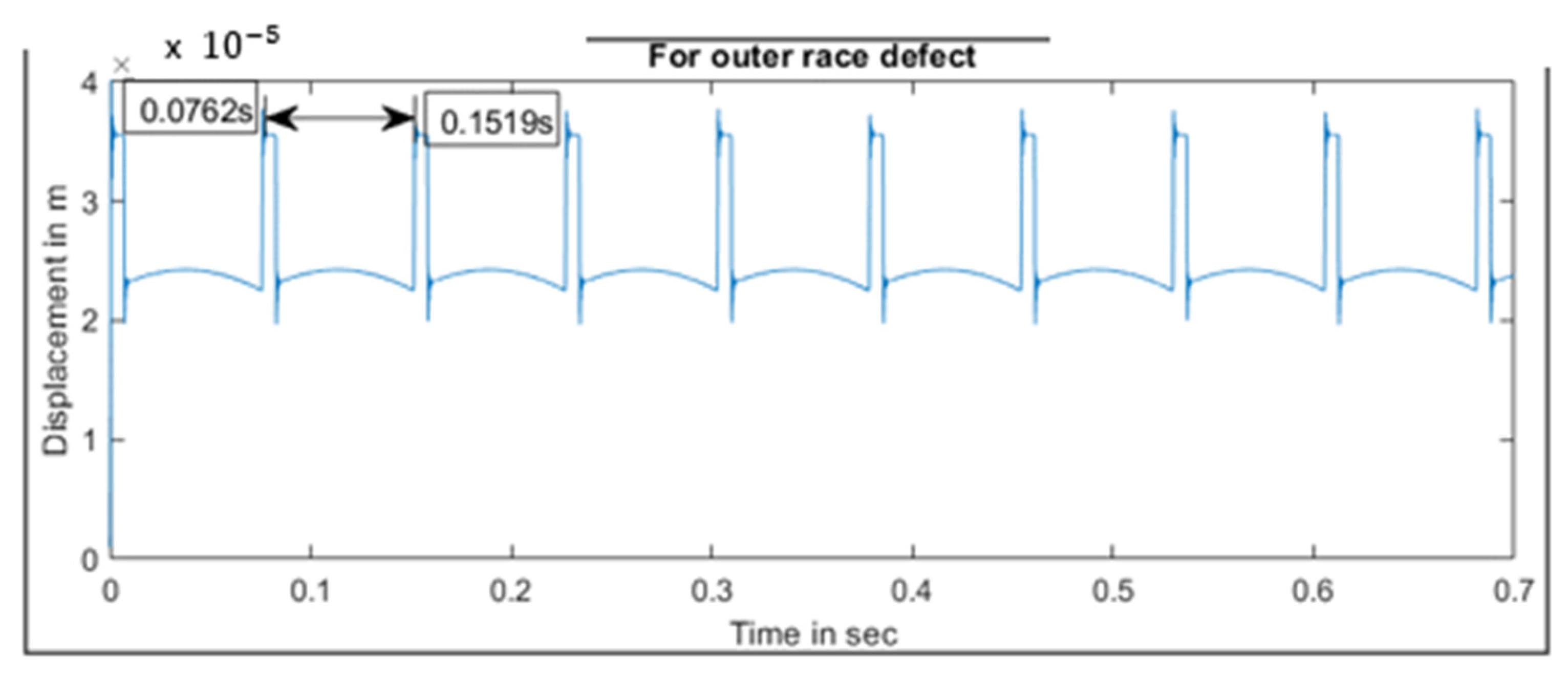
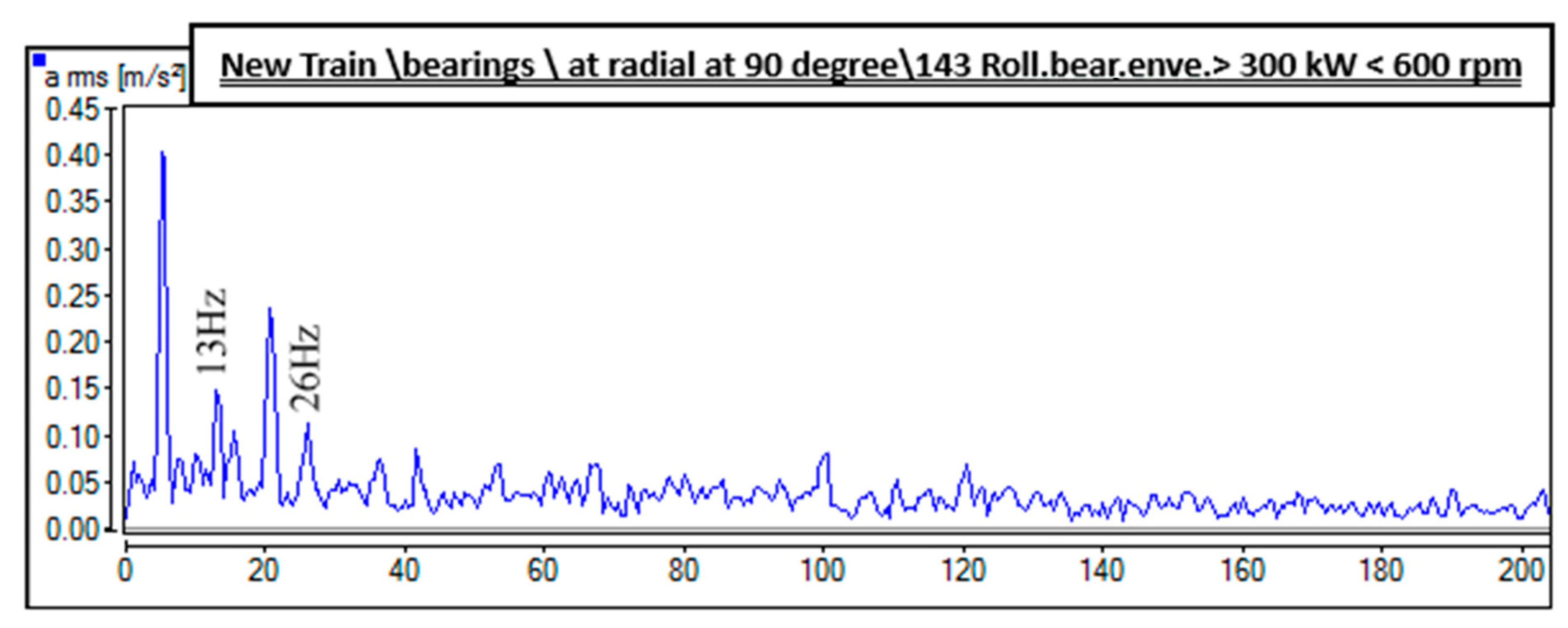
| Outer race defect | 13.21 Hz | 13 Hz |
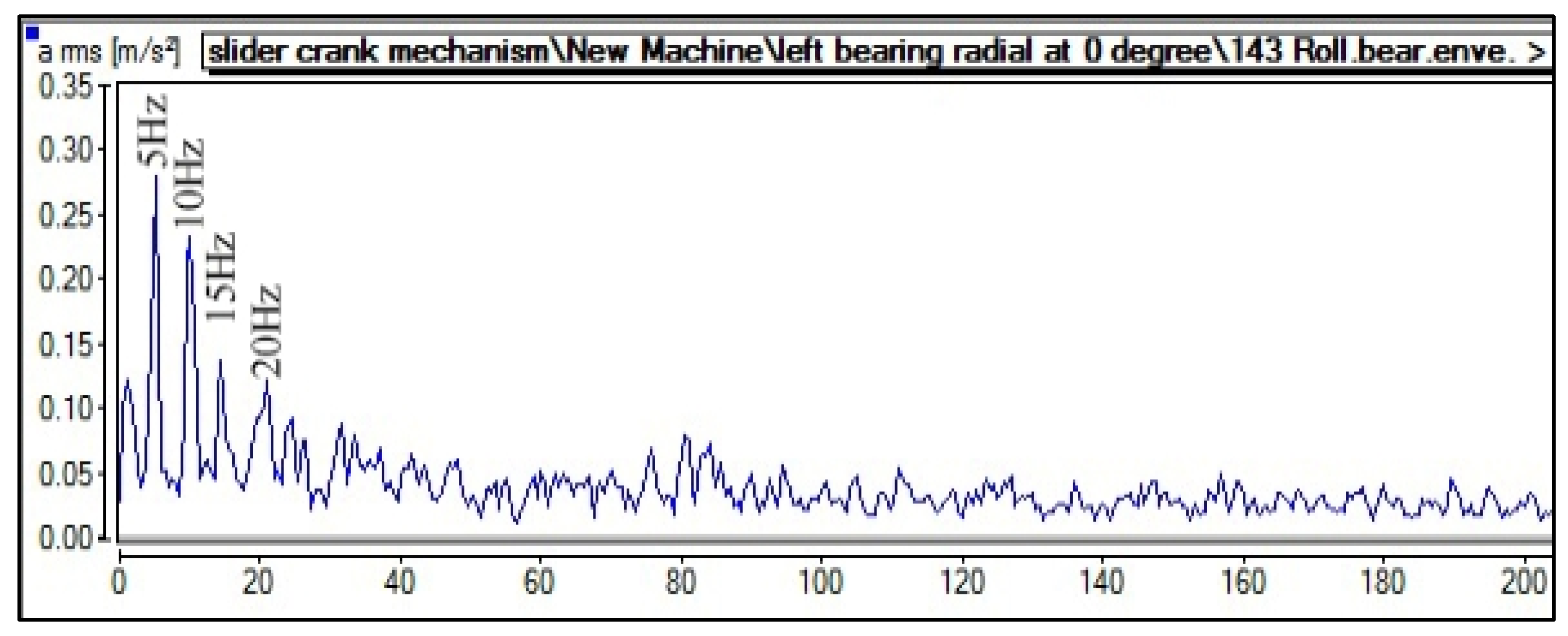
| Ball defect | 9.18 Hz | 9.5 Hz |
| Defect Types | Calculated Defective Frequency Range | Experimental Defective Frequency Range |
|---|---|---|
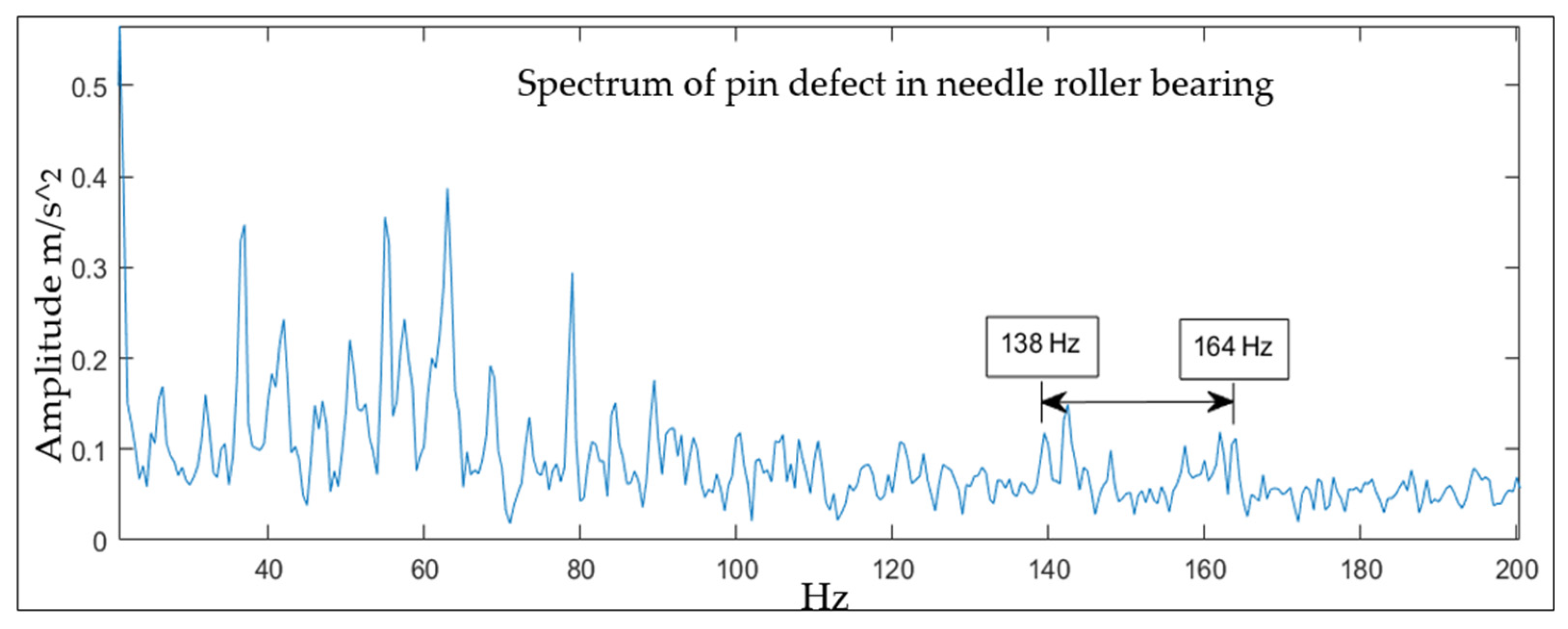
| Pin defect | 137–167 Hz | 138–164 Hz |
| Connecting rod defect | 14–82 Hz | 15–79 Hz |
Disclaimer/Publisher’s Note: The statements, opinions and data contained in all publications are solely those of the individual author(s) and contributor(s) and not of MDPI and/or the editor(s). MDPI and/or the editor(s) disclaim responsibility for any injury to people or property resulting from any ideas, methods, instructions or products referred to in the content. |
© 2024 by the authors. Licensee MDPI, Basel, Switzerland. This article is an open access article distributed under the terms and conditions of the Creative Commons Attribution (CC BY) license (https://creativecommons.org/licenses/by/4.0/).
Share and Cite
Ghazwani, M.H.; Pham, V.V. Investigating Behavior of Slider–Crank Mechanisms with Bearing Failures Using Vibration Analysis Techniques. Mathematics 2024, 12, 544. https://doi.org/10.3390/math12040544
Ghazwani MH, Pham VV. Investigating Behavior of Slider–Crank Mechanisms with Bearing Failures Using Vibration Analysis Techniques. Mathematics. 2024; 12(4):544. https://doi.org/10.3390/math12040544
Chicago/Turabian StyleGhazwani, Mofareh Hassan, and Van Vinh Pham. 2024. "Investigating Behavior of Slider–Crank Mechanisms with Bearing Failures Using Vibration Analysis Techniques" Mathematics 12, no. 4: 544. https://doi.org/10.3390/math12040544
APA StyleGhazwani, M. H., & Pham, V. V. (2024). Investigating Behavior of Slider–Crank Mechanisms with Bearing Failures Using Vibration Analysis Techniques. Mathematics, 12(4), 544. https://doi.org/10.3390/math12040544