Article

A Comprehensive Multi-Strategy Enhanced Biogeography-Based Optimization Algorithm for High-Dimensional Optimization and Engineering Design Problems

1
School of Computer Science and Engineering, Xidian University, Xi’an 710071, China
2
Ningxia Province Key Laboratory of Intelligent Information and Data Processing, North Minzu University, Yinchuan 750021, China
*
Author to whom correspondence should be addressed.
Mathematics 2024, 12(3), 435; https://doi.org/10.3390/math12030435
Submission received: 15 December 2023 / Revised: 19 January 2024 / Accepted: 23 January 2024 / Published: 29 January 2024
(This article belongs to the Special Issue Smart Computing, Optimization and Operations Research)

Abstract

:
The biogeography-based optimization (BBO) algorithm is known for its simplicity and low computational overhead, but it often struggles with falling into local optima and slow convergence speed. Against this background, this work presents a multi-strategy enhanced BBO variant, named MSBBO. Firstly, the example chasing strategy is proposed to eliminate the destruction of the inferior solutions to superior solutions. Secondly, the heuristic crossover strategy is designed to enhance the search ability of the population. Finally, the prey search–attack strategy is used to balance the exploration and exploitation. To verify the performance of MSBBO, we compare it with standard BBO, seven BBO variants (PRBBO, BBOSB, HGBBO, FABBO, BLEHO, MPBBO and BBOIMAM) and seven meta-heuristic algorithms (GWO, WOA, SSA, ChOA, MPA, GJO and BWO) on multiple dimensions of 24 benchmark functions. It concludes that MSBBO significantly outperforms all competitors both on convergence accuracy, speed and stability, and MSBBO basically converges to the same results on 10,000 dimensions as on 1000 dimensions. Further, MSBBO is applied to six real-world engineering design problems. The experimental results show that our work is still more competitive than other latest optimization techniques (COA, EDO, OMA, SHO and SCSO) on constrained optimization problems.

1. Introduction

With the development of engineering technology and science, the optimization problem has been widely existent in all aspects of social production. In order to solve different optimization problems, various optimization techniques have been designed. They are all involved in problems where there are optimal solutions, such as robot path planning [1], vehicle routing [2], portfolio optimization [3], job-shop scheduling [4], array antenna optimization [5], etc. The purpose of optimization is to reduce cost consumption, improve economic returns, enhance system efficiency, save time, etc. At present, a relatively complete optimization system has been formed, which mainly uses mathematical methods to provide solutions to various problems. These methods are mainly divided into two categories: traditional optimization technology and meta-heuristic algorithm. Traditional optimization methods rely more on the known information of the problem to solve the deterministic problem effectively, such as the branch and bound algorithm [6], conjugate gradient method [7], steepest descent method [8], etc. Unlike these techniques, meta-heuristic algorithms obtain new optimization models by simulating certain natural phenomena or animal behaviors. Meta-heuristic algorithms can not only solve NP-hard problems but also find the optimal solution in finite time, and do not need the gradient information of the problem, so they are more suitable for nonlinear and complex optimization problems. They meet the requirements of current optimization problems and become mainstream optimization methods.
As shown in Figure 1, meta-heuristic algorithms can be roughly divided into five categories according to different classification standards: evolution-based optimization algorithms, such as the genetic algorithm (GA) [9], differential evolution (DE) [10] and immune algorithm (IA) [11]; population-based optimization algorithms, such as particle swarm optimization (PSO) [12], whale optimization algorithm (WOA) [13] and sparrow search algorithm (SSA) [14]; nature-based optimization algorithms, such as biogeography-based optimization (BBO) [15], invasive weed optimization (IWO) [16] and tree seed algorithm (TSA) [17]; physics-based optimization algorithms, such as the Archimedes optimization algorithm (AOA) [18], Kepler optimization algorithm (KOA) [19] and Young’s double-slit experiment optimizer (YDSE) [20]; and human-based optimization algorithms, such as student psychology-based optimization (SPBO) [21], teaching and learning optimization (TLO) [22] and human behavior-based optimization (HBBO) [23]. Different meta-heuristic algorithms have different performance in solving different types of optimization problems. These existing meta-heuristic algorithms have been widely used in various fields of manufacturing. However, with the rapid development of the information age, the complexity of the problems faced by human beings is different from the past, and gradually tends to be high dimensional and large scale. According to the investigation, problems with more than 100 dimensions are considered high-dimensional optimization problems [24,25,26]. But the vast majority of meta-heuristic algorithms have not been used to solve optimization problems with more than 100 dimensions. Therefore, in this context, it is still necessary to improve the existing meta-heuristic algorithm to solve the optimization problem of higher dimensions.
The BBO algorithm is a novel meta-heuristic algorithm proposed by Simon in “IEEE TEVC” in 2008 [15]. The BBO algorithm simulates the movement of species between different habitats in nature. Due to its simple principle and few parameters, BBO attracted many scholars once it was proposed and has been widely used in various fields [27,28,29,30]. Compared with other meta-heuristic algorithms, BBO has the following advantages: (1) BBO uses the migration operator to complete the variable exchange between candidate solutions, which is more ergodic than the crossover operator. When the dimension of the optimization problem is high, it can still search for the optimal direction in each dimension. (2) BBO does not need to adjust parameters, as the only two parameters are fixed. In other words, when solving high-dimensional optimization problems, the parameters will not affect the algorithm performance of BBO. This is more convenient than PSO, DE and other algorithms. (3) BBO can take advantage of the useful information carried by the current population. Unlike other meta-heuristic algorithms, the BBO candidate solution variables come from all population individuals. This enables the BBO to search adequately, even in high-dimensional environments. Based on the above discussion, we can find that BBO has more obvious advantages than other meta-heuristic algorithms in solving high-dimensional optimization problems. Therefore, based on the unique advantages of BBO, we choose to use BBO to challenge the efficient solution of high-dimensional optimization problems. This is also the motivation of choosing BBO in this paper.
However, according to the “no free lunch” principle, the BBO algorithm is not perfect. Similar to many meta-heuristic algorithms, BBO has some shortcomings, such as slow convergence speed, premature convergence, and falling into local optima. In recent years, researchers have proposed various BBO variants to improve its performance and prevent premature convergence [31]. For example, Ergezer [32] designed the OBBO algorithm based on the opposition-based learning (OBL) strategy for the first time. Experimental results show that the probability of obtaining the optimal solution of the problem is much better than that of the standard BBO algorithm. Wang et al. [33] designed a biogeography-based krill herd (BBKH) algorithm to solve complex optimization problems. The main improvement is to introduce a new krill migration operator to deal with nonlinear problems more efficiently. Lohokare et al. [34] adopted an improved mutation function to embed the neighborhood mutation of DE into BBO, thus accelerating the convergence of BBO. In their study, when the authors evaluated the performance of their proposed approach on benchmark test suite and economical load scheduling problems, their improved BBO outperformed the standard BBO. In order to reduce the dependence of BBO on the coordinate system of the optimization problem, Chen et al. [35] developed a variant of BBO based on covariance matrix migration. Experiments show that this method is superior to previous BBO variants. Then, Sang et al. [36] proposed DCGBBO by a hierarchical tissue-like P system with triggering ablation rules, making use of the evolution rule and communication rule to achieve migration and mutation, which reduces the computational complexity. Recently, to enhance the overall performance of BBO algorithm, [37] designed a novel BBO variant with hybrid migration operator and feedback differential evolution mechanism, referred to as HFBBO. It is a “living algorithm” that can self-regulate the mutation mode. The HFBBO feedback differential evolution mechanism is designed to replace the random mutation operator, so the population can select the mutation mode intelligently to avoid falling into the local optima.
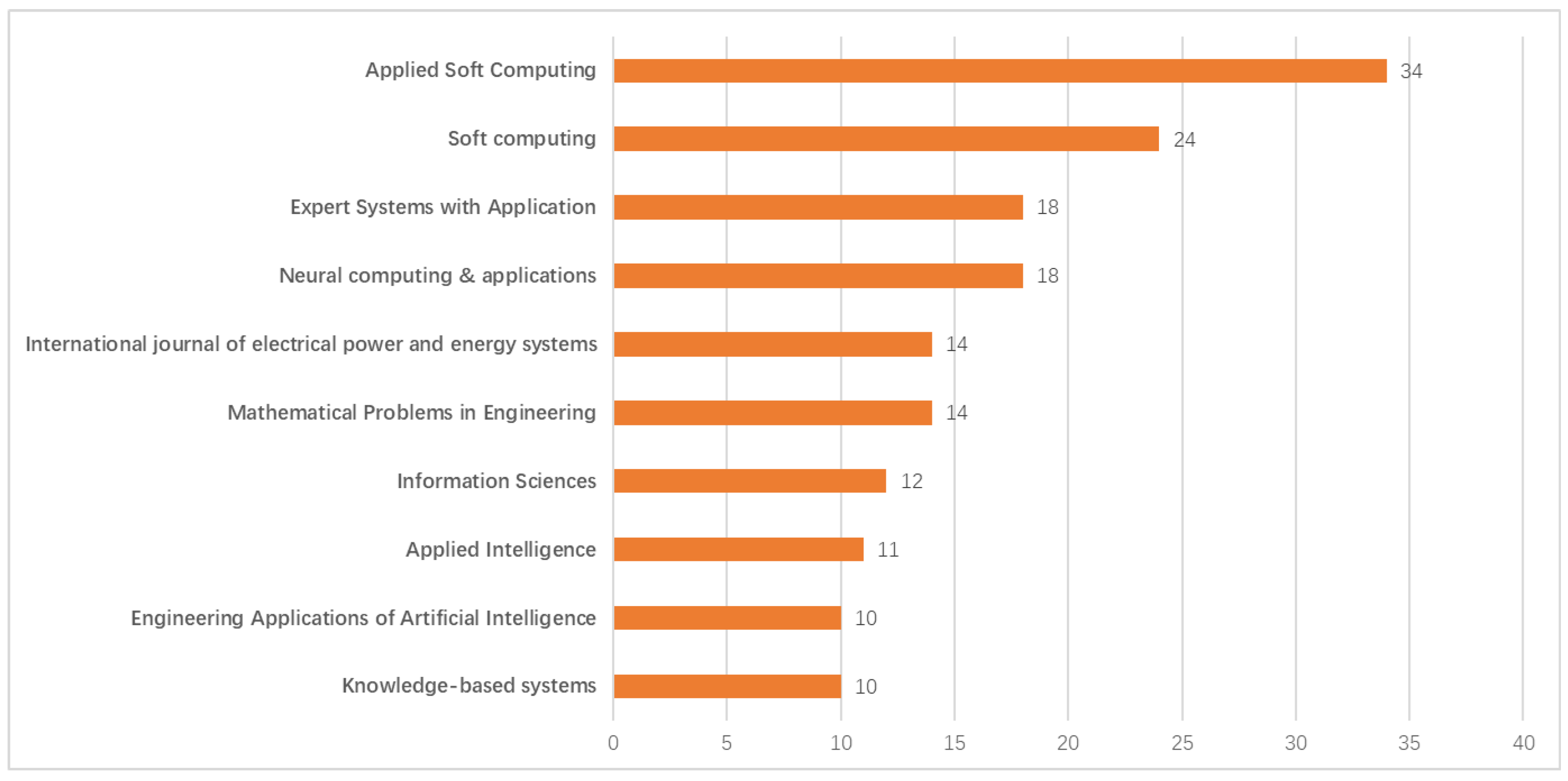
We investigated articles on the BBO algorithm in some well-known journals as shown in Figure 2. As you can see, BBO already exists in a certain number of variants, which makes its performance also improve. Unfortunately, these variants do not make the BBO algorithm suitable for high-dimensional optimization environments. BBO is still not effective in solving high-dimensional global optimization problems. Why not try to improve the BBO algorithm to solve them? Therefore, in order to make a breakthrough in this field, this paper proposes a simple and efficient multi-strategy-enhanced BBO variant based on the example chasing strategy, heuristic crossover strategy and prey search–attack strategy, referred to as MSBBO. It is “simple” because our algorithm has lower computational complexity, simpler steps and fewer parameters than BBO. It is “efficient” because our method can effectively solve large-scale global optimization problems up to 10,000 dimensions. The primary contributions of this paper are summarized as follows:
(1)
A novel framework of BBO is proposed, which is simpler and more efficient than the original BBO algorithm. Meanwhile, MSBBO has lower computational complexity than BBO.
(2)
MSBBO uses the example chasing strategy to eliminate the misguidance of bad information in the population. Then, the heuristic crossover and prey search–attack strategies are used to balance the exploration and exploitation of the population. MSBBO makes BBO suitable for high-dimensional optimization environments.
(3)
MSBBO successfully challenges the 10,000-dimensional numerical optimization problem. Compared with other meta-heuristic algorithms, its convergence performance is basically not affected by dimensions and has good ductility.
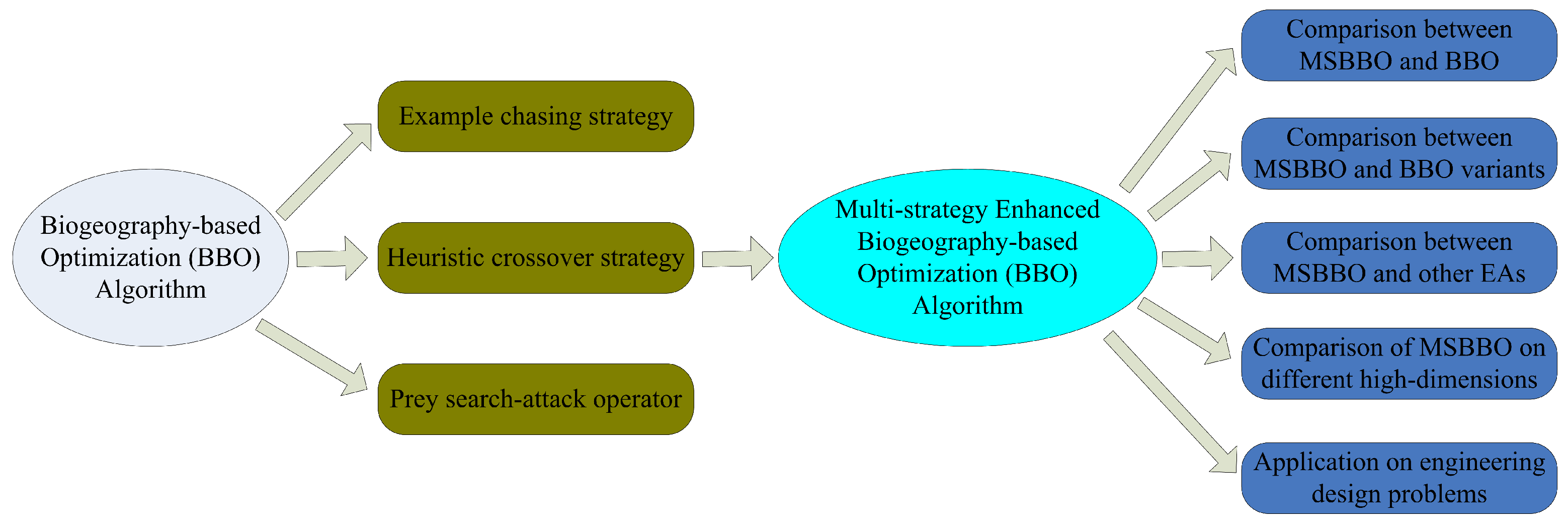
The organization of the rest of this paper is as follows: Section 2 introduces the standard BBO algorithm. Section 3 describes the three improvement strategies of MSBBO in this paper. Then, Section 4 analyzes the complexity of the proposed MSBBO. Section 5 is the numerical experiment and analysis. The last section, Section 6, is the conclusion. The graphical abstract of this paper is shown in Figure 3.

2. Standard BBO

In BBO, every habitat contains some characteristic variables. They determine how many species a habitat can hold and are called suitability index variables ( S I V s ). A habitat that is suitable for living species is interpreted as having a high habitat suitability index ( H S I ). So, the habitat with higher H S I is more likely to emigrate species, while the habitat with lower H S I is more likely to immigrate species. This is the main idea of BBO [15]. Table 1 shows the correspondence.
In the first stage, BBO uses Equation (1) to generate N habitats as the initial population, and each habitat contains D variables:
x i j = l b j + rand ( 0 , 1 ) · u b j l b j
where i = 1,2,…,N; j = 1,2,…,D. x i = ( x i 1 , x i 2 ,…, x i D ). u b j and l b j are the upper and lower limits of the j-th variable, respectively. Then, the  H S I of each habitat is calculated based on the fitness function, and the population is sorted by the H S I . Specifically, if  x i j is the best individual in the population, then i = 1 ; if x i j has the second highest fitness in the population, then i = 2 , and so on. In other words, the subscript i of x i j indicates its fitness ranking in the population. So, each x i is assigned a new i, and the species number S i of x i is calculated according to Equation (2):
S i = S m a x 2 · i , i = 1 , 2 , , N
where S m a x is the maximum species number, which is usually set to 2 · N . In this paper, we adopt the cosine migration model to calculate the immigration rate λ i and emigration rate  μ i :
λ i = I 2 1 + cos π · S i S m a x , μ i = E 2 1 cos π · S i S m a x .
where I is the maximum immigration rate and E is the maximum emigration rate. They are usually set to 1.
In the second stage, the specific operation of migration operator is to generate a random number between [0, 1] for each variable of x i . If it is smaller than λ i , in the remaining N-1 habitats, the  x k to be emigrated is determined according to μ k . Then, the variable of x k is used to replace the corresponding variable of x i .
In the third stage, it is the mutation operator. The species probability P i of each habitat is calculated through Equation (4):
P i = λ i + μ i P i + μ i + 1 P i + 1 , S i = 0 λ i + μ i P i + λ i 1 P i 1 + μ i + 1 P i + 1 , 1 S i S m a x 1 λ i + μ i P i + λ i 1 P i 1 , S i = S m a x
The mutation rate of a habitat is inversely proportional to its species probability. Therefore, the mutation rate m i of each habitat is as follows:
m i = 1 P i P m a x · m m a x , P m a x = m a x P i i = 1 N
where, m m a x is the maximum mutation rate. For each habitat x i , a number between [0, 1] is randomly generated, and if it is smaller than m i , x i needs to be mutated. Then, for each variable of x i , a random number in the range of upper and lower bounds is generated to replace the original variable. Algorithm 1 shows the computation pseudo-code of BBO.
Algorithm 1 Pseudo-code of the BBO.
initialize parameters: S m a x , I, E, N, and  m m a x
initialize the population by Equation (1)
for t = 1 to T do
   calculate the H S I and sort from best to worst
   calculate the S i by Equation (2), the  λ i and μ i by Equation (3)
   calculate the P i by Equation (4), the  m i by Equation (5)
   for i = 1 to N do
      % Migration
      for j = 1 to D do
         if rand(0,1) < λ i do
            select the x k according to { μ k } k = 1 N
            x i j = x k j
         end if
      end for
      % Mutation
      if rand(0,1) < m i do
         for j = 1 to D do
            x i j = l b j + rand ( 0 , 1 ) · u b j l b j
         end for
      end if
   end for
end for
output the optimal solution

3. Proposed Algorithm: MSBBO

3.1. Motivation

BBO uses roulette to select habitats to be emigrated, which can cause damage to the habitats with high H S I . At the same time, BBO replicates a single variable of another individual in the form of direct migration. However, a candidate solution performs well because the whole vector is closer to the optimal solution in the problem space, rather than because a single variable value performs well. In addition, the BBO random mutation operator cannot effectively help the algorithm to escape from the local optima. In fact, this mutation is blind and cannot maintain the population diversity. In addition, BBO relies only on the replacement of variables between different habitats to search for new solutions, which cannot balance the exploration and exploitation well and has a slow convergence speed. These are the main reasons why BBO cannot effectively solve high-dimensional numerical problems [38].
According to the literature reviews, we can observe that many studies have not completely overcome these shortcomings. Some variants change the mode of direct migration but do not eliminate the damage of inferior solutions to superior solutions, such as LxBBO [39], TDBBO [40], IWO/BBO [41], etc. Although HGBBO [42] and HFBBO [37] eliminate the damage of the inferior solutions to the superior solutions, the candidate solution changes only a certain part of variables in the migration. When solving high-dimensional optimization problems, the updating of candidate solutions cannot traverse every dimension. EMBBO [43] and NBBO [44] directly delete the random mutation operator but do not design more effective strategies to avoid the population falling into the local optima. In addition, the evolutionary mechanism of BBO itself determines that its performance ceiling is not high. Therefore, other heuristic strategies need to be considered to improve the convergence performance.
In view of the above shortcomings, this section proposes three improvement strategies to obtain a new variant of BBO with excellent performance. We firstly propose the example chasing strategy to eliminate the destruction of the inferior solutions to the superior solutions, thus effectively maintaining population diversity. Secondly, the heuristic crossover strategy is designed to enhance the search ability of the algorithm. The algorithm can search more adequately in the vicinity of superior individuals. Then, the prey search–attack strategy is designed to balance between the exploration and exploitation. In the evolution of the new algorithm population, the search emphasis is different in different stages. Meanwhile, to balance the computational complexity, the random mutation operator in the original BBO algorithm is deleted. The details are as follows.

3.2. Example Chasing Strategy

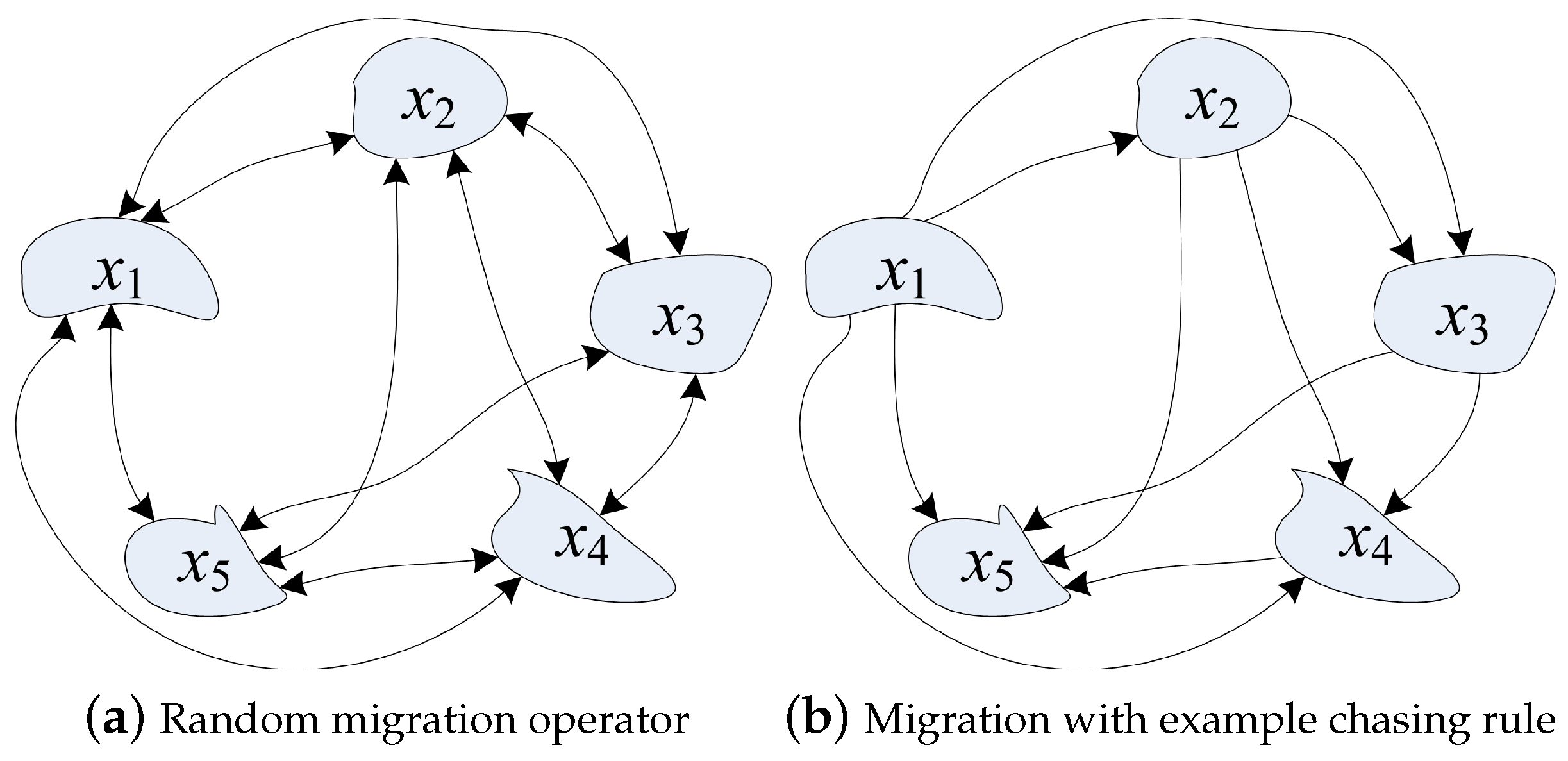
BBO randomly selects the candidate solution to emigrate, which is easy to damage the solutions with high fitness. For instance, x i is the immigration individual, and  x j is the emigration individual selected by roulette. There is a good chance that j is greater than i, which means that islands with lower H S I immigrate to islands with higher H S I , and the variables of the bad candidate solution replace the variables of the better one. It not only reduces the population diversity but also causes the population to deviate from the optimal solution. In fact, candidate solutions with high fitness tend not to accept variables from candidate solutions with low fitness. Therefore, to avoid the inferior individuals destroying the superior individuals, the example chasing strategy is designed. We set examples based on the ranking of each individual. For individual x i , it ranks i-th in the population, and the fitness of other individuals better than x i can only be x 1 , x 2 , . . . , x i 1 . These individuals rank higher than x i , so they become the examples of x i , and  x i becomes the chaser. Everyone has a natural tendency to chase the examples, so the chasers achieve better fitness by chasing their examples. The reason why human beings can progress is they continue to learn from the best and surpass them. To intuitively explain the principle of the example chasing strategy, Figure 4 is plotted.
As shown in Figure 4a, every two-candidate solution can migrate to each other. x 1 can be replaced by any lower-fitness solution, while x 5 can emigrate variable values to any better candidate solution. So, random migration will cause the inferior individuals to destroy the superior individuals, thus reducing the population diversity. Figure 4b is the example chasing strategy. It can be observed that only unidirectional migration can be carried out between candidate solutions. That is, the poor individuals can only accept features from the better individuals, and the poor individuals cannot affect the better individuals. For instance, only x 1 is ranked higher than x 2 , so x 2 can only accept the variables from x 1 , while individuals ranked lower than x 2 can accept the variables from x 2 but cannot emigrate to it.
During the migration of x i , the example x k of x i can be selected by Equation (6):
k = r o u n d ( c e i l ( 1 , i 1 ) ) , i = 2 , 3 , , N .
where c e i l ( ) is a random number between 1 and i, and r o u n d ( ) is an integer function.
Therefore, the example chasing strategy avoids the bad influence of poor individuals on good individuals, effectively maintains the population diversity, and speeds up the search of the population to the optimal solution. In addition, it does not need to calculate the emigration rate of each individual, which reduces the calculation amount.

3.3. Heuristic Crossover Strategy

In the natural evolution of organisms, two homologous chromosomes through mating and recombination will form a new chromosome, thus giving rise to a new individual or species [45]. New individuals often absorb the advantages from their parents and thus better adapt to the current living environment. If it is used in the evolutionary algorithm, the search efficiency of the population in the search space can be improved. Inspired by this idea, to overcome the defects of the direct migration mode in the BBO algorithm, this paper designs a dynamic random heuristic crossover strategy as shown in Equation (7):
x i t + 1 = x k t + α ( x b e s t t x i t )
where t is the current iteration number, k is the example individual selected by Equation (6), and  x b e s t t is the optimal individual of the current population. It should be noted that the heuristic crossover we designed is carried out for the whole candidate solution vector, rather than including only some variables like the standard BBO algorithm. Therefore, when solving a high-dimensional global optimization problem, the search of the problem space for candidate solutions can traverse every dimension.
Equation (7) has an important impact on the performance of MSBBO, and is expected to improve the search ability and convergence speed of MSBBO in the iterative process. It consists of a basis vector and a difference vector. The former is used to determine the search center, and the latter is used to control the search scope and direction. In the MSBBO framework, to make full use of the promising information provided by elite individuals and their guiding effect on other individuals, we use example individuals as the base vector. We have reason to believe the better solution is closer to the optimal solution, so the population can search in more valuable areas. The role of examples is crucial to the growth of an individual. It is because we have role models that we can become better people. We enhance our own abilities by mimicking the behaviors of examples or by being influenced by their personalities. Poor candidate solutions can also improve their competitiveness by absorbing the characteristics of good solutions. In addition, the optimal solution x b e s t t of the current population is used to generate the difference vector to ensure a preferable searching direction. Through this strategy, individuals can exploit the area around an example; meanwhile, they can be attracted by the x b e s t t .
The dynamic parameter α is a random number that varies nonlinearly with the current iteration number t, which is given as Equation (8):
α = 1 2 sin ( 2 π f r e q t ) t T + 1
The main idea of the dynamic parameter α is to design a novel formula which not only permits the adjustment of parameter values but also permits the adjustment of its direction. Such a possibility is well offered by the sine function. By transforming the sine function, the value of a given parameter increases and decreases periodically. This is accurately what we need, with some flexibility in the search direction when changing the parameter. f r e q is used to control the fluctuation frequency of parameter α . After a lot of experiments, we suggest that the best value of f r e q is 0.25.

3.4. Prey Search–Attack Operator

The BBO random mutation operator easily generates low-quality habitats and reduces the population diversity. It cannot effectively help the algorithm to escape from the local optima, and the calculation of species probability consumes much CPU time. Therefore, in MSBBO, we delete the random mutation operator, which further reduces the computational complexity. Meanwhile, inspired by the searching and attacking behavior of predators [46], we put forward the prey search–attack operator. It supposes the best solution of the current population x b e s t t is the prey p t , and the rest N-1 solutions are predators. Then, the searching and attacking behavior is defined as the following:
p t = ω 1 · x i t + ω 2 · x b e s t t x i t
x i t + 1 = | x b e s t t p t |
Equation (9) is used for searching the prey x b e s t t , and Equation (10) is used for attacking the prey x b e s t t . ω 1 and ω 2 are two self-adjusting parameters, which can be calculated by the following:
ω 1 = ( r a n d + 1 ) · ( 1 t / T )
ω 2 = 2 · ( 1 t / T ) · ( r a n d 0.5 )
where ω 1 and ω 2 are used to better balance between the exploration and exploitation over the whole evolution. The former is responsible for the global search, that is, exploration; the latter is responsible for the local search, that is, exploitation. ω 1 makes x i search spaciously in the entire solution space where the prey x b e s t t lives. On the contrary, ω 2 makes x i search around a small limited small area of the prey x b e s t t . The values of ω 1 and ω 2 are both large at the beginning of the evolution because in the early stage, it is necessary to maintain the population diversity. Later in the iteration, the population has already closed to the optimal solution, and it is not recommended to search in a large range. Instead, a more refined exploit should be tried near the optimal solution, so the values of ω 1 and ω 2 are all small. Therefore, the parameters ω 1 and ω 2 guarantee a dynamic balance of the exploration and exploitation.
To sum up, this section proposes a multi-strategy enhanced BBO variant based on the example chasing strategy, heuristic crossover strategy and prey search–attack operator. Algorithm 2 shows the calculation flow of MSBBO.
Algorithm 2 Pseudo-code of the MSBBO.
initialize parameters: S m a x , I , N , f r e q
initialize the population by Equation (1)
calculate the S i by Equation (2), the  λ i by Equation (3)
calculate the HSI and sort from best to worst
for t = 1 to T do
   for i = 1 to N do
      if rand(0,1) < λ i do
         select the x k according to Equation (6)
         heuristic crossover of x i by Equations (7) and (8)
      end if
      calculate the ω 1 by Equation (11), the  ω 2 by Equation (12)
      search the prey by Equation (9)
      attack the prey by Equation (10)
   end for
   calculate the HSI and sort from best to worst
end for
output the optimal solution

4. Complexity Analysis

In this section, the computational complexity of MSBBO and BBO is compared. The comparison between Algorithms 1 and 2 shows that MSBBO moves the calculation of the immigration rate out of the loop. Because it is based on the ranking, there is no need to calculate again. In BBO, the N individuals’ immigration rate and emigrate rate are calculated in each iteration. So, the total calculation complexity of BBO is O ( 2 · T · N ) . While MSBBO adopts the example chasing strategy to select the emigration individual, there is no need to calculate the emigration rate, so the calculation time is O ( N ) . The original migration operator of BBO requires each dimension of each individual to be judged and computed separately, so the total computation is O ( T · N · D ) . While the heuristic crossover of MSBBO migrates the whole candidate solution vector and reduces one “for” loop, the computational complexity is O ( T · N ) . Then, in the mutation operator, according to Equations (4) and (5), its calculation times of each generation are O ( 2 · N ) . So the total calculation times of the BBO mutation operator is at least O ( 2 · T · N ) . MSBBO uses prey search–attack operator to replace the mutation operator, which adds two calculation times in each iteration. So, the total calculation complexity is also O ( 2 · T · N ) . However, MSBBO has fewer judgments than BBO in each iteration because the execution of the prey search–attack operator does not need to generate random numbers for judgment. So, BBO has O ( T · N ) more computation times than MSBBO in generating random numbers.
According to the above analysis, the computational complexity of BBO is O ( T · N ( D + 5 ) ) , while that of MSBBO is O ( N ( 3 · T + 1 ) ) . The MSBBO designed in this paper can effectively reduce the calculation cost of the BBO algorithm and reduce the calculation amount. We will further verify this by experiments later on.

5. Experimental Results and Analysis

5.1. Experiment Preparation

In order to fully test the comprehensive performance and competitiveness of MSBBO, in this section, a series of comparative experiments are made on a set of classic benchmark functions and several engineering design optimization problems. We first compare the MSBBO algorithm with the standard BBO algorithm to verify the effectiveness of the three improvement strategies. We then compare MSBBO to seven excellent BBO variants to verify the superiority of MSBBO in the same class of algorithms. After that, in order to verify the advancement of MSBBO in different algorithms, we choose seven new meta-heuristic algorithms to compare with it. Finally, we apply the proposed algorithm to six practical engineering problems, and select five advanced optimization techniques as competitors to demonstrate the value and development potential of MSBBO at the application level. The used well-known benchmark functions are shown in Table 2. They contain complex problems such as unimodal, multimodal, irregular, compound and nonlinear, which can fully test the comprehensive performance of the algorithms. The number of independent runs is 51, and the population size (N) of each compared algorithm is 50. We choose the Wilcoxon rank-sum test to analyze and evaluate all experimental results [47]. Then, the development environment is MATLAB R2022a.

5.2. Comparison between MSBBO and Standard BBO

In order to test the effectiveness of MSBBO, we compare MSBBO with BBO first in this subsection. The standard BBO is not suitable for large-scale optimization problems, so we compare the performance of the two algorithms on 30, 50 and 100 dimensions, respectively. Our work does not add additional function evaluations, that is, the maximum iteration number (T) of MSBBO should be equal to that of BBO. We set T = 1000 . The mean and standard deviation of the 51 errors are summarized in Table 3, and the last line is the results of the Wilcoxon rank-sum test. The representative meaning of “(w/t/l)” is w(+: win)/t(≈: tie)/l(-: lose), where “-” means that the performance of the compared algorithm is worse than MSBBO, “+” means the compared algorithm is superior, and “≈” means the compared algorithm is similar to MSBBO. The bolded data represents the best value in both algorithms.
It can be seen from Table 3 that the numerical calculation results of the proposed MSBBO algorithm on 24 benchmark functions (D = 30, 50 and 100) are significantly better than those of the BBO algorithm. This shows that our work has obviously improved the convergence accuracy of BBO. Through careful observation, it can be seen that the results of MSBBO on 30, 50 and 100 dimensions are basically the same, indicating that its performance is almost unaffected by dimensional changes on the lower dimensions. According to this, MSBBO has good malleability and can challenge higher dimensions. When D = 100 , MSBBO also converges to the optimal value with zero error on 20 benchmark functions. This shows that MSBBO acquires a better exploration ability and still preserves the exploitation ability. This is because the example chasing strategy proposed in this paper blocks the transmission of bad information of the inferior solutions to the superior solutions, thus successfully maintaining the population diversity. The heuristic crossover strategy can enhance the random search ability of the algorithm. It helps the population exploit more fully in the vicinity of a superior candidate solution, thereby efficiently improving the convergence accuracy. At the same time, the prey search–attack operator helps the population to switch freely between global search and local search so as to quickly find the optimal evolutionary direction. Therefore, the improvement strategies in this paper effectively enhance the overall performance of the original BBO algorithm so that it can achieve the balance between exploration and exploitation. The three strategies complement each other, without excess, and work together.
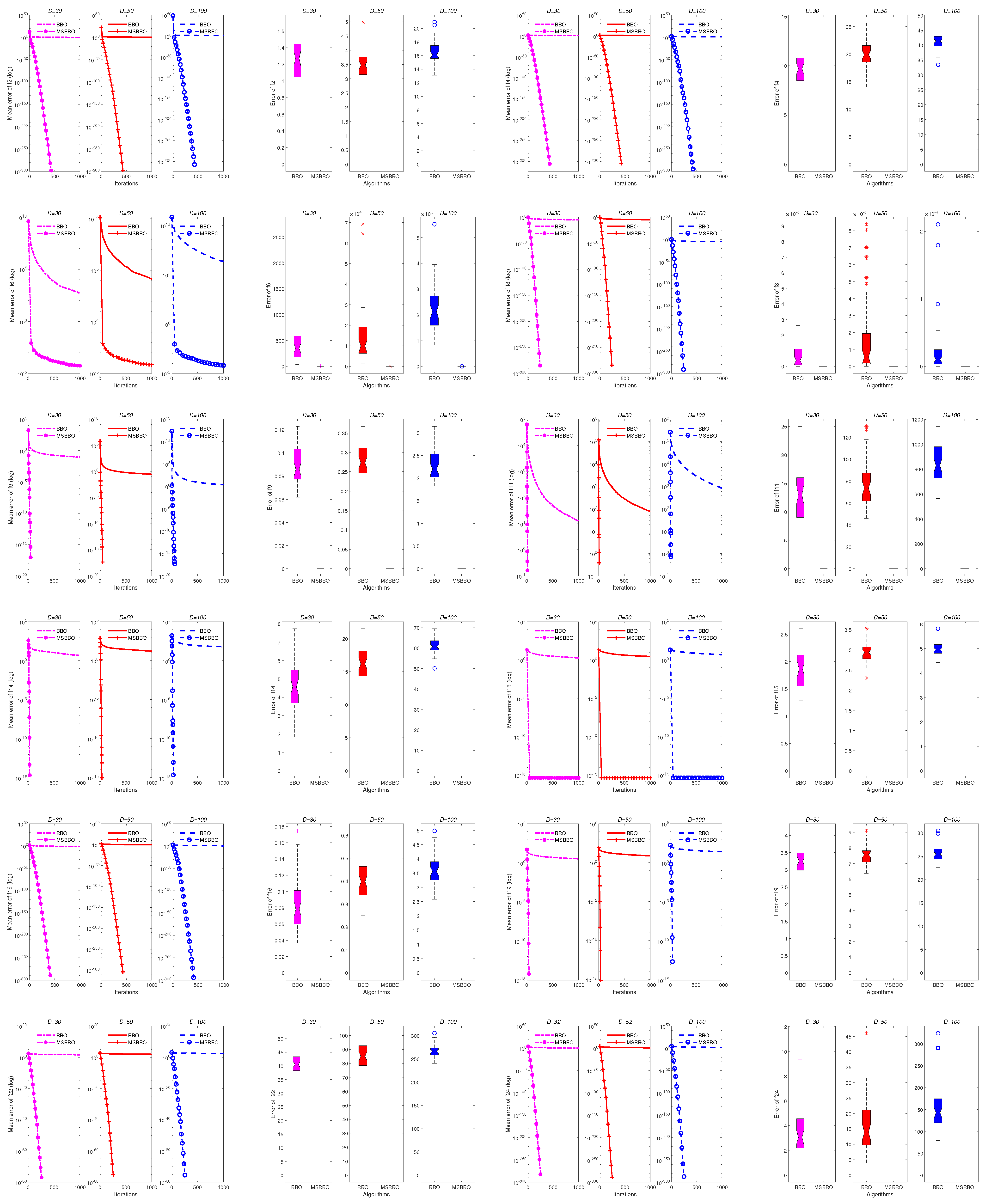
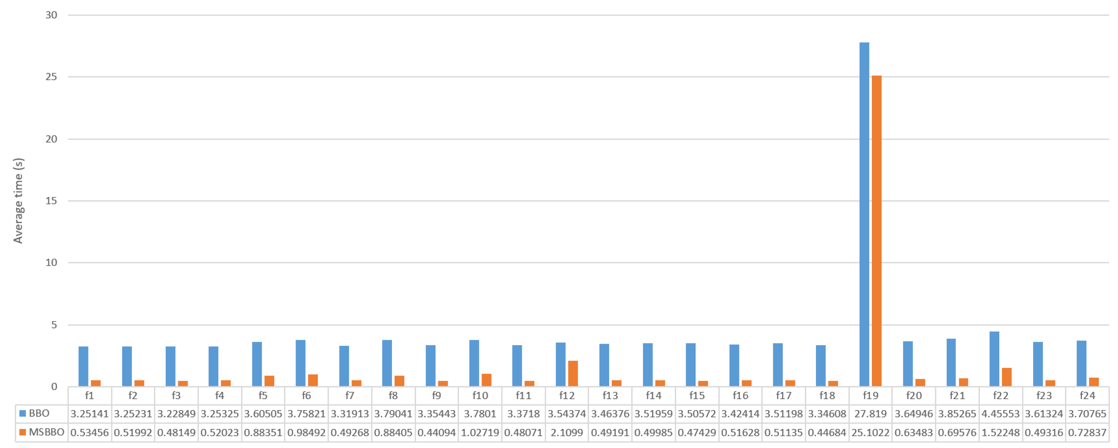
Then, to provide an intuitive comparison [48,49], some convergence curves and boxplots of MSBBO and BBO are plotted as shown in Figure 5. The convergence curve is used to observe the convergence rate and the evolution state of the population, and the boxplot is used to evaluate the stability of the algorithm. From Figure 5, MSBBO converges much faster than BBO on all selected functions (D = 30, 50 and 100). Especially on the functions f 9 , f 11 , f 14 and f 19 , the convergence curve of MSBBO decreases rapidly, which indicates that its population is rapidly concentrated towards the optimal solution. This shows that the strategies in our work can accelerate the convergence speed of the original algorithm by a large margin. Further, all the convergence trends of MSBBO on the three low-dimensions are basically the same, and there is no obvious difference. This also proves that the convergence performance of the proposed approach is not affected by dimensional changes on low dimensions. Meanwhile, by carefully observing the boxplots, it also shows that MSBBO is more stable and has stronger robustness than BBO. The results of 51 runs of the BBO algorithm fluctuate greatly, and there are outliers, such as functions f 2 , f 6 , f 8 and f 24 , etc. MSBBO does not have any outliers, and the boxplot on all functions is almost a straight line. This means that each search of MSBBO converges to almost the same optimal value, providing superior consistency. In addition, both BBO and MSBBO were run 51 times on each benchmark function ( D = 100 ), so we calculated their respective average run times on each function as shown in Figure 6. It can be intuitively found that the average calculation time of MSBBO on each function is much smaller than that of BBO, which not only improves the convergence accuracy but also saves time consumption. It also verifies that the complexity analysis in Section 4 is correct, and MSBBO has a simpler framework that reduces the unnecessary calculation of the immigration rate and the judgment steps for each dimension.
According to the above experiments and discussions, the performance of MSBBO is fully better than that of BBO. Therefore, the improvement strategies in our work successfully enhance the optimization capacity of BBO. In particular, MSBBO improves the malleability of the algorithm to the problem dimension.

5.3. Comparison between MSBBO and BBO Variants

In this subsection, we compare MSBBO with seven excellent BBO variants: PRBBO [50], BBOSB [51], HGBBO [42], FABBO [52], BLEHO [53], MPBBO [54] and BBOIMAM [55]. We compare their performance on 200 dimensions. Consistent with Section 5.2, eight algorithms search the optimal values on 24 benchmark functions, and the mean and standard deviation of 51 errors are used as evaluation indexes. Table 4 shows the comparison results. Among them, the mean error is the focus of comparison, and the bold data represent the optimal value.
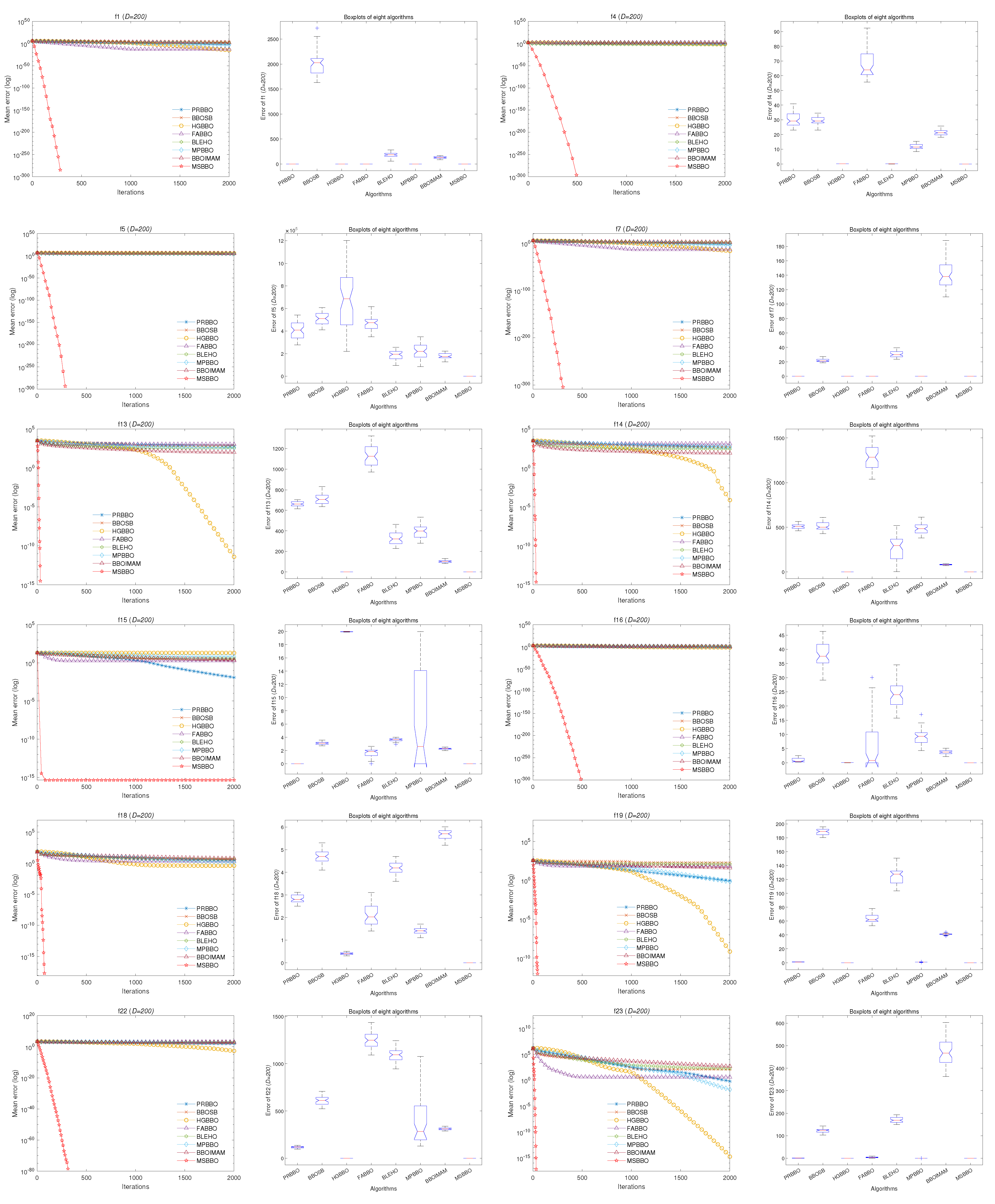
From Table 4, MSBBO outperforms all BBO variants more than 90% of the problems according to the Wilcoxon rank-sum test. The experimental results of PRBBO and HGBBO are the same, their convergence results on f 20 and f 21 are better than MSBBO, and they converge to the same optimal value on f11, but the convergence results on the remaining 22 functions are worse than MSBBO. BBOSB performs better than MSBBO only on f 21 and worse on all other functions. In contrast, FABBO is the least competitive, with significantly worse experimental results than MSBBO on all functions. In the high-dimensional environment of 200 dimensions, MSBBO can still converge to the theoretical optimal value on 20 benchmark functions, which is basically consistent with the results in Table 3. This shows that the performance of the MSBBO algorithm does not decrease significantly with the increase in dimension, and can adapt well to the high-dimensional optimization environment. In addition, MSBBO performs better on 91.7% of the benchmark problems than other algorithms of the same class, demonstrating the superiority of this paper’s work in the BBO variants. It achieves more trustworthy results with a simpler algorithmic structure and complexity. Also, for better evaluation, the convergence curves and boxplots of them on different functions are shown in Figure 7. Obviously, MSBBO converges the fastest on all functions and does not fall into local optima. Especially on functions f 13 , f 14 , f 19 and f 23 , the convergence curves of MSBBO are almost perpendicular to the horizontal axis; the convergence speed is fast. The example chasing strategy prevents population degradation, so the convergence curves of MSBBO will not fluctuate and will always converge. Then, the heuristic crossover strategy ensures that the population search can traverse every dimension, so MSBBO can quickly find the evolutionary direction in high-dimensional environments. Finally, the prey search–attack strategy ensures the dynamic balance between global exploration and local exploitation of the population, and successfully improves the convergence rate. In addition, a closer look at the boxplots shows that MSBBO has almost no boxplot and no outliers on all benchmark functions. In contrast, other BBO variants have erratic performance on some functions, and their algorithmic generality is relatively low. Therefore, the improvement strategies designed in this paper effectively improve the comprehensive performance of the original algorithm and have strong competitiveness among BBO variants.
To sum up, the performance of MSBBO is better than that of PRBBO, BBOSB, HGBBO, FABBO, BLEHO, MPBBO and BBOIMAM. Compared to the same type of algorithm, MSBBO has outstanding ductility and is more suitable for high-dimensional optimization problems.

5.4. Comparison between MSBBO and Other Meta-Heuristic Algorithms

To further verify the superiority of MSBBO for solving large-scale optimization problems, we compare it with seven meta-heuristic algorithms proposed in the past few years: GWO [56], WOA [13], SSA [57], ChOA [58], MPA [59], GJO [60] and BWO [61]. Among them, GWO, WOA, SSA, ChOA and MPA are highly cited algorithms. GJO and BWO are the novel algorithms proposed in the last years which are competitive. Therefore, MSBBO can further verify its advancement by comparing with these outstanding algorithms. We compare their performance on 500 dimensions. Similarly, the mean and standard deviation of 51 errors are used as evaluation indexes. Table 5 shows the experimental results, and the bold data represent the optimal value.
According to Table 5, MSBBO still has the best overall performance among the eight new meta-heuristic algorithms, with the minimum mean error obtained on 22 functions and zero error on 20 functions. GWO converges to the theoretical optimal value on three functions ( f 11 , f 13 and f 23 ), while the results on the remaining 21 functions are inferior to MSBBO. WOA converges to the theoretical optimal value only on the function f 9 , and the experimental results on the remaining functions are inferior to MSBBO. SSA and BWO converge to relatively better results among the eight compared algorithms on f 20 and f 21 , the results on f 11 are equal to MSBBO, and the results on the other functions are inferior to MSBBO. However, ChOA and GJO do not show some competitiveness, and the experimental results on 24 benchmark functions are inferior to MSBBO. In contrast, SSA and MPA are more competitive. MPA outperforms MSBBO on two functions ( f 20 and f 21 ) and converges to the optimal solution on eight functions ( f 8 , f 9 , f 11 , f 13 , f 14 , f 17 , f 19 and f 23 ). Although these novel algorithms show excellent performance on low-dimensional problems, their precision obviously decreases when solving high-dimensional optimization problems. On the contrary, even when D = 500 , MSBBO converges error-free to the optimal value of the objective function on 20 problems. In other words, our work is still clearly competitive among different types of meta-heuristic algorithms, so it is advanced. A careful comparison between Table 4 and Table 5 shows that the experimental results of MSBBO on 200 dimensions are almost the same as on 500 dimensions. Therefore, the improvement strategies in our work enable the population to search in a high-dimensional environment, and the algorithm performance has good ductility.
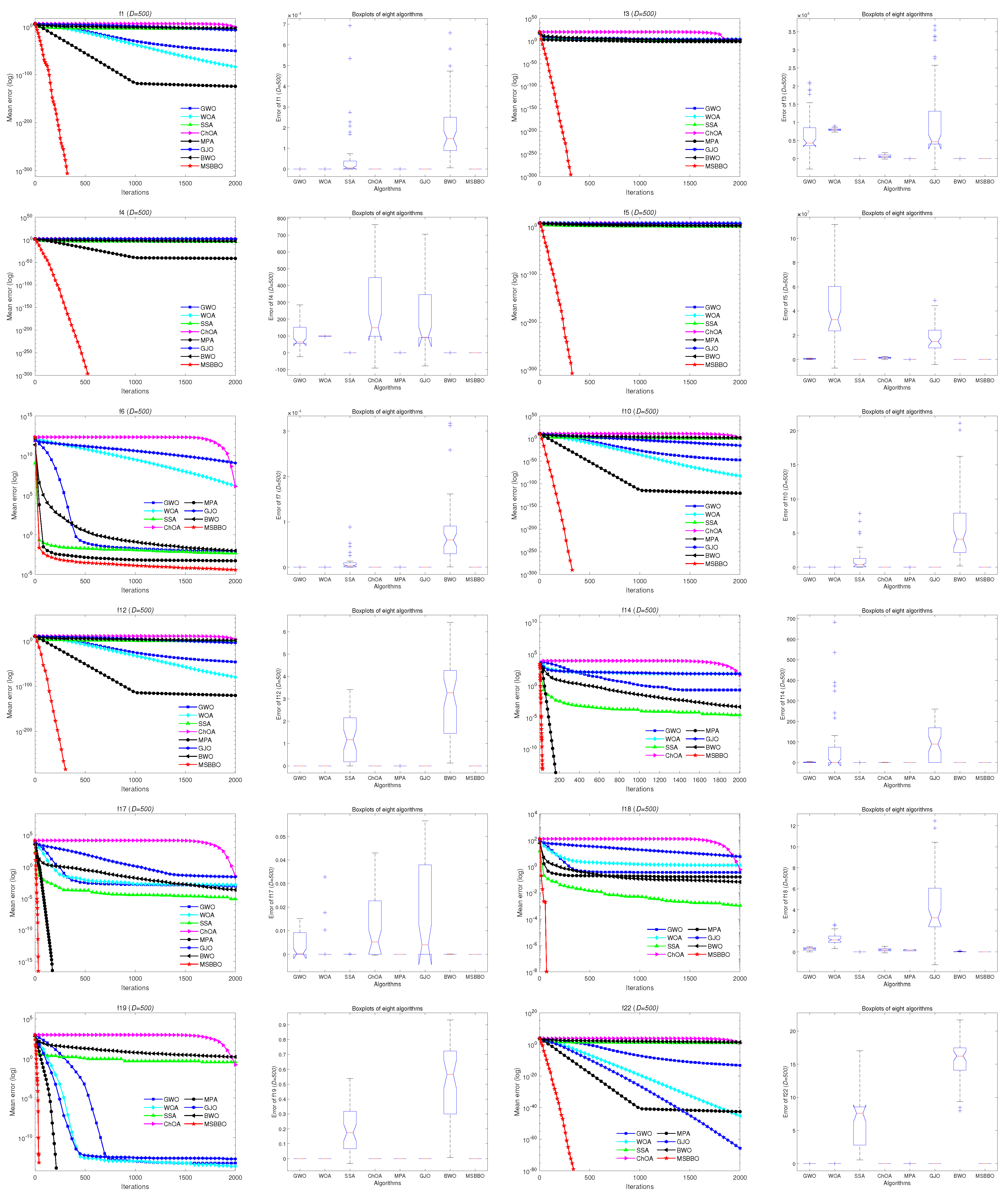
For a better evaluation of MSBBO and the seven new meta-heuristic algorithms, Figure 8 shows the convergence curves and boxplots of them on different problems. It can be found that the MSBBO algorithm converges much faster than other competitors on different benchmark functions, saving at least 1500 iterations and not falling into the local optima. Especially on functions f 13 , f 14 , f 15 , f 19 and f 23 , MSBBO converges rapidly, and the convergence curve is almost invisible. Further, even if D = 500 , the boxplot of MSBBO on different functions is almost invisible, and the algorithm performance remains stable. This shows that MSBBO can continue to challenge higher-dimensional problems.
According to the above analysis, for large-scale optimization problems, the performance of MSBBO is significantly better than that of GWO, WOA, SSA, ChOA, MPA, GJO and BWO in both solution quality and convergence speed. In addition, the convergence performance of MSBBO on 500 dimensions is not overtly different from that on low dimensions, so the performance is maintained well.

5.5. Comparison of MSBBO on Different High Dimensions

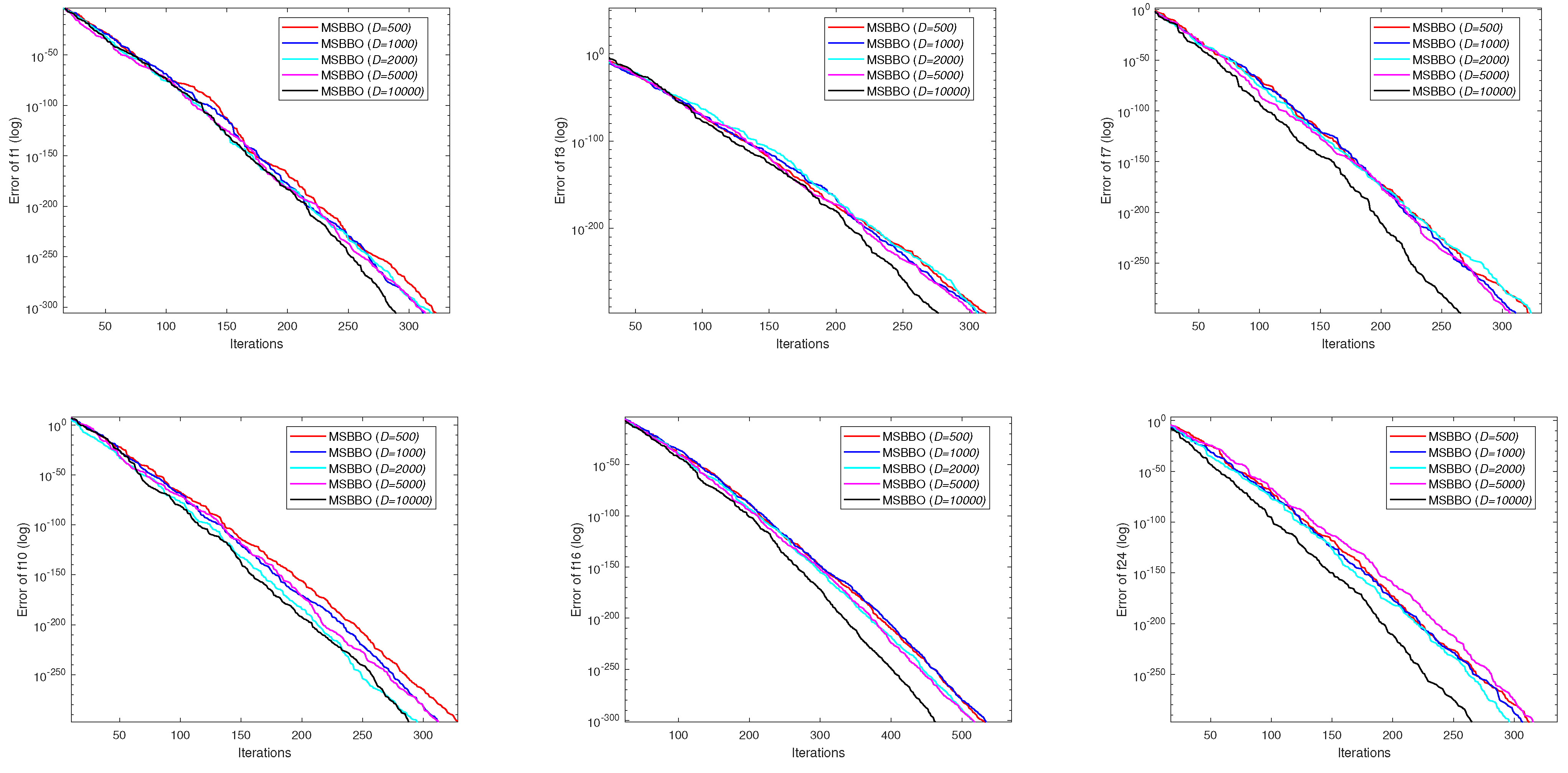
Although problems with more than 100 dimensions are defined as high-dimensional optimization problems. But in fact, many large-scale optimization problems in human society go far beyond 100 dimensions, and even beyond thousands of dimensions. In this context, the ability of the algorithm to adapt to high-dimensional optimization environment needs to be as strong as possible. In order to conduct a more thorough examination and testing, we compare the performance of MSBBO on the dimensions of 500, 1000, 2000, 5000 and 10,000, respectively. The mean error and standard deviation of the results are summarized in Table 6. As shown in Table 6, except for f 20 and f 21 , MSBBO basically converges to the same results on 10,000 dimensions as on 500 dimensions. Though the accuracy is reduced on f 6 , it does not exceed two exponential levels. Therefore, in the search space below 10,000 dimensions, the convergence accuracy of MSBBO is basically not affected by the dimensions. Then, to fully demonstrate the advantages of MSBBO in high-dimensional environments, some convergence curves of MSBBO on different dimensions are plotted and shown in Figure 9.
From Figure 9, it is not difficult to conclude that with the increase in dimensions, the convergence curves of MSBBO are basically the same. There is no obvious separation of the convergence curves on different dimensions. In other words, there is basically no difference in the domain structure of populations on different dimensions, and they can also gather quickly in a high-dimensional space. The performance of most meta-heuristic algorithms decreases significantly with the increase in dimension, but the performance of MSBBO is relatively little affected by the change of dimension. It is fair to say that we have taken on a very challenging job, as there are very few algorithms that can plot the effects of Figure 9. Our algorithm has great advantages in solving high-dimensional optimization problems.

5.6. Application on Engineering Design Problems

Finally, we are also concerned about the application value of MSBBO in practical problems. To simply verify the usefulness of MSBBO, we apply it to the following six real-world engineering optimization problems: pressure vessel design, tension/compression spring design, welded beam design, speed reducer design, step-cone pulley problem and robot gripper problem. At the same time, these problems are also solved by some new advanced optimization techniques. Therefore, we selected six optimization methods (COA [62], EDO [63], OMA [64], SHO [65] and SCSO [66]) just proposed in 2023 to compare the results to fully verify the superiority and competitiveness of MSBBO. The population size of all algorithms is 50, and the maximum number of iterations is 1000.
The six engineering design problems are all constrained optimization problems. When using meta-heuristic algorithms to solve constraint optimization problems, besides the performance of the algorithm, the processing technology of constraint conditions is also very important. If the treatment of constraints is not applicable, even the algorithm with superior performance cannot search for the optimal solution. In order to make the six engineering problems meet the use conditions of the meta-heuristic algorithm and the experimental results more dependent on the search ability of the algorithm, we choose the penalty function method in literature [67] to deal with the constraints of these problems:
Minimize F ( x ) = f ( x ) ± i = 1 p a i G i ( x ) + j = 1 q b j H j ( x ) G i ( x ) = max 0 , g i ( x ) η H j ( x ) = h j ( x ) λ
G i ( x ) is the inequality constraint, H j ( x ) is the equality constraint, p is the number of inequality constraints, q is the number of equality constraints, a i and b j are constant, η and λ is equal to 1 or 2. For this penalty method, when the candidate solution violates any constraint, the value of the objective function increases, pushing the population into the feasible region from the infeasible solution [67].

5.6.1. Pressure Vessel Design

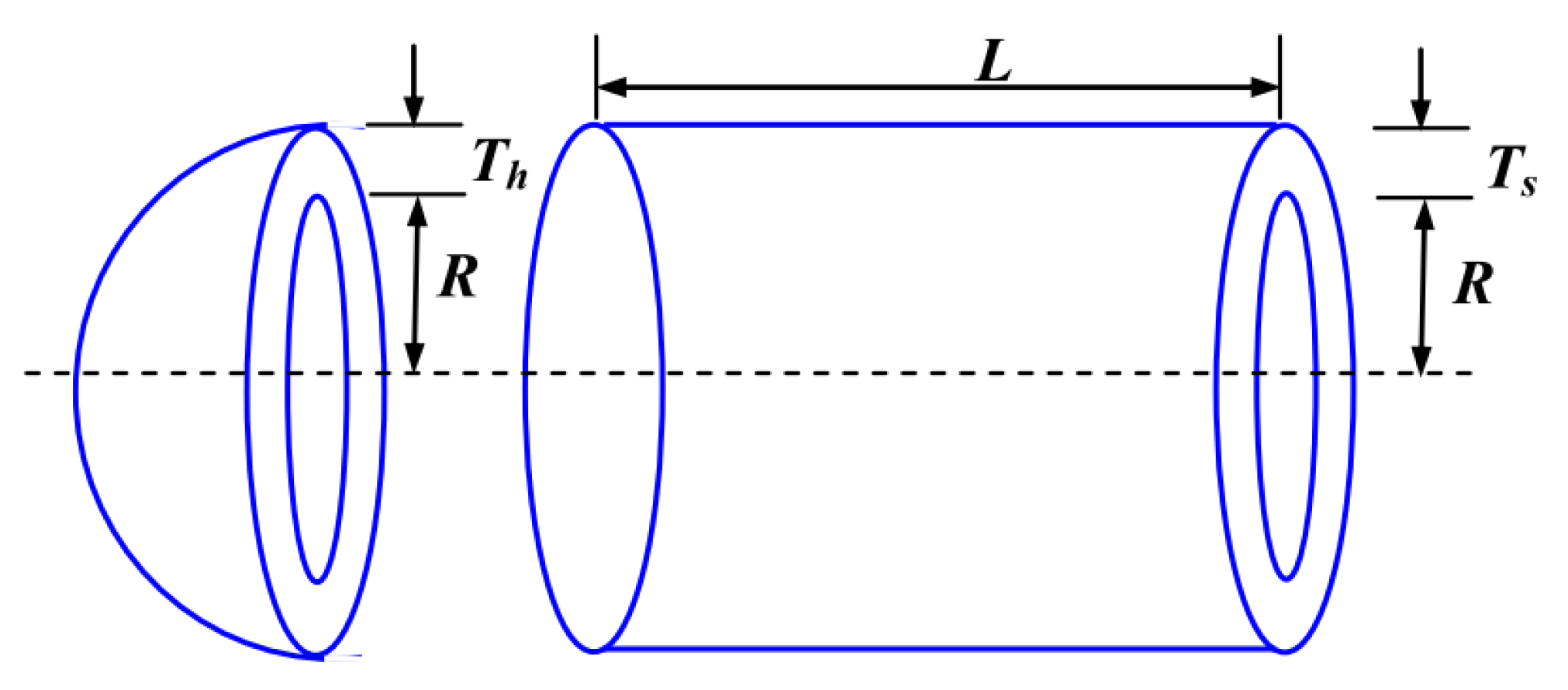
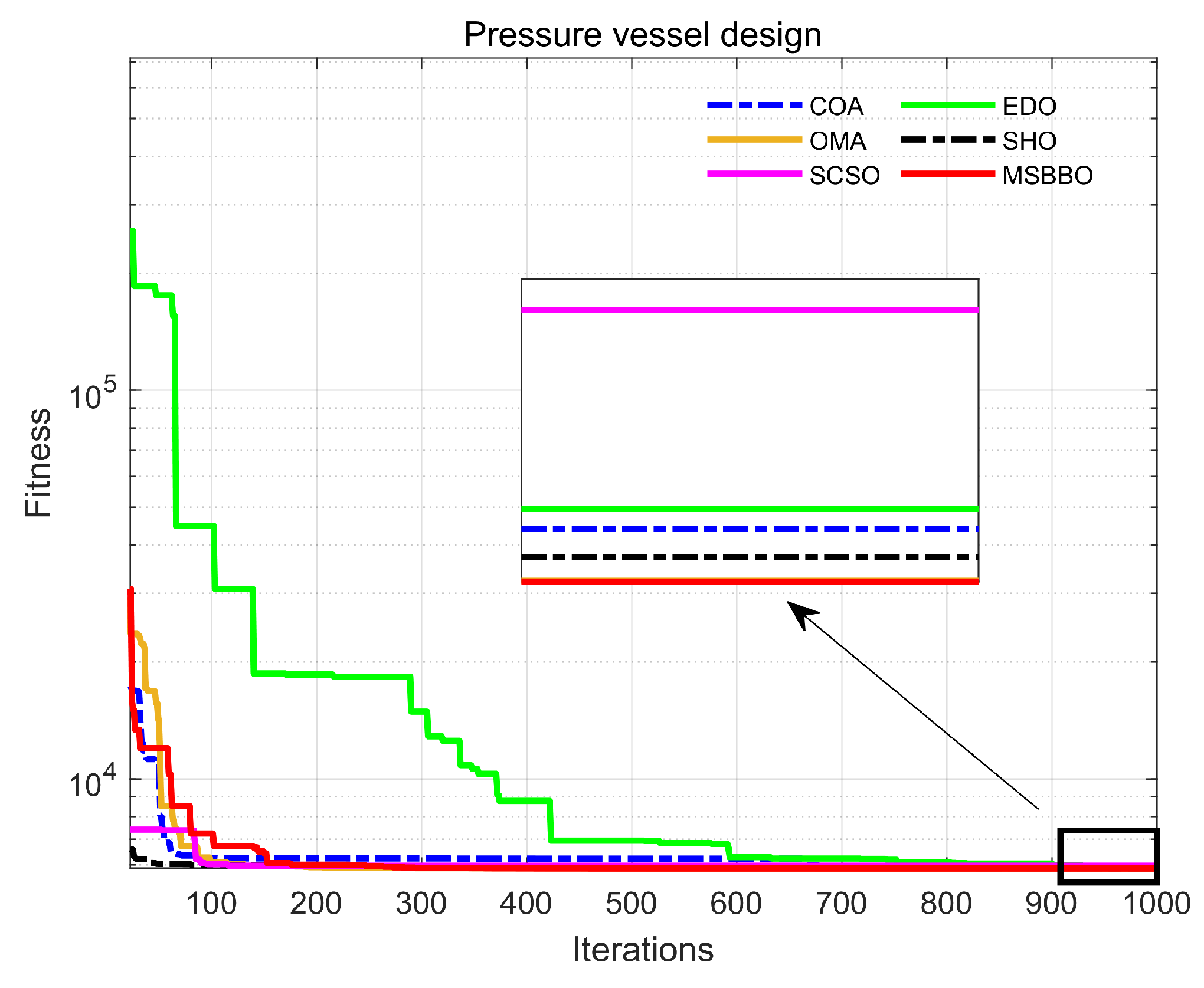
The goal of the pressure vessel design problem is to minimize the cost of fabrication [68]. As shown in Figure 10, L is the section length of the cylinder part without considering the head, R is the inner wall radius of the cylinder part, T s and T h are the wall thicknesses of the cylinder part and the head, respectively [68]. Therefore, T s , T h , R and L are the four optimization variables. The mathematical formulation and four constraint functions are shown in Equation (14). The optimal results of the six comparison algorithms are summarized in Table 7, and the convergence curves of the objective function on this problem are shown in Figure 11.
X = x 1 , x 2 , x 3 , x 4 = T s , T h , R , L minimize f ( X ) = 0.6224 x 1 x 3 x 4 + 1.7781 x 2 x 3 2 + 3.1661 x 1 2 x 4 + 19.84 x 1 2 x 3 s . t . g 1 ( X ) = x 1 + 0.0193 x 3 0 g 2 ( X ) = x 2 + 0.00954 x 3 0 g 3 ( X ) = π x 3 2 x 4 4 π x 3 3 / 3 + 1296000 0 g 4 ( X ) = x 4 240 0 where 0 x i 100 , i = 1 , 2 ; 10 x i 200 , i = 3 , 4
As can be seen from Table 7 and Figure 11, our work achieves a smaller objective function value (5885.33277894) than the other five new technologies, which further optimizes the pressure vessel design problem. Under the condition of satisfying various constraints, MSBBO gives a new and better solution: [ T s , T h , R, L] = [0.77816864, 0.38464916, 40.31961873, 200].

5.6.2. Tension/Compression Spring Design

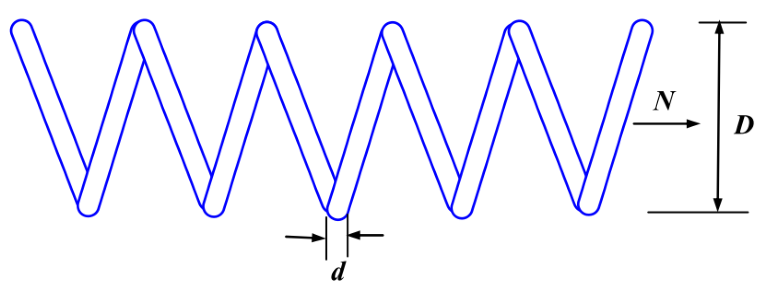
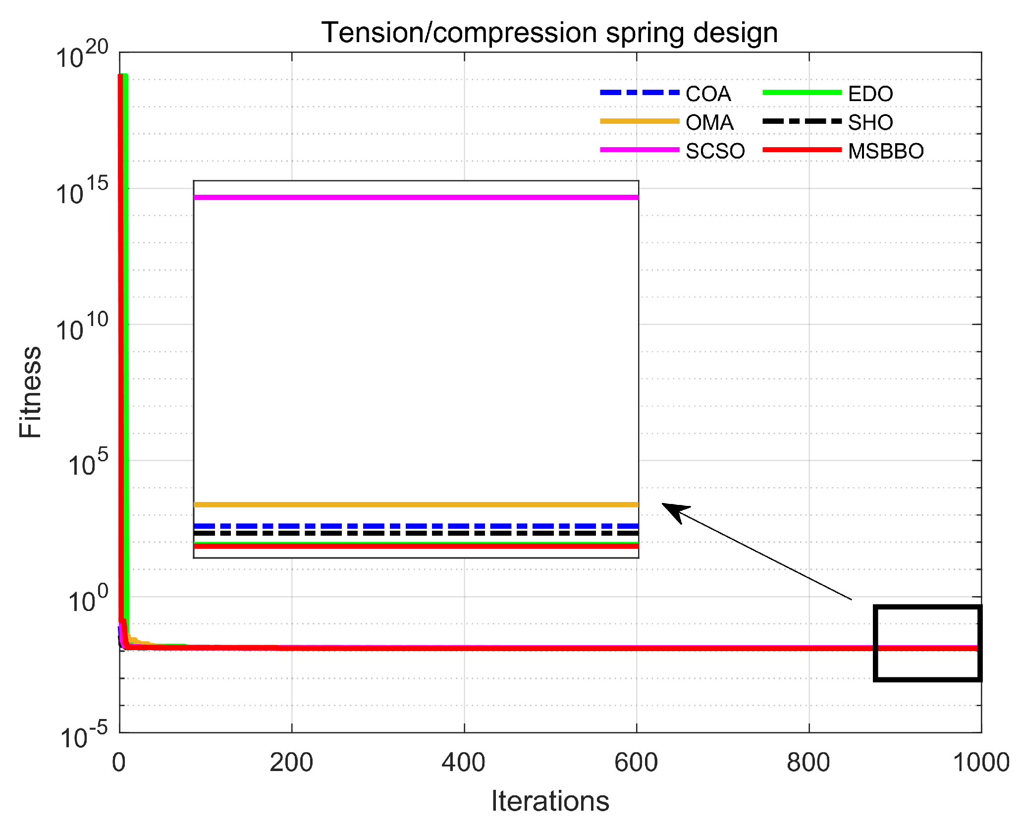
The tension/compression spring design problem is to minimize the weight of the spring while meeting the constraints of minimum deflection, vibration frequency, and shear stress [69]. As shown in Figure 12, it consists of three variables: the wire diameter (d), the mean coil diameter (D) and the number of active coils (P). The mathematical model is given in Equation (15). The results are summarized in Table 8, and the convergence curves are shown in Figure 13. It is not difficult to find that MSBBO finds the value of the objective function (0.01266959) with higher precision when all variables conform to the constraint. In contrast, the results of COA, EDO and SHO are also very close to our algorithm. As new optimization techniques, they also provide reliable solutions.
X = x 1 , x 2 , x 3 = [ d , D , P ] minimize f ( X ) = x 3 + 2 x 2 x 1 2 s . t . g 1 ( X ) = 1 x 2 3 x 3 71785 x 1 4 0 g 2 ( X ) = 4 x 2 2 x 1 x 2 12566 x 2 x 1 3 x 1 4 + 1 5108 x 1 2 1 0 g 3 ( X ) = 1 140.45 x 1 x 2 2 x 3 0 g 4 ( X ) = x 1 + x 2 1.5 1 0 where 0.05 x 1 2 , 0.25 x 2 1.3 , 2 x 3 15 .

5.6.3. Welded Beam Design

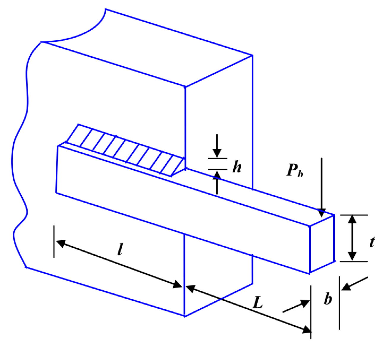
The objective of the welding beam design problem is to obtain the minimum manufacturing cost [70]. As shown in Figure 14, this optimization problem has four variables that need to be calculated: the thickness of the weld (h), the length of the attached part of the bar (l), the height of the bar (t), and the thickness of the bar (b). Then, there are seven constraints that need to be satisfied in this optimization design [70]. These constraints include shear stress ( τ ), bending stress in beam ( σ ), deflection of beam end ( δ ) and buckling load of bar ( P b ). The mathematical model of this problem is given in Equation (16). Similarly, Table 9 shows the optimal results of the six comparison algorithms, and Figure 15 shows the convergence curves of the objective function on the welded beam design problem.
x = x 1 x 2 x 3 x 4 = [ h , l , t , b ] minimize f ( x ) = 1.10471 x 1 2 x 2 + 0.04811 x 3 x 4 14.0 + x 2 , g 1 ( x ) = τ ( x ) τ max 0 , g 2 ( x ) = σ ( x ) σ max 0 , g 3 ( x ) = δ ( x ) δ max 0 , g 4 ( x ) = x 1 x 4 0 , g 5 ( x ) = P P c ( x ) 0 , g 6 ( x ) = 0.125 x 1 0 , g 7 ( x ) = 1.10471 x 1 2 x 2 + 0.04811 x 3 x 4 14.0 + x 2 5.0 0 0.1 x 1 2 , 0.1 x 2 10 , 0.1 x 3 10 0.1 x 4 2 τ ( x ) = τ 2 + 2 τ τ x 2 2 R + τ 2 , τ = p 2 x 1 x 2 , τ = M R J , M = P L + x 2 2 , R = x 2 2 4 + x 1 + x 3 2 2 , J = 2 2 x 1 x 2 x 2 2 4 + x 1 + x 3 2 2 , σ ( x ) = 6 P L x 4 x 3 2 , δ ( x ) = 6 P L 3 E x 3 2 x 4 P c ( x ) = 4.013 E x 3 2 x 4 6 36 L 2 1 x 3 2 L E 4 G , P = 6000   lb ,   L = 14   in . , δ max = 0.25   in . , E = 30 × 10 6   psi ,   G = 12 × 10 6   psi , τ max = 13,600   psi ,   σ max = 30,000   psi
According to the experimental results, MSBBO and OMA search for the same optimal solution: [h, l, t, b] = [0.19883231, 3.33736530, 9.19202432, 0.19883231]. The values of the variables obtained by the two algorithms are exactly equal (1.67021773). This shows that the performance of the two methods is not significantly different on the welded beam design problem. As a newly proposed optimization technique, OMA has been fully tested theoretically. Therefore, it can be considered that the solving ability of MSBBO on this problem has reached the level of advanced optimization technology.

5.6.4. Speed Reducer Design

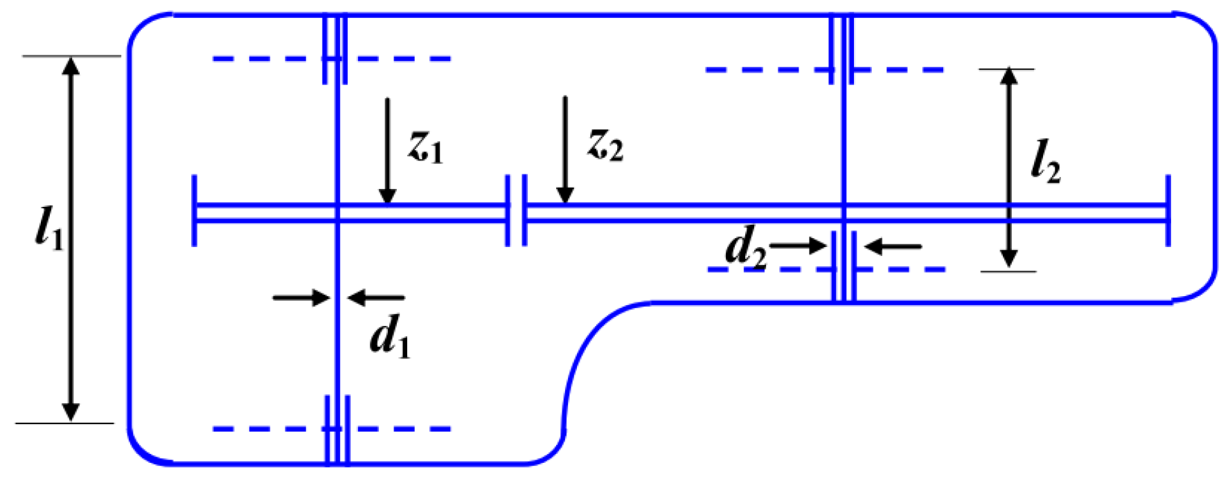
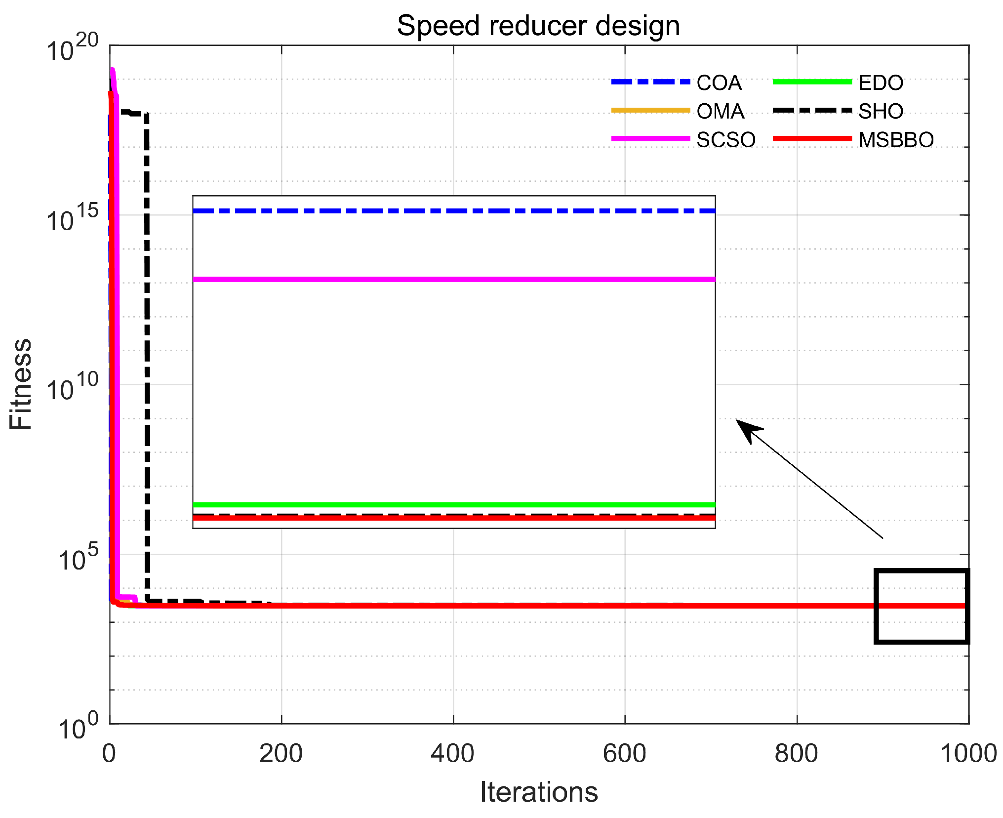
The purpose of the speed reducer design problem is to minimize the cost when the 11 constraints are met [71]. The problem consists of seven decision variables as shown in Figure 16. Its mathematical model is shown in Equation (17). Similarly, six optimization methods are used to search for optimal decision variables and objective function values for this problem. The experimental results and convergence curves are shown in Table 10 and Figure 17, respectively. It can be found that MSBBO also obtains the optimal objective function value of the six algorithms. In addition, the EDO, OMA and SHO calculations are also very close to our work, and the solutions they provide are also worth referring to.
x = x 1 , x 2 , x 3 , x 4 , x 5 , x 6 , x 7 = b , m , z , l 1 , l 2 , d 1 , d 2 minimize f 4 ( x ) = 0.7854 x 1 x 2 2 3.3333 x 3 2 + 14.9334 x 3 43.0934 1.508 x 1 x 6 2 + x 7 2 + 0.7854 x 1 x 4 x 6 2 x 5 x 7 2 . g 1 ( x ) = 27 x 1 x 2 2 x 3 1 0 , g 2 ( x ) = 397.5 x 1 x 2 2 x 3 2 1 0 , g 3 ( x ) = 1.93 x 4 2 x 2 x 6 4 x 3 1 0 , g 4 ( x ) = 1.93 x 5 2 x 2 x 7 4 x 3 1 0 , g 5 ( x ) = 74 x 4 x 2 x 3 2 + 16.9 × 10 6 0.5 110 x 6 3 1 0 , g 6 ( x ) = 745 x 5 x 2 x 3 2 + 157.5 × 10 6 0.5 85 x 7 3 1 0 , g 7 ( x ) = x 2 x 3 40 1 0 , g 8 ( x ) = 5 x 2 x 1 1 0 , g 9 ( x ) = x 1 12 x 2 1 0 , g 10 ( x ) = 1.5 x 6 + 1.9 x 4 1 0 , g 11 ( x ) = 1.1 x 7 + 1.9 x 5 1 0 . where 2.6 x 1 3.6 , 0.7 x 2 0.8 , 17 x 3 28 , 7.3 x 4 8.3 , 7.3 x 5 8.3 , 2.9 x 6 3.9 , 5.0 x 7 5.5 .

5.6.5. Step-Cone Pulley Problem

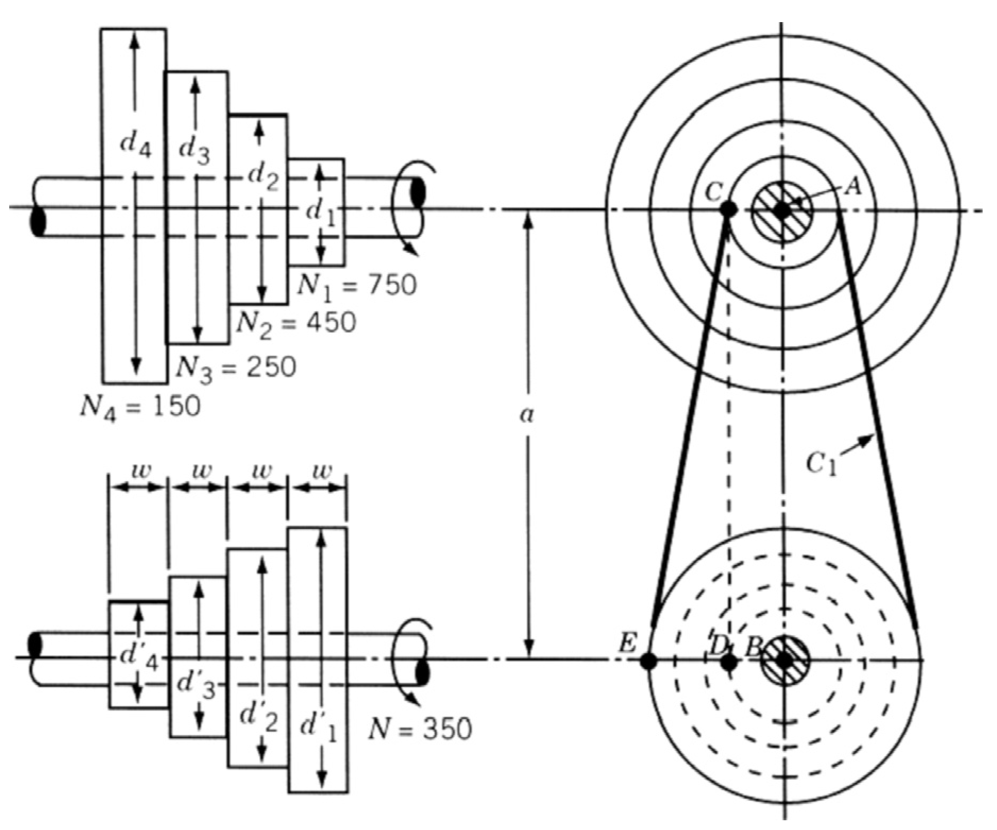
This problem requires the design of a step-cone pulley based on the values of five decision variables [72]. Among them, the four design variables are the diameter of each step ( d 1 , d 2 , d 3 , d 4 ), and the last design variable is the width of the pulley (w) as shown in Figure 18. The problem consists of 11 constraint adjustments, of which 3 are equality constraints and 8 are inequality constraints, to ensure that all step sizes, tension ratios, and belt transfer power are the same. Its mathematical model is shown in Equation (18).
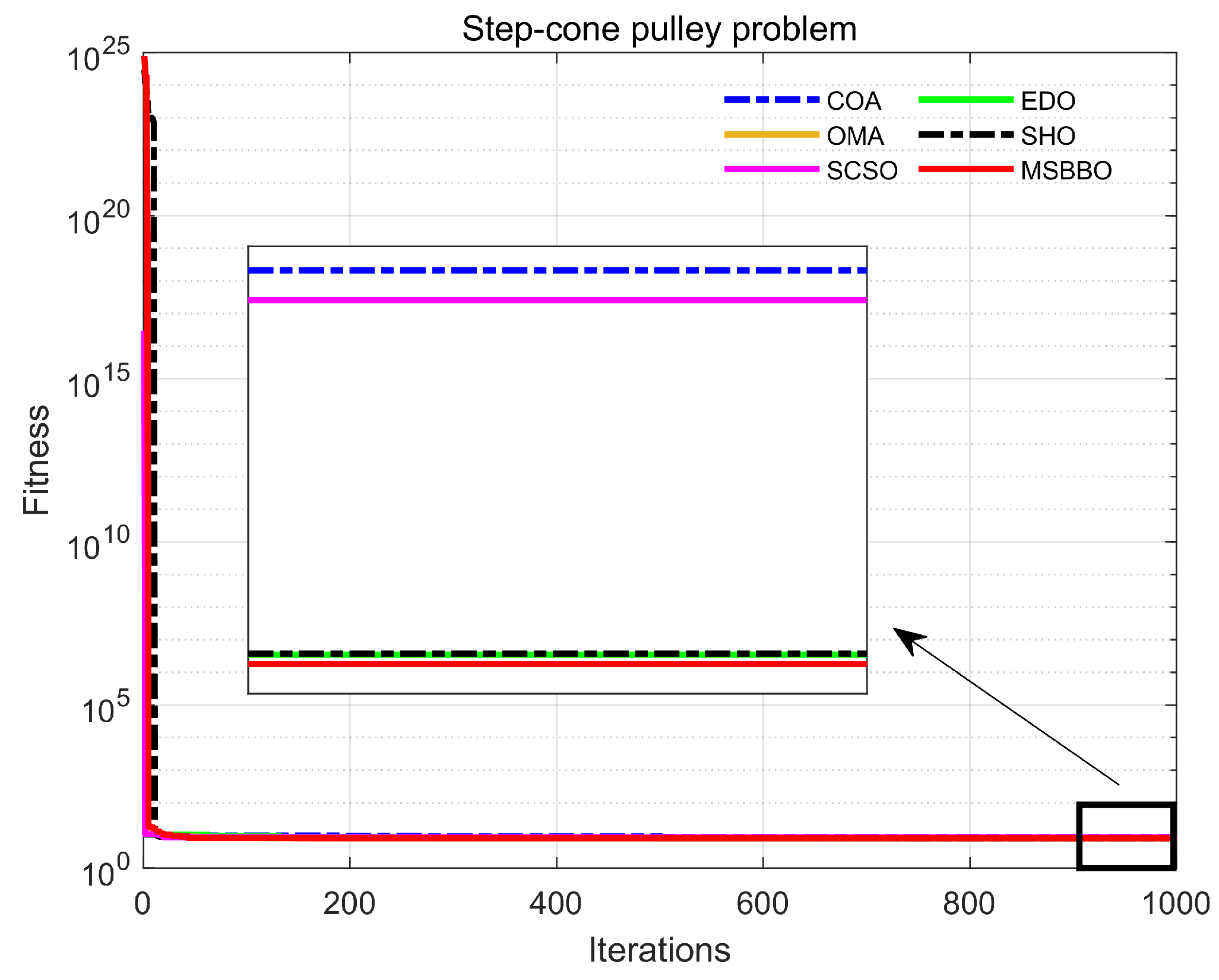
For the sake of discussion, Table 11 shows the optimal results of all comparison algorithms, and Figure 19 shows their convergence curves on this problem. According to the results in Table 11, it can be concluded that MSBBO can still obtain the ideal optimal solution in several advanced algorithms on the step-cone pulley problem. In addition, OMA also obtains the same precision as the MSBBO objective function value (8.18149598). In Figure 19, the MSBBO convergence curve is at the bottom and coincides with the OMA convergence curve. But they have different decision variable values. This shows that the optimal solution of the same problem is not unique, and our work provides new design parameter values for the step-cone pulley problem: [ d 1 , d 2 , d 3 , d 4 , w] = [16.96572695, 28.25753037, 50.79673307, 84.49572374, 89.99999337].
minimize : f ( x ¯ ) = ρ ω d 1 2 11 + N 1 N 2 + d 2 2 1 + N 2 N 2 + d 3 2 1 + N 3 N 2 + d 4 2 1 + N 4 N 2 h 1 ( x ¯ ) = C 1 C 2 = 0 , h 2 ( x ¯ ) = C 1 C 3 = 0 , h 3 ( x ¯ ) = C 1 C 4 = 0 g i = 1 , 2 , 3.4 ( x ¯ ) = R i 2 , g i = 1 , 2 , 3.4 ( x ¯ ) = ( 0.75 × 745.6998 ) P i 0 C i = π d i 2 1 + N i N + N i N 1 2 4 a + 2 a , i = ( 1 , 2 , 3 , 4 ) R i = exp μ π 2 sin 1 N i N 1 d i 2 a , i = ( 1 , 2 , 3 , 4 ) P i = st ! 1 R i π d i N i 60 , i = ( 1 , 2 , 3 , 4 ) , t = 8 mm s = 1.75 MPa , μ = 0.35 , ρ = 7200 kg / m 3 , a = 3 mm

5.6.6. Robot Gripper Problem

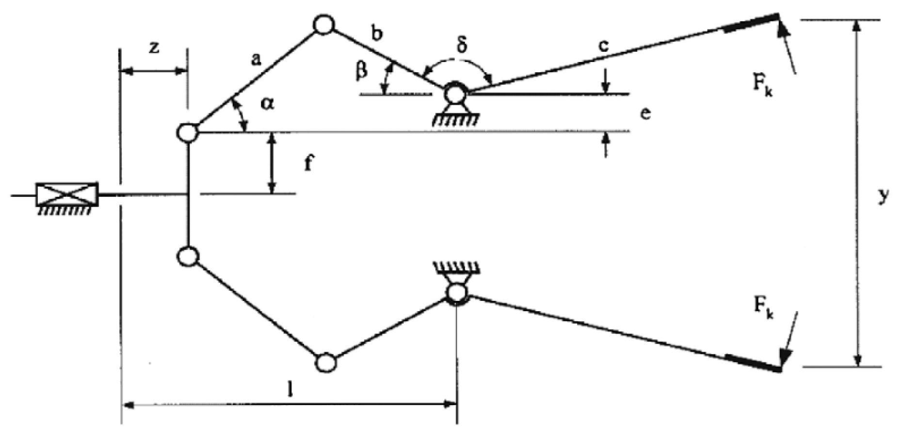
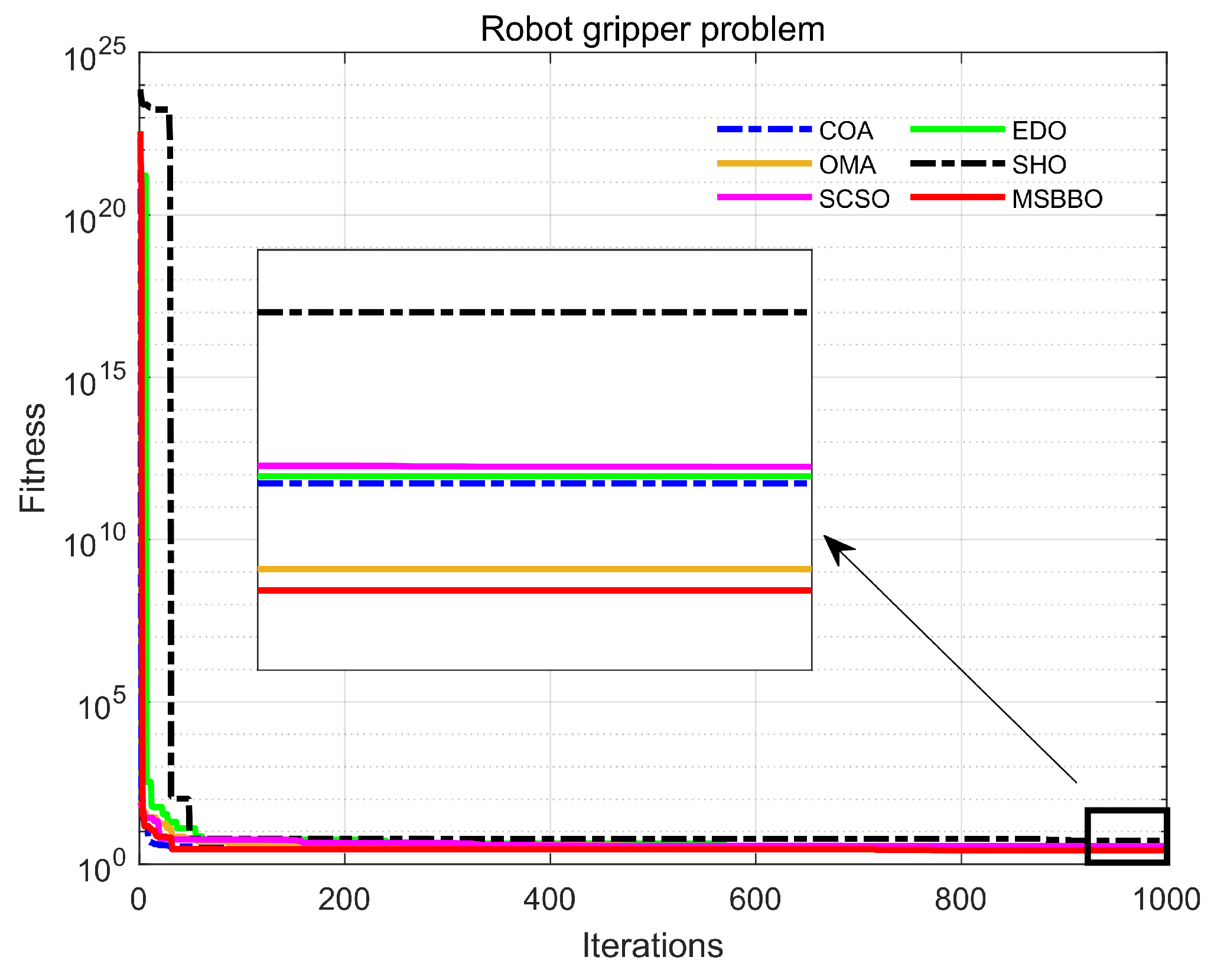
The optimization goal of the robot gripper problem is to minimize the difference between the maximum and minimum force [73]. It is by the gripper end displacement of the range applied to the gripper. This problem consists of seven consecutive decision variables: a , b , c , d , e , f and δ as shown in Figure 20. The robot gripper problem needs to satisfy seven inequality constraints, which is complex. Its mathematical model is shown in Equation (19). As with the other problems, the results of the six comparison algorithms are summarized in Table 12, and Figure 21 shows their convergence curves. It is not difficult to see that MSBBO, as an enhanced variant of BBO, is significantly better than the other five new meta-heuristic algorithms when seven inequality constraints are met. This shows that our improvement strategies have effectively enhanced the application value of BBO. Therefore, MSBBO can also be widely used on engineering constrained optimization problems.
minimize f ( x ) = max z F k ( x , z ) min z F k ( x , z ) g 1 ( x ) = Y min y x , Z max 0 , g 2 ( x ) = y x , Z max 0 , g 3 ( x ) = y ( x , 0 ) Y max 0 , g 4 ( x ) = Y G y ( x , 0 ) 0 , g 5 ( x ) = ( a + b ) 2 l 2 e 2 0 , g 6 ( x ) = l Z max 2 + ( a e ) 2 b 2 0 , g 7 ( x ) = l Z max 0 , g = ( l z ) 2 + e 2 , α = arccos a 2 + g 2 b 2 2 a g + ϕ β = arccos b 2 + g 2 a 2 2 b g ϕ ϕ = arctan e l z + ϕ , F k = P b sin ( α + β ) 2 c cos ( α ) y ( x , z ) = 2 ( e + f + c sin ( β + δ ) ) Y min = 50 , Y max = 100 , P = 100 Y G = 150 , Z max = 100 , P 0 c 200 10 a , b , f 150 , 100 c 1 δ 3.14 0 e 50 , 100 l 300 , 1 δ

6. Conclusions

This paper proposes a comprehensive multi-strategy enhanced BBO variant. Firstly, the example chasing strategy is proposed to effectively maintain the population diversity. Then, the heuristic crossover strategy is designed to enhance the search ability of the algorithm. Finally, the prey search–attack strategy is designed to balance the exploration and exploitation of the algorithm, which improves the convergence accuracy and speed effectively. MSBBO makes BBO suitable for high-dimensional optimization environments. Compared to other BBO variants (PRBBO, BBOSB, HGBBO, FABBO, BLEHO, MPBBO and BBOIMAM), MSBBO uses only three improvement strategies to greatly improve the BBO convergence performance, which enables it to effectively solve high-dimensional optimization problems and has simpler computational complexity than the original BBO. At the same time, MSBBO is compared with seven latest meta-heuristic algorithms (GWO, WOA, SSA, ChOA, MPA, GJO and BWO). Experimental results show that MSBBO has better performance than all compared algorithms and is more suitable for solving large-scale optimization problems. Further, MSBBO and five new optimization techniques (COA, EDO, OMA, SHO and SCSO) are used to solve six engineering problems, and the results show that our work is also more competitive than these new optimization techniques.
Because the algorithm can effectively balance exploration and exploitation, and can adapt to high-dimensional optimization environments, it is expected to perform well in multi-objective problems. In addition, in the case of hardware equipment, we can try to implement this algorithm in a distributed way and solve more complex practical problems. Therefore, we plan to implement it in a distributed manner in future studies. Moreover, it can also be combined with other techniques in the search area of optimization problems, such as local or global search methods, to improve its performance. Meanwhile, it can be used to solve many complex problems, such as feature selection, image segmentation, job-shop scheduling and vehicle routing problems, as well as optimization node positioning problems in systems. Therefore, we will pay more attention to the application of the MSBBO algorithm for complex optimization problems in the future.

Author Contributions

C.G.: Investigation, Methodology, Experiment, Writing—original draft. T.L.: Supervision, Funding acquisition. Y.G.: Funding acquisition, Writing—review and editing. Z.Z.: Data curation, Writing—review and editing. All authors have read and agreed to the published version of the manuscript.

Funding

This work was supported by the Key Project of Ningxia Natural Science Foundation [2022AAC02043]. the National Natural Science Foundation of China under Grant [61902291], the Construction Project of First-class Subjects in Ningxia Higher Education [NXYLXK2017B09], and the Major Proprietary Funded Project of North Minzu University [ZDZX201901].

Data Availability Statement

All the data in Section 5 were obtained under the same experimental environment. Then, all the source programs of the compared BBO variants in Section 5.3 are coded according to their original references. We solemnly declare that all data in this paper are true and valid.

Conflicts of Interest

The authors declare that they have no known competing financial interests or personal relationships that could have appeared to influence the work reported in this paper. All authors guarantee that the paper is legitimate and belongs to their own scientific research results.

References

  1. Qian, K.; Liu, Y.; Tian, L.; Bao, J. Robot path planning optimization method based on heuristic multi-directional rapidly-exploring tree. Comput. Electr. Eng. 2020, 85, 106688. [Google Scholar] [CrossRef]
  2. Islam, M.A.; Gajpal, Y.; ElMekkawy, T.Y. Hybrid particle swarm optimization algorithm for solving the clustered vehicle routing problem. Appl. Soft Comput. 2021, 110, 107655. [Google Scholar] [CrossRef]
  3. Ertenlice, O.; Kalayci, C.B. A survey of swarm intelligence for portfolio optimization: Algorithms and applications. Swarm Evol. Comput. 2018, 39, 36–52. [Google Scholar] [CrossRef]
  4. Ding, H.; Gu, X. Hybrid of human learning optimization algorithm and particle swarm optimization algorithm with scheduling strategies for the flexible job-shop scheduling problem. Neurocomputing 2020, 414, 313–332. [Google Scholar] [CrossRef]
  5. Darvish, A.; Ebrahimzadeh, A. Improved fruit-fly optimization algorithm and its applications in antenna arrays synthesis. IEEE Trans. Antennas Propag. 2018, 66, 1756–1766. [Google Scholar] [CrossRef]
  6. Liu, Y.; Jin, S.; Zhou, J.; Hu, Q. A branch-and-bound algorithm for the unit-capacity resource constrained project scheduling problem with transfer times. Comput. Oper. Res. 2023, 151, 106097. [Google Scholar] [CrossRef]
  7. Babaie-Kafaki, S. A survey on the Dai–Liao family of nonlinear conjugate gradient methods. Rairo-Oper. Res. 2023, 57, 43–58. [Google Scholar] [CrossRef]
  8. Mittal, G.; Giri, A.K. A modified steepest descent method for solving non-smooth inverse problems. J. Comput. Appl. Math. 2023, 424, 114997. [Google Scholar] [CrossRef]
  9. Holland, J. Adaptation in Natural and Artificial Systems: An Introductory Analysis with Application to Biology, Control and Artificial Intelligence; University of Michigan Press: Ann Arbor, MI, USA, 1975. [Google Scholar]
  10. Storn, R.; Price, K. Differential evolution—A simple and efficient heuristic for global optimization over continuous spaces. J. Glob. Optim. 1997, 11, 341. [Google Scholar] [CrossRef]
  11. Dasgupta, D. An artificial immune system as a multi-agent decision support system. In Proceedings of the SMC’98 Conference Proceedings. 1998 IEEE International Conference on Systems, Man, and Cybernetics (Cat. No. 98CH36218), San Diego, CA, USA, 14 October 1998; Volume 4, pp. 3816–3820. [Google Scholar] [CrossRef]
  12. Kennedy, J.; Eberhart, R. Particle swarm optimization. In Proceedings of the ICNN’95 International Conference on Neural Networks, Perth, WA, Australia, 27 November–1 December 1995; Volume 4, pp. 1942–1948. [Google Scholar] [CrossRef]
  13. Mirjalili, S.; Lewis, A. The whale optimization algorithm. Adv. Eng. 2016, 95, 51–67. [Google Scholar] [CrossRef]
  14. Xue, J.; Shen, B. A novel swarm intelligence optimization approach: Sparrow search algorithm. Syst. Sci. Control. Eng. 2020, 8, 22–34. [Google Scholar] [CrossRef]
  15. Simon, D. Biogeography-based optimization. IEEE Trans. Evol. Comput. 2008, 12, 702–713. [Google Scholar] [CrossRef]
  16. Xing, B.; Gao, W.J.; Xing, B.; Gao, W.J. Invasive weed optimization algorithm. In Innovative Computational Intelligence: A Rough Guide to 134 Clever Algorithms; Springer: Cham, Switzerland, 2014; pp. 177–181. [Google Scholar] [CrossRef]
  17. Kiran, M.S. TSA: Tree-seed algorithm for continuous optimization. Expert Syst. Appl. 2015, 42, 6686–6698. [Google Scholar] [CrossRef]
  18. Hashim, F.A.; Hussain, K.; Houssein, E.H.; Mabrouk, M.S.; Al-Atabany, W. Archimedes optimization algorithm: A new metaheuristic algorithm for solving optimization problems. Appl. Intell. 2021, 51, 1531–1551. [Google Scholar] [CrossRef]
  19. Abdel-Basset, M.; Mohamed, R.; Azeem, S.A.A.; Jameel, M.; Abouhawwash, M. Kepler optimization algorithm: A new metaheuristic algorithm inspired by Kepler’s laws of planetary motion. Knowl.-Based Syst. 2023, 268, 110454. [Google Scholar] [CrossRef]
  20. Abdel-Basset, M.; El-Shahat, D.; Jameel, M.; Abouhawwash, M. Young’s double-slit experiment optimizer: A novel metaheuristic optimization algorithm for global and constraint optimization problems. Comput. Methods Appl. Mech. Eng. 2023, 403, 115652. [Google Scholar] [CrossRef]
  21. Das, B.; Mukherjee, V.; Das, D. Student psychology based optimization algorithm: A new population based optimization algorithm for solving optimization problems. Adv. Eng. Softw. 2020, 146, 102804. [Google Scholar] [CrossRef]
  22. Rao, R.V.; Savsani, V.J.; Vakharia, D.P. Teaching–learning-based optimization: An optimization method for continuous non-linear large scale problems. Inf. Sci. 2012, 183, 1–15. [Google Scholar] [CrossRef]
  23. Ahmadi, S.A. Human behavior-based optimization: A novel metaheuristic approach to solve complex optimization problems. Neural Comput. Appl. 2017, 28 (Suppl. S1), 233–244. [Google Scholar] [CrossRef]
  24. Chakraborty, S.; Saha, A.K.; Chakraborty, R.; Saha, M. An enhanced whale optimization algorithm for large scale optimization problems. Knowl.-Based Syst. 2021, 233, 107543. [Google Scholar] [CrossRef]
  25. Rivera, M.M.; Guerrero-Mendez, C.; Lopez-Betancur, D.; Saucedo-Anaya, T. Dynamical Sphere Regrouping Particle Swarm Optimization: A Proposed Algorithm for Dealing with PSO Premature Convergence in Large-Scale Global Optimization. Mathematics 2023, 11, 4339. [Google Scholar] [CrossRef]
  26. Long, W.; Wu, T.; Liang, X.; Xu, S. Solving high-dimensional global optimization problems using an improved sine cosine algorithm. Expert Syst. Appl. 2019, 123, 108–126. [Google Scholar] [CrossRef]
  27. Goel, L. A novel approach for face recognition using biogeography based optimization with extinction and evolution. Multimed. Tools Appl. 2022, 81, 10561–10588. [Google Scholar] [CrossRef]
  28. Jain, A.; Rai, S.; Srinivas, R.; Al-Raoush, R.I. Bioinspired modeling and biogeography-based optimization of electrocoagulation parameters for enhanced heavy metal removal. J. Clean. Prod. 2022, 338, 130622. [Google Scholar] [CrossRef]
  29. Zhang, Z.; Gao, Y.; Zuo, W. A dual biogeography-based optimization algorithm for solving high-dimensional global optimization problems and engineering design problems. IEEE Access 2022, 10, 55988–56016. [Google Scholar] [CrossRef]
  30. Zhang, Q.; Wei, L.; Yang, B. Research on Improved BBO Algorithm and Its Application in Optimal Scheduling of Micro-Grid. Mathematics 2022, 10, 2998. [Google Scholar] [CrossRef]
  31. Ma, H.; Simon, D.; Siarry, P.; Yang, Z.; Fei, M. Biogeography-based optimization: A 10-year review. IEEE Trans. Emerg. Top. Comput. Intell. 2017, 1, 391–407. [Google Scholar] [CrossRef]
  32. Ergezer, M.; Simon, D.; Du, D. Oppositional biogeography-based optimization. In Proceedings of the 2009 IEEE International Conference on Systems, Man and Cybernetics, San Antonio, TX, USA, 11–14 October 2009; pp. 1009–1014. [Google Scholar] [CrossRef]
  33. Wang, G.G.; Gandomi, A.H.; Alavi, A.H. An effective krill herd algorithm with migration operator in biogeography-based optimization. Appl. Math. Model. 2014, 38, 2454–2462. [Google Scholar] [CrossRef]
  34. Lohokare, M.R.; Panigrahi, B.K.; Pattnaik, S.S.; Devi, S.; Mohapatra, A. Neighborhood search-driven accelerated biogeography-based optimization for optimal load dispatch. IEEE Trans. Syst. Man Cybern. Part Appl. Rev. 2012, 42, 641–652. [Google Scholar] [CrossRef]
  35. Chen, X.; Tianfield, H.; Du, W.; Liu, G. Biogeography-based optimization with covariance matrix based migration. Appl. Soft Comput. 2016, 45, 71–85. [Google Scholar] [CrossRef]
  36. Sang, X.; Liu, X.; Zhang, Z.; Wang, L. Improved biogeography-based optimization algorithm by hierarchical tissue-like P system with triggering ablation rules. Math. Probl. Eng. 2021, 2021, 6655614. [Google Scholar] [CrossRef]
  37. Zhang, Z.; Gao, Y.; Liu, Y.; Zuo, W. A hybrid biogeography-based optimization algorithm to solve high-dimensional optimization problems and real-world engineering problems. Appl. Soft Comput. 2023, 144, 110514. [Google Scholar] [CrossRef]
  38. Zhang, Z.; Gao, Y.; Guo, E. A supercomputing method for large-scale optimization: A feedback biogeography-based optimization with steepest descent method. J. Supercomput. 2023, 79, 1318–1373. [Google Scholar] [CrossRef]
  39. Garg, V.; Deep, K. Performance of Laplacian Biogeography-Based Optimization Algorithm on CEC 2014 continuous optimization benchmarks and camera calibration problem. Swarm Evol. Comput. 2016, 27, 132–144. [Google Scholar] [CrossRef]
  40. Zhao, F.; Qin, S.; Zhang, Y.; Ma, W.; Zhang, C.; Song, H. A two-stage differential biogeography-based optimization algorithm and its performance analysis. Expert Syst. Appl. 2019, 115, 329–345. [Google Scholar] [CrossRef]
  41. Khademi, G.; Mohammadi, H.; Simon, D. Hybrid invasive weed/biogeography-based optimization. Eng. Appl. Artif. Intell. 2017, 64, 213–231. [Google Scholar] [CrossRef]
  42. Zhang, X.; Wang, D.; Fu, Z.; Liu, S.; Mao, W.; Liu, G.; Jiang, Y.; Li, S. Novel biogeography-based optimization algorithm with hybrid migration and global-best Gaussian mutation. Appl. Math. Model. 2020, 86, 74–91. [Google Scholar] [CrossRef]
  43. Zhang, X.; Kang, Q.; Tu, Q.; Cheng, J.; Wang, X. Efficient and merged biogeography-based optimization algorithm for global optimization problems. Soft Comput. 2019, 23, 4483–4502. [Google Scholar] [CrossRef]
  44. Reihanian, A.; Feizi-Derakhshi, M.R.; Aghdasi, H.S. NBBO: A new variant of biogeography-based optimization with a novel framework and a two-phase migration operator. Inf. Sci. 2019, 504, 178–201. [Google Scholar] [CrossRef]
  45. Gerton, J.L.; Hawley, R.S. Homologous chromosome interactions in meiosis: Diversity amidst conservation. Nat. Rev. Genet. 2005, 6, 477–487. [Google Scholar] [CrossRef]
  46. Dhiman, G.; Garg, M.; Nagar, A.; Kumar, V.; Dehghani, M. A novel algorithm for global optimization: Rat swarm optimizer. J. Ambient. Intell. Humaniz. Comput. 2021, 12, 8457–8482. [Google Scholar] [CrossRef]
  47. Derrac, J.; García, S.; Molina, D.; Herrera, F. A practical tutorial on the use of nonparametric statistical tests as a methodology for comparing evolutionary and swarm intelligence algorithms. Swarm Evol. Comput. 2011, 1, 3–18. [Google Scholar] [CrossRef]
  48. Atanassov, K.; Vassilev, P. Intuitionistic fuzzy sets and other fuzzy sets extensions representable by them. J. Intell. Fuzzy Syst. 2020, 38, 525–530. [Google Scholar] [CrossRef]
  49. Atanassov, K. Intuitionistic fuzzy modal topological structure. Mathematics 2022, 10, 3313. [Google Scholar] [CrossRef]
  50. Feng, Q.; Liu, S.; Zhang, J.; Yang, G.; Yong, L. Improved biogeography-based optimization with random ring topology and Powell’s method. Appl. Math. Model. 2017, 41, 630–649. [Google Scholar] [CrossRef]
  51. Xiong, G.; Shi, D. Hybrid biogeography-based optimization with brain storm optimization for non-convex dynamic economic dispatch with valve-point effects. Energy 2018, 157, 424–435. [Google Scholar] [CrossRef]
  52. Farrokh Ghatte, H. A hybrid of firefly and biogeography-based optimization algorithms for optimal design of steel frames. Arab. J. Sci. Eng. 2021, 46, 4703–4717. [Google Scholar] [CrossRef]
  53. Li, W.; Wang, G.G. Elephant herding optimization using dynamic topology and biogeography-based optimization based on learning for numerical optimization. Eng. Comput. 2022, 38 (Suppl. S2), 1585–1613. [Google Scholar] [CrossRef]
  54. Zhang, X.; Wen, S.; Wang, D. Multi-population biogeography-based optimization algorithm and its application to image segmentation. Appl. Soft Comput. 2022, 124, 109005. [Google Scholar] [CrossRef]
  55. Liang, S.; Fang, Z.; Sun, G.; Qu, G. Biogeography-based optimization with adaptive migration and adaptive mutation with its application in sidelobe reduction of antenna arrays. Appl. Soft Comput. 2022, 121, 108772. [Google Scholar] [CrossRef]
  56. Mirjalili, S.; Mirjalili, S.M.; Lewis, A. Grey wolf optimizer. Adv. Eng. Softw. 2014, 69, 46–61. [Google Scholar] [CrossRef]
  57. Jain, M.; Singh, V.; Rani, A. A novel nature-inspired algorithm for optimization: Squirrel search algorithm. SWarm Evol. Comput. 2019, 44, 148–175. [Google Scholar] [CrossRef]
  58. Khishe, M.; Mosavi, M.R. Chimp optimization algorithm. Expert Syst. Appl. 2020, 149, 113338. [Google Scholar] [CrossRef]
  59. Faramarzi, A.; Heidarinejad, M.; Mirjalili, S.; Gandomi, A.H. Marine Predators Algorithm: A nature-inspired metaheuristic. Expert Syst. Appl. 2020, 152, 113377. [Google Scholar] [CrossRef]
  60. Chopra, N.; Ansari, M.M. Golden jackal optimization: A novel nature-inspired optimizer for engineering applications. Expert Syst. Appl. 2022, 198, 116924. [Google Scholar] [CrossRef]
  61. Zhong, C.; Li, G.; Meng, Z. Beluga whale optimization: A novel nature-inspired metaheuristic algorithm. Knowl.-Based Syst. 2022, 251, 109215. [Google Scholar] [CrossRef]
  62. Dehghani, M.; Montazeri, Z.; Trojovská, E.; Trojovský, P. Coati Optimization Algorithm: A new bio-inspired metaheuristic algorithm for solving optimization problems. Knowl.-Based Syst. 2023, 259, 110011. [Google Scholar] [CrossRef]
  63. Abdel-Basset, M.; El-Shahat, D.; Jameel, M.; Abouhawwash, M. Exponential distribution optimizer (EDO): A novel math-inspired algorithm for global optimization and engineering problems. Artif. Intell. Rev. 2023, 56, 9329–9400. [Google Scholar] [CrossRef]
  64. Cheng, M.Y.; Sholeh, M.N. Optical microscope algorithm: A new metaheuristic inspired by microscope magnification for solving engineering optimization problems. Knowl.-Based Syst. 2023, 279, 110939. [Google Scholar] [CrossRef]
  65. Zhao, S.; Zhang, T.; Ma, S.; Wang, M. Sea-horse optimizer: A novel nature-inspired meta-heuristic for global optimization problems. Appl. Intell. 2023, 53, 11833–11860. [Google Scholar] [CrossRef]
  66. Seyyedabbasi, A.; Kiani, F. Sand Cat swarm optimization: A nature-inspired algorithm to solve global optimization problems. Eng. Comput. 2023, 39, 2627–2651. [Google Scholar] [CrossRef]
  67. Wang, L.; Cao, Q.; Zhang, Z.; Mirjalili, S.; Zhao, W. Artificial rabbits optimization: A new bio-inspired meta-heuristic algorithm for solving engineering optimization problems. Eng. Appl. Artif. Intell. 2022, 114, 105082. [Google Scholar] [CrossRef]
  68. Trojovská, E.; Dehghani, M.; Trojovský, P. Zebra optimization algorithm: A new bio-inspired optimization algorithm for solving optimization algorithm. IEEE Access 2022, 10, 49445–49473. [Google Scholar] [CrossRef]
  69. Hashim, F.A.; Houssein, E.H.; Hussain, K.; Mabrouk, M.S.; Al-Atabany, W. Honey Badger Algorithm: New metaheuristic algorithm for solving optimization problems. Math. Comput. Simul. 2022, 192, 84–110. [Google Scholar] [CrossRef]
  70. Yapici, H.; Cetinkaya, N. A new meta-heuristic optimizer: Pathfinder algorithm. Appl. Soft Comput. 2019, 78, 545–568. [Google Scholar] [CrossRef]
  71. Zhao, W.; Zhang, Z.; Wang, L. Manta ray foraging optimization: An effective bio-inspired optimizer for engineering applications. Eng. Appl. Artif. Intell. 2020, 87, 103300. [Google Scholar] [CrossRef]
  72. Savsani, P.; Savsani, V. Passing vehicle search (PVS): A novel metaheuristic algorithm. Appl. Math. Model. 2016, 40, 3951–3978. [Google Scholar] [CrossRef]
  73. Krenich, S.; Osyczka, A. Optimization of Robot Gripper Parameters Using Genetic Algorithms. In Romansy 13; Springer: Vienna, Austria, 2000. [Google Scholar] [CrossRef]
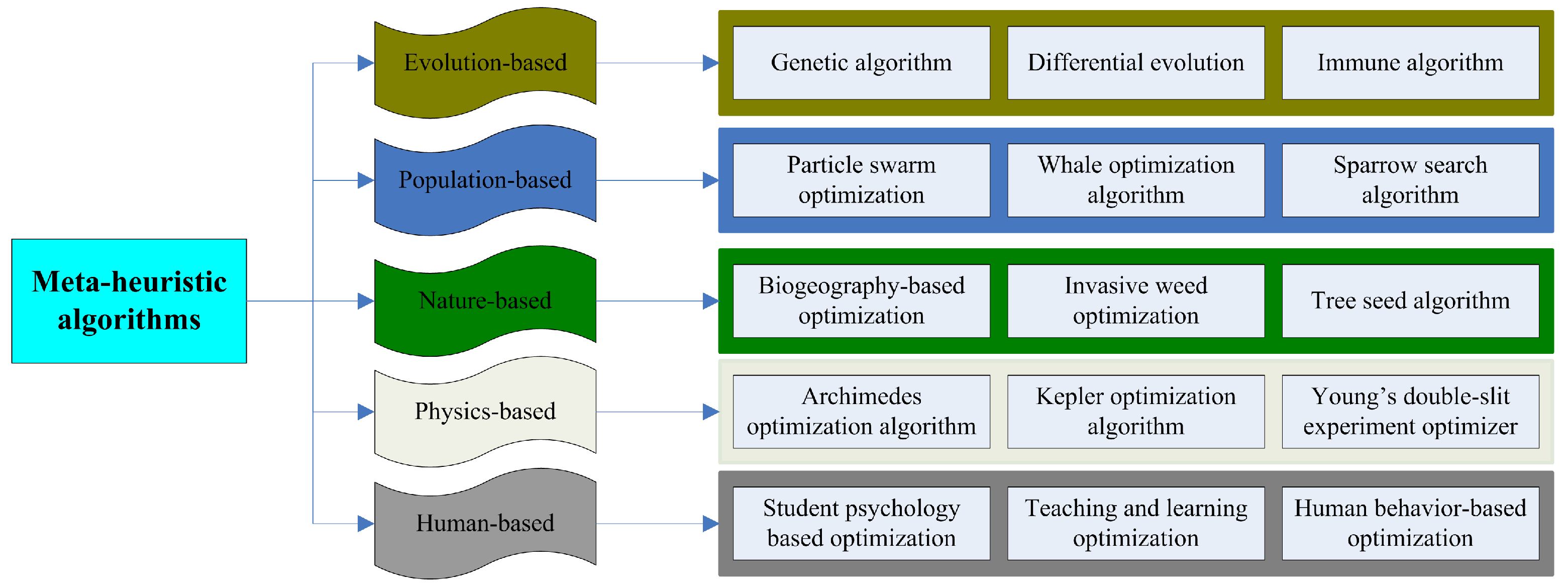
Figure 1. Meta-heuristic algorithm classification.
Mathematics 12 00435 g001
Figure 2. BBO articles’ source statistics.
Mathematics 12 00435 g002
Figure 3. Graphical abstract of this paper.
Mathematics 12 00435 g003
Figure 4. Random migration vs. the example chasing strategy.
Mathematics 12 00435 g004
Figure 5. Convergence curves and boxplots of MSBBO and BBO on different benchmark functions ( D = 30 , 50 , 100 ).
Mathematics 12 00435 g005
Figure 6. Average running seconds of BBO and MSBBO on each function ( D = 100 ).
Mathematics 12 00435 g006
Figure 7. Convergence curves and boxplots of MSBBO and BBO variants on different benchmark functions ( D = 200 ).
Mathematics 12 00435 g007
Figure 8. Convergence curves and boxplots of MSBBO and other meta-heuristic algorithms on different benchmark functions ( D = 500 ).
Mathematics 12 00435 g008
Figure 9. Convergence curves of MSBBO on f 1 , f 3 , f 7 , f 10 , f 16 and f 24 ( D = 500 , 1000 , 2000 , 5000 and 10,000).
Mathematics 12 00435 g009
Figure 10. Pressure vessel design problem.
Mathematics 12 00435 g010
Figure 11. Optimal convergence curves on pressure vessel design problem.
Mathematics 12 00435 g011
Figure 12. Tension/compression spring design problem.
Mathematics 12 00435 g012
Figure 13. Optimal convergence curves on tension/compression spring design problem.
Mathematics 12 00435 g013
Figure 14. Welded beam design problem.
Mathematics 12 00435 g014
Figure 15. Optimal convergence curves on welded beam design problem.
Mathematics 12 00435 g015
Figure 16. Speed reducer design problem.
Mathematics 12 00435 g016
Figure 17. Optimal convergence curves on the speed reducer design problem.
Mathematics 12 00435 g017
Figure 18. The step-cone pulley problem.
Mathematics 12 00435 g018
Figure 19. Optimal convergence curves on the step-cone pulley problem.
Mathematics 12 00435 g019
Figure 20. The robot gripper problem.
Mathematics 12 00435 g020
Figure 21. Optimal convergence curves on the robot gripper problem.
Mathematics 12 00435 g021
Table 1. Correspondence among biogeography theory and BBO algorithm.
Biogeography TheoryBiogeography-Based Optimization Algorithm
Habitats (Islands)Individuals (candidate solutions)
Habitat suitability index ( H S I )Objective function value (fitness)
Suitability index variables ( S I V s )Characteristic variables of solutions
Catastrophic events destroyed the habitatMutation
The number of habitatsPopulation size (the number of solutions)
Habitats with low HSI immigrate speciesInferior solutions accept variables
Habitats with high HSI emigrate speciesSuperior solutions share variables
Table 2. Twenty-four benchmark functions.
FunctionSearch Space f ( x * )
f 1 ( x ) = i = 1 D i x i 2 [ 10 , 10 ] D 0
f 2 ( x ) = i = 1 D x i + i = 1 D x i [ 10 , 10 ] D 0
f 3 ( x ) = i = 1 D x i 2 + i = 1 D 0.5 i x i 2 + i = 1 D 0.5 i x i 4 [ 5 , 10 ] D 0
f 4 ( x ) = max i = 1 D x i [ 100 , 100 ] D 0
f 5 ( x ) = i = 1 D j = 1 i x j 2 × ( 1 + 0.4 | N ( 0 , 1 ) | ) [ 100 , 100 ] D 0
f 6 ( x ) = i = 1 D i x i 4 + r a n d [ 100 , 100 ] D 0
f 7 ( x ) = i = 1 D z i 2 450 , z = x o [ 100 , 100 ] D −450
f 8 ( x ) = i = 1 D x i i + 1 [ 1 , 1 ] D 0
f 9 ( x ) = exp 0.5 i = 1 D x i 1 [ 1.28 , 1.28 ] D 0
f 10 ( x ) = i = 1 D 10 6 i 1 D 1 x i 2 [ 100 , 100 ] D 0
f 11 ( x ) = i = 1 D x i + 0.5 2 [ 100 , 100 ] D 0
f 12 ( x ) = i = 1 D j = 1 i x j 2 [ 100 , 100 ] D 0
f 13 ( x ) = i = 1 D z i 2 10 cos 2 π z i + 10 330 , z = x o [ 5.12 , 5.12 ] D −330
f 14 ( x ) = i = 1 D z i 2 10 cos 2 π z i + 10 ,
   z i = x i , | x i | < 0.5 round 2 x i / 2 , else
[ 5.12 , 5.12 ] D 0
f 15 ( x ) = 20 exp 0.2 i = 1 D z i 2 D exp 1 D i = 1 D cos 2 π z i
        + e 120 , z = x o
[ 32 , 32 ] D −140
f 16 ( x ) = i = 1 D x i sin x i + 0.1 x i [ 10 , 10 ] D 0
f 17 ( x ) = 1 4000 i = 1 D z i 100 2 i = 1 D cos z i 100 i
        179 , z = x o
[ 600 , 600 ] D −180
f 18 ( x ) = cos 2 π i D x i 2 + 0.1 × i D x i 2 + 1 [ 100 , 100 ] D 0
f 19 ( x ) = i = 1 D k = 0 k max a k cos 2 π b k x i + 0.5
       D k = 0 k max a k cos 2 π b k × 0.5 ,
        a = 0.5 , b = 3 , k max = 20
[ 0.5 , 0.5 ] D 0
f 20 ( x ) = π D { 10 sin 2 π y i + i = 1 D 1 y i 1 2 1 + 10 sin 2 π y i + 1
        + y D 1 2 } + i = 1 D u x i , 10 , 100 , 4
y i = 0.25 ( x i + 1 ) + 1 , u x i , a , k , m = k x i a m , x i > a 0 , = a x i a k x i a m , x i < a
[ 50 , 50 ] D 0
f 21 ( x ) = 0.1 { sin 2 3 π x 1 + i = 1 D 1 x i 1 2 1 + sin 2 3 π x i + 1
   + x D 1 1 + sin 2 2 π x D } + i = 1 D u x i , 5 , 100 , 4
       u x i , a , k , m = k x i a m , x i > a 0 , a x i a k x i a m , x i < a
[ 50 , 50 ] D 0
f 22 ( x ) = i = 1 n 1 F x i , x i + 1 + F x n , x 1 , [ 100 , 100 ] D 0
F ( x , y ) = x 2 + y 2 0.25 · sin 2 50 x 2 + y 2 0.1 + 1   
f 23 ( x ) = i = 1 D 1 x i 2 + 2 x i + 1 2 0.3 cos 3 π x i cos 3 π x i + 1 + 0.3 [ 100 , 100 ] D 0
f 24 ( x ) = i = 1 D / 4 [ x 4 i 3 + 10 x 4 i 2 2 + 5 x 4 i 1 x 4 i 2
      + x 4 i 2 2 x 4 i 1 4 + 10 x 4 i 3 x 4 i 4 ]
[ 4 , 5 ] D 0
Table 3. Comparison results of MSBBO and BBO ( D = 30 , 50 , 100 ).
FBBO (D = 30)MSBBO (D = 30)BBO (D = 50)MSBBO (D = 50)BBO (D = 100)MSBBO (D = 100)
Mean Std Mean Std Mean Std Mean Std Mean Std Mean Std
f 1 1.74E+004.83E-010.00E+000.00E+001.47E+011.80E+010.00E+000.00E+003.56E+023.33E+030.00E+000.00E+00
f 2 1.24E+006.40E-020.00E+000.00E+003.49E+002.53E-010.00E+000.00E+001.65E+012.82E+000.00E+000.00E+00
f 3 6.89E+012.99E+020.00E+000.00E+002.12E+021.55E+030.00E+000.00E+007.91E+027.05E+030.00E+000.00E+00
f 4 9.75E+003.53E+000.00E+000.00E+002.01E+015.39E+000.00E+000.00E+004.12E+016.70E+000.00E+000.00E+00
f 5 1.88E+042.09E+070.00E+000.00E+005.51E+041.37E+080.00E+000.00E+002.11E+059.67E+080.00E+000.00E+00
f 6 4.61E+021.88E+052.42E-052.47E-051.40E+041.73E+083.03E-054.05E-052.25E+068.81E+114.52E-054.41E-05
f 7 1.29E+012.25E+010.00E+000.00E+006.61E+012.46E+020.00E+000.00E+008.55E+021.73E+040.00E+000.00E+00
f 8 8.86E-062.13E-100.00E+000.00E+001.60E-055.24E-100.00E+000.00E+002.26E-051.56E-090.00E+000.00E+00
f 9 8.93E-022.46E-040.00E+000.00E+002.78E-011.72E-030.00E+000.00E+002.30E+001.07E-010.00E+000.00E+00
f 10 3.70E+058.62E+100.00E+000.00E+001.36E+066.38E+110.00E+000.00E+009.03E+069.35E+120.00E+000.00E+00
f 11 1.29E+012.50E+010.00E+000.00E+007.63E+014.23E+020.00E+000.00E+008.49E+022.05E+040.00E+000.00E+00
f 12 1.77E+035.33E+050.00E+000.00E+002.40E+046.00E+070.00E+000.00E+009.86E+054.18E+100.00E+000.00E+00
f 13 4.76E+001.70E+000.00E+000.00E+001.73E+017.91E+000.00E+000.00E+008.17E+015.71E+010.00E+000.00E+00
f 14 4.66E+002.02E+000.00E+000.00E+001.62E+016.40E+000.00E+000.00E+006.10E+011.37E+010.00E+000.00E+00
f 15 1.85E+009.78E-024.44E-160.00E+002.93E+005.39E-024.44E-160.00E+004.98E+008.09E-024.44E-160.00E+00
f 16 8.14E-029.15E-040.00E+000.00E+004.06E-018.68E-030.00E+000.00E+003.63E+002.76E-010.00E+000.00E+00
f 17 1.10E+001.07E-030.00E+000.00E+001.60E+002.64E-020.00E+000.00E+008.29E+001.44E+000.00E+000.00E+00
f 18 2.07E+005.86E-020.00E+000.00E+003.79E+001.73E-010.00E+000.00E+008.91E+004.75E-010.00E+000.00E+00
f 19 3.22E+001.41E-010.00E+000.00E+007.51E+003.37E-010.00E+000.00E+002.56E+013.23E+000.00E+000.00E+00
f 20 5.18E-011.38E-017.07E-022.90E-036.54E-011.32E-012.93E-012.07E-023.04E+004.73E-018.21E-019.38E-02
f 21 3.54E+006.57E-015.95E-016.07E-026.62E+002.17E+003.54E+007.36E-013.81E+024.84E+051.53E+011.37E+00
f 22 4.11E+012.09E+010.00E+000.00E+008.52E+016.65E+010.00E+000.00E+002.66E+021.65E+020.00E+000.00E+00
f 23 4.43E+012.40E+020.00E+000.00E+002.23E+023.63E+030.00E+000.00E+002.53E+031.93E+050.00E+000.00E+00
f 24 3.86E+006.75E+000.00E+000.00E+001.61E+017.63E+010.00E+000.00E+001.55E+022.71E+030.00E+000.00E+00
w/t/l0/0/24-0/0/24-0/0/24-
Table 4. Comparison results of MSBBO and BBO variants ( D = 200 ).
FPRBBO (2017)BBOSB (2018)HGBBO (2020)FABBO (2021)BLEHO (2022)MPBBO (2022)BBOIMAM (2022)MSBBO
Mean Std Mean Std Mean Std Mean Std Mean Std Mean Std Mean Std Mean Std
f 1 1.43E-022.09E-052.01E+036.06E+042.13E-151.23E-301.47E-131.95E-271.80E+022.65E+037.93E-041.63E-071.29E+024.84E+020.00E+000.00E+00
f 2 2.98E-023.18E-053.42E+011.25E+014.19E-111.56E-223.21E-076.91E-162.66E+012.54E+013.81E+027.19E+041.11E+015.55E-010.00E+000.00E+00
f 3 2.08E+035.83E+042.97E+036.08E+043.78E+033.27E+042.54E+036.29E+041.46E+052.34E+102.61E+025.32E+031.55E+032.19E+040.00E+000.00E+00
f 4 3.01E+011.99E+012.98E+017.53E+002.39E-027.06E-056.89E+011.20E+022.09E-021.67E-041.18E+013.09E+002.12E+013.17E+000.00E+000.00E+00
f 5 4.05E+055.84E+095.09E+052.89E+096.95E+057.22E+104.68E+054.62E+091.87E+052.02E+092.18E+054.41E+091.78E+056.67E+080.00E+000.00E+00
f 6 4.61E+011.68E+034.07E+031.46E+065.15E-021.35E-042.50E-013.86E-037.06E+034.18E+068.82E-013.27E-013.86E+048.48E+074.81E-054.41E-05
f 7 1.98E-025.78E-052.20E+014.68E+001.28E-166.78E-331.02E-133.38E-283.04E+011.59E+013.51E-048.51E-081.41E+022.83E+020.00E+000.00E+00
f 8 2.35E-211.17E-412.29E-056.36E-101.24E-1092.68E-2188.64E-013.33E-011.91E-237.38E-461.86E-198.30E-381.60E-064.63E-120.00E+000.00E+00
f 9 1.40E-037.94E-082.31E+052.39E+104.94E-123.90E-241.99E-082.94E-184.69E+003.14E+001.65E-041.47E-091.74E+003.74E-020.00E+000.00E+00
f 10 2.32E+019.02E+013.98E+056.59E+093.59E-102.85E-207.12E+016.03E+031.02E+075.47E+122.77E+041.42E+081.01E+066.47E+100.00E+000.00E+00
f 11 0.00E+000.00E+004.75E+014.72E+010.00E+000.00E+004.54E+011.82E+020.00E+000.00E+000.00E+000.00E+001.52E+022.70E+020.00E+000.00E+00
f 12 7.56E+017.15E+023.30E+051.82E+091.22E-118.06E-233.76E-094.10E-182.06E+066.25E+103.59E+016.74E+015.17E+052.37E+090.00E+000.00E+00
f 13 6.63E+026.61E+027.12E+022.79E+031.31E-112.21E-221.14E+031.11E+043.34E+024.49E+033.99E+024.80E+031.02E+021.64E+020.00E+000.00E+00
f 14 5.08E+027.19E+025.15E+022.58E+034.40E-042.96E-071.28E+031.76E+042.65E+022.27E+044.85E+023.67E+038.06E+013.05E+010.00E+000.00E+00
f 15 1.26E-023.66E-063.11E+004.65E-021.99E+016.88E-041.60E+004.80E-013.63E+005.71E-026.84E+006.53E+012.26E+001.79E-024.44E-160.00E+00
f 16 9.36E-016.22E-013.81E+011.74E+014.32E-023.99E-046.42E+008.08E+012.44E+012.45E+019.14E+008.52E+003.73E+005.73E-010.00E+000.00E+00
f 17 5.28E-033.29E-061.78E-014.85E-041.11E-160.00E+003.84E-032.21E-051.26E+001.28E-032.79E-031.35E-052.31E+002.83E-020.00E+000.00E+00
f 18 2.81E+003.55E-024.71E+008.88E-024.01E-013.98E-032.12E+002.09E-014.19E+007.28E-021.42E+002.51E-025.67E+004.96E-020.00E+000.00E+00
f 19 9.38E-018.32E-031.88E+022.05E+016.87E-104.51E-206.35E+013.29E+011.26E+021.36E+028.27E-019.15E-034.10E+011.62E+000.00E+000.00E+00
f 20 2.06E-023.31E-041.76E+002.49E-017.96E-063.26E-127.82E+001.06E+011.14E+014.55E+003.49E+002.35E+006.89E-021.59E-049.47E-017.06E-02
f 21 2.73E-011.79E-021.84E+012.05E+018.71E-041.11E-071.09E+028.51E+035.11E+012.38E+022.52E-026.21E-046.59E+006.89E-013.21E+012.05E+00
f 22 1.17E+021.02E+026.11E+022.38E+032.42E-035.70E-071.25E+037.29E+031.09E+035.35E+034.06E+027.15E+043.13E+021.75E+020.00E+000.00E+00
f 23 7.21E-011.03E-011.22E+028.72E+014.34E-151.81E-294.16E+007.08E+001.70E+021.61E+022.11E-022.94E-044.70E+024.07E+030.00E+000.00E+00
f 24 8.75E+008.98E+001.85E+038.66E+048.30E-015.30E-021.90E-015.15E-032.65E+014.97E+012.95E+002.06E+002.15E+013.55E+010.00E+000.00E+00
w/t/l2/1/211/0/232/1/210/0/240/1/231/1/222/0/22-
Table 5. Comparison results of MSBBO and other meta-heuristic algorithms ( D = 500 ).
FGWO (2014)WOA (2016)SSA (2019)ChOA (2019)MPA (2020)GJO (2022)BWO (2022)MSBBO
Mean Std Mean Std Mean Std Mean Std Mean Std Mean Std Mean Std Mean Std
f 1 6.10E-565.02E-564.90E-1032.03E-1025.73E-051.32E-041.06E-129.06E-132.92E-1257.86E-1251.31E-161.49E-161.89E-041.51E-040.00E+000.00E+00
f 2 1.00E-336.29E-341.15E-1083.19E-1086.69E-035.18E-032.18E-091.27E-091.63E-061.15E-054.44E-1405.38E-1401.83E-027.94E-030.00E+000.00E+00
f 3 7.02E+035.32E+037.97E+033.52E+021.22E+003.08E+006.57E+024.06E+022.90E-022.01E-021.05E+041.05E+041.39E+001.26E+000.00E+000.00E+00
f 4 9.94E+017.07E+019.89E+013.91E-011.05E-049.49E-052.63E+022.13E+026.28E-429.13E-422.13E+021.76E+023.50E-041.57E-040.00E+000.00E+00
f 5 4.82E+052.99E+054.32E+072.83E+072.89E+002.67E+001.31E+066.79E+053.30E+026.46E+021.80E+071.12E+079.73E+007.54E+000.00E+000.00E+00
f 6 6.84E-033.73E-032.00E+022.81E+023.52E-033.15E-036.51E-033.31E-032.59E-041.11E-042.74E+051.82E+052.31E-031.40E-034.98E-055.99E-05
f 7 3.83E-563.73E-561.73E-1021.13E-1011.00E-051.75E-052.64E-131.89E-136.28E-1261.02E-1251.60E-152.02E-157.46E-056.95E-050.00E+000.00E+00
f 8 5.65E-246.55E-241.40E-052.08E-052.60E-126.30E-122.61E+001.92E+000.00E+000.00E+002.15E-062.35E-061.20E-121.40E-120.00E+000.00E+00
f 9 3.89E-153.31E-150.00E+000.00E+004.19E-043.59E-048.62E-115.33E-110.00E+000.00E+004.66E-162.54E-161.26E-034.90E-040.00E+000.00E+00
f 10 2.56E-531.85E-532.51E-1021.55E-1011.05E+001.71E+006.21E-105.63E-101.01E-1213.56E-1214.16E-265.50E-265.85E+005.03E+000.00E+000.00E+00
f 11 0.00E+000.00E+002.81E+013.49E+010.00E+000.00E+001.40E-013.51E-010.00E+000.00E+005.64E+024.66E+020.00E+000.00E+000.00E+000.00E+00
f 12 4.23E-522.49E-521.34E-981.68E-981.39E+001.16E+008.24E-096.54E-098.73E-1221.61E-1219.39E-151.11E-142.95E+001.60E+000.00E+000.00E+00
f 13 0.00E+000.00E+001.25E+025.98E+027.46E-061.48E-053.88E-064.23E-060.00E+000.00E+001.17E+031.50E+034.42E-054.06E-050.00E+000.00E+00
f 14 1.24E+001.48E+007.29E+011.49E+021.34E-052.52E-052.82E-012.85E-010.00E+000.00E+008.99E+018.57E+013.69E-052.41E-050.00E+000.00E+00
f 15 9.05E-147.37E-143.25E+007.11E+001.64E-041.58E-045.13E+014.48E+014.44E-150.00E+001.08E-101.21E-104.77E-042.40E-044.44E-160.00E+00
f 16 2.01E-322.16E-323.13E+015.94E+012.32E-042.24E-041.83E-071.93E-072.77E-757.32E-752.55E+012.76E+011.85E-036.85E-040.00E+000.00E+00
f 17 6.05E-042.99E-031.22E-035.39E-034.19E-061.12E-051.14E-021.34E-020.00E+000.00E+001.81E-022.12E-021.55E-051.48E-050.00E+000.00E+00
f 18 2.69E-011.39E-011.22E+005.44E-016.06E-041.01E-032.20E-011.34E-011.60E-014.95E-024.27E+002.85E+001.93E-021.86E-020.00E+000.00E+00
f 19 5.24E-147.35E-146.75E-148.46E-142.17E-011.51E-015.22E-084.40E-080.00E+000.00E+002.06E-131.69E-135.17E-012.59E-010.00E+000.00E+00
f 20 1.22E+001.04E+002.34E+051.58E+051.19E-092.14E-092.45E+001.99E+002.66E-023.30E-034.80E+042.68E+041.86E-042.52E-041.09E+003.05E-02
f 21 8.61E+015.98E+011.47E+059.36E+044.57E-071.31E-069.03E+014.26E+013.84E+011.08E+009.46E+046.91E+044.24E-063.10E-068.30E+014.75E+00
f 22 2.27E-159.95E-164.51E-656.96E-656.88E+004.09E+003.72E-032.28E-031.63E-434.36E-439.25E-821.04E-811.57E+012.86E+000.00E+000.00E+00
f 23 0.00E+000.00E+001.40E-164.57E-162.77E-045.38E-044.36E-114.60E-110.00E+000.00E+004.77E-153.19E-151.96E-031.86E-030.00E+000.00E+00
f 24 4.10E-064.43E-061.60E-054.39E-057.55E-071.22E-061.50E-061.45E-062.27E-1241.15E-1231.55E-011.04E-014.66E-064.38E-060.00E+000.00E+00
w/t/l0/3/210/1/232/1/210/0/242/8/140/0/242/1/21-
Table 6. Results obtained by MSBBO on 24 benchmark functions ( D = 500 , 1000 , 2000 , 5000 and 10,000).
FMSBBO (D = 500)MSBBO (D = 1000)MSBBO (D = 2000)MSBBO (D = 5000)MSBBO (D = 10,000)
Mean Std Mean Std Mean Std Mean Std Mean Std
f 1 0.00E+000.00E+000.00E+000.00E+000.00E+000.00E+000.00E+000.00E+000.00E+000.00E+00
f 2 0.00E+000.00E+000.00E+000.00E+000.00E+000.00E+000.00E+000.00E+000.00E+000.00E+00
f 3 0.00E+000.00E+000.00E+000.00E+000.00E+000.00E+000.00E+000.00E+000.00E+000.00E+00
f 4 0.00E+000.00E+000.00E+000.00E+000.00E+000.00E+000.00E+000.00E+000.00E+000.00E+00
f 5 0.00E+000.00E+000.00E+000.00E+000.00E+000.00E+000.00E+000.00E+000.00E+000.00E+00
f 6 4.98E-055.99E-055.10E-053.81E-055.37E-059.76E-055.87E-056.03E-056.02E-055.94E-05
f 7 0.00E+000.00E+000.00E+000.00E+000.00E+000.00E+000.00E+000.00E+000.00E+000.00E+00
f 8 0.00E+000.00E+000.00E+000.00E+000.00E+000.00E+000.00E+000.00E+000.00E+000.00E+00
f 9 0.00E+000.00E+000.00E+000.00E+000.00E+000.00E+000.00E+000.00E+000.00E+000.00E+00
f 10 0.00E+000.00E+000.00E+000.00E+000.00E+000.00E+000.00E+000.00E+000.00E+000.00E+00
f 11 0.00E+000.00E+000.00E+000.00E+000.00E+000.00E+000.00E+000.00E+000.00E+000.00E+00
f 12 0.00E+000.00E+000.00E+000.00E+000.00E+000.00E+000.00E+000.00E+000.00E+000.00E+00
f 13 0.00E+000.00E+000.00E+000.00E+000.00E+000.00E+000.00E+000.00E+000.00E+000.00E+00
f 14 0.00E+000.00E+000.00E+000.00E+000.00E+000.00E+000.00E+000.00E+000.00E+000.00E+00
f 15 4.44E-160.00E+004.44E-160.00E+004.44E-160.00E+004.44E-160.00E+004.44E-160.00E+00
f 16 0.00E+000.00E+000.00E+000.00E+000.00E+000.00E+000.00E+000.00E+000.00E+000.00E+00
f 17 0.00E+000.00E+000.00E+000.00E+000.00E+000.00E+000.00E+000.00E+000.00E+000.00E+00
f 18 0.00E+000.00E+000.00E+000.00E+000.00E+000.00E+000.00E+000.00E+000.00E+000.00E+00
f 19 0.00E+000.00E+000.00E+000.00E+000.00E+000.00E+000.00E+000.00E+000.00E+000.00E+00
f 20 1.09E+003.05E-021.13E+001.79E-021.16E+006.15E-021.16E+006.31E-021.17E+006.43E-02
f 21 8.30E+014.75E+001.67E+029.49E+003.32E+021.97E+018.46E+023.09E+011.90E+034.12E+01
f 22 0.00E+000.00E+000.00E+000.00E+000.00E+000.00E+000.00E+000.00E+000.00E+000.00E+00
f 23 0.00E+000.00E+000.00E+000.00E+000.00E+000.00E+000.00E+000.00E+000.00E+000.00E+00
f 24 0.00E+000.00E+000.00E+000.00E+000.00E+000.00E+000.00E+000.00E+000.00E+000.00E+00
Table 7. Results for pressure vessel design problem.
AlgorithmOptimal Values for VariablesOptimal Cost
T s T h RL
COA0.784253090.3878544040.63463345195.955926835902.85656647
EDO0.779978550.3855851040.38924403199.852899005909.44930611
OMA0.778271330.3847001440.32491200199.926343335885.51298728
SHO0.782551880.3870091940.54668188196.863106625893.43974421
SCSO0.795221330.3896061840.66736096195.215483665976.11395352
MSBBO0.778168640.3846491640.319618732005885.33277894
Table 8. Results for tension/compression spring design problem.
AlgorithmOptimal Values for VariablesOptimal Cost
d D P
COA0.051225260.3456582112.142155440.01269823
EDO0.051904450.3618234411.225004500.01267212
OMA0.053560630.403395348.539731180.01272961
SHO0.050580480.3306288313.227192410.01268814
SCSO0.057184570.503904095.536853270.01318243
MSBBO0.051204130.3451630512.260440710.01266959
Table 9. Results for welded beam design problem.
AlgorithmOptimal Values for VariablesOptimal Cost
hltb
COA0.184796283.683812169.225777020.198674971.69837299
EDO0.197936293.360583789.189415140.199024341.67299413
OMA0.198832313.337365309.192024320.198832311.67021773
SHO0.174400823.863237169.202907960.198781561.70196639
SCSO0.178985073.680173849.475918910.197541911.72245954
MSBBO0.198832313.337365309.192024320.198832311.67021773
Table 10. Results for the speed reducer design problem.
AlgorithmOptimal Values for VariablesOptimal Cost
bmz l 1 l 2 d 1 d 2
COA3.500000680.7177.38.0073381253.3549403755.2869982973002.176768192
EDO3.500257800.70000066177.37.7239412153.3506588865.2866704032994.758133972
OMA3.50.7177.37.7153199113.3505409495.2866544652994.424465758
SHO3.500046820.7177.301786827.7155916073.3505585675.2866546912994.469209053
SCSO3.512058420.7177.37.7663707013.3511517965.2866720133000.448065947
MSBBO3.500000010.7177.300000147.7153200353.3505409865.2866544672994.424489954
Table 11. Results for step-cone pulley problem.
AlgorithmOptimal Values for VariablesOptimal Cost
d 1 d 2 d 3 d 4 w
COA17.4337631329.0374330850.9500389489.5713362089.728931358.80527504
EDO17.0006959628.3353312350.8260216084.5598409189.956183318.19564986
OMA16.9657231328.2575281050.7967107184.49571607908.18149598
SHO17.1262616128.2578735450.7972829484.4968876189.999018878.19717274
SCSO18.2583492628.6876706951.8951628588.8899389988.651292968.75660602
MSBBO16.9657269528.2575303750.7967330784.4957237489.999993378.18149598
Table 12. Results for the robot gripper problem.
AlgorithmOptimal Values for VariablesOptimal Cost
a b c d e f δ
COA149.99754208149.65008561159.712075160.0019839410.06515284115.493790101.570521213.49048709
EDO149.9673617298.92864085199.9915837749.94588624150124.893537582.867077893.55150434
OMA147.04217688134.3447226920012.48032203149.35062039106.735748132.443077442.84065650
SHO144.95148508144.77644040100.000211860.0503261711.72681600100.426565881.361672525.26168942
SCSO149.14088858148.88101175148.111007250.0450755460.56845351108.400105541.993000443.63308379
MSBBO149.61527355149.39619170199.206693088.60E-16149.63248094108.805774042.424746002.69788610
Disclaimer/Publisher’s Note: The statements, opinions and data contained in all publications are solely those of the individual author(s) and contributor(s) and not of MDPI and/or the editor(s). MDPI and/or the editor(s) disclaim responsibility for any injury to people or property resulting from any ideas, methods, instructions or products referred to in the content.