Multi-Target Feature Selection with Adaptive Graph Learning and Target Correlations

Abstract

In this paper, we present a novel multi-target feature selection algorithm that incorporates adaptive graph learning and target correlations. Specifically, our proposed approach introduces the low-rank constraint on the regression matrix, allowing us to model both inter-target and input–output relationships within a unified framework. To preserve the similarity structure of the samples and mitigate the influence of noise and outliers, we learn a graph matrix that captures the induced sample similarity. Furthermore, we introduce a manifold regularizer to maintain the global target correlations, ensuring the preservation of the overall target relationship during subsequent learning processes. To solve the final objective function, we also propose an optimization algorithm. Through extensive experiments on eight real-world datasets, we demonstrate that our proposed method outperforms state-of-the-art multi-target feature selection techniques.

1. Introduction

Multi-target regression (MTR) aims to predict multiple target (response) variables by a common set of features. Unlike the Multi-Label Classification (MLC), where the multivariate outputs are all binary variables, the multi-outputs in MTR are all real-valued variables. Recently, MTR is enjoying increasing popularity in machine-learning community because of its ability to predict multiple outputs simultaneously and better generalization performance. Moreover, due to its superior ability, MTR has been widely employed in solving challenging problems in numerous applications such as data mining [1,2,3,4], computer vision [5], medical diagnosis [6], stock price prediction [7], load forecasting [8]. MTR takes into account the relationship between features and targets and the underlying correlation among targets, ensuring a better representation and interpretability of real-world problems. Another advantage of MTR is that it can generate cleaner models with better computational efficiency.

In order to obtain desirable and reliable predictions for multiple target variables, many potentially relevant variables are typically involved in the formulation of high-dimensional data which would represent and explain the target variables. However, high dimensional input features not only induce a complex correlation structure between features and targets but also result in the problem of the “curse of dimensionality”. In addition, unrelated and redundant features adversely affect the effectiveness of the modeling and reduce the generalization performance. As an efficient dimensionality reduction technique to choose a subset of features from the primitive high-dimensional data, feature selection contributes to prevent the “curse of dimensionality” and enables the selection of an optimal subset from the primitive feature space with specific criterion. As feature selection does not modify the primitive semantics of the original variables, it makes the model more interpretable with reduced training time and space requirements [9].

The Multi-Target Feature Selection (MTFS) methods generally fall into one of three categories [10]: filter [11,12], wrapper [13,14] and embedded approaches [15,16]. The filter approaches use specific evaluation metrics such as mutual information [11] and Laplacian score [12] to measure the importance of features and select the most relevant features to form a subset. The family of filter methods is independent of the algorithm, which makes them computationally efficient. They can effectively remove irrelevant features from a dataset. However, one limitation of filter methods is that they may include redundant features in the selected subset since they ignore the correlation between features. On the other hand, wrapper methods select a subset of features by inputting them into a specific model for training. This process continues until satisfactory performance is achieved. Wrapper methods take into account the correlation between features and consider their impact on the model performance. Wrapper methods can be computationally expensive since the performance of the selected subset needs to be verified after each feature selection. To balance the trade-off between filter and wrapper methods, embedded methods treat feature selection as an optimization problem. Embedded methods can select the most informative features with a relatively low computational cost compared to wrapper methods. By embedding feature selection within the model building process, embedded methods are able to take into account the correlation between features while also minimizing computational costs. These methods weigh the importance of each feature and select the most relevant ones by optimizing the model performance. As a result, embedded methods often lead to better model performance compared to filter methods, while still being more computationally efficient than wrapper methods. Therefore, embedded methods are increasingly drawing attention due to their superior performance.

Closely related to MTR, multi-label learning is generally viewed as a particular case of MTR in statistics analysis [17]. Inspired by the intimate relationship between multi-label classification (MLC) and MTR, Various MTR models have been proposed based on the thought of handling label relevance in the context of MLC, such as the ensemble of regressor chains (ERC), stacked single-target (SST), Random Linear Target Combinations (RLC) [18,19]. Spyromitros-Xioufis et al. discrete the output space by product quantization and thus convert the MTR problem into a MLC problem [11]. It is evident that there are favorable similarities between MLC and MTR, and various methods of MLC have been transferred to handle MTR problems with excellent performance. However, there are a few approaches to solving the feature selection problem in MTR by exploiting various feature selection strategies in MLC. Indeed, various supervised, semi-supervised and unsupervised feature selection methods in MLC can also be transferred to feature selection tasks in MTR scenarios, such as incorporating local and global correlation structures of labels, features or samples into the learning process to improve the feature selection performance, which is inspiring for MTFS [20,21,22].

The significant challenges of MTR arise from jointly addressing input–output and inter-target correlations [23]. By exploring the correlation information between the targets accurately and effectively, the MTR model can obtain improved performance compared to the single-target model. Therefore, most existing MTR models focus on exploring target correlations. The general technique imposes various sparse regularizer or low-rank constraints on the regression matrix [6,23,24]. However, the above methods do not consider the structure information of features or samples. Both the global and local structures of features and samples have been previously demonstrated in the literature to provide complementary information for reinforcing the performance of feature selection [20,22,25]. Specifically, preserving the geometric structure of samples can strengthen the feature selection performance since the effects of noises and outliers could be mitigated [21,22]. Moreover, in MTR scenarios, the intrinsic inter-target relationships can also provide discriminate information to feature selection and discover the essential features that are highly correlated to the relationships between targets. Incorrect inter-target relationships could also deteriorate the generalization capability of feature selection model.

To address the above-mentioned issues, we design a novel MTFS method by integrating an adaptive graph structure learning and manifold learning of global target correlations into a general multi-target sparse regression model. The key contributions of this paper are highlighted below:

• A novel MTFS method with low-rank constraint is designed to generate low redundancy yet informative feature subset for MTR by imposing a low-rank constraint on the regression matrix, to conduct subspace learning and thus decouple the inter-input as well as the inter-target relationships, which can reduce the influence of redundant or irrelevant features.
• Based on the nearest neighbors of the samples, the similarity-induced graph matrix is learned adaptively, and the local geometric structure of the data can be preserved during the feature selection process, thus mitigating the effects of noise and outliers.
• A manifold regularizer based on target correlation is designed by considering the statistical correlation information between multiple targets over the training set, which is beneficial to discover informative features that are associated with inter-target relationships.
• The alternative optimization algorithm is proposed to solve the proposed objective function, and the convergence of the algorithm is proved theoretically. Extensive experiments are conducted on a benchmark data sets to validate the feasibility and effectiveness of the proposed method.

The rest of this paper is organized as follows. In Section 2, some related works on multi-objective feature selection and multi-label classification feature selection methods are briefly reviewed. The proposed multi-objective feature selection method is described in detail in Section 3, followed by the proposed optimization algorithm in Section 4. Section 5 proves the convergence of the proposed algorithm and analyzes the corresponding time complexity. In Section 6, experimental results are reported and analyzed to demonstrate the effectiveness of the proposed method. Finally, a brief conclusion is summarized in Section 7.

2. Related Work

To date, different MTFS methods have been proposed. Hashemi et al. [26] proposed a feature selection method incorporating the VIKOR algorithm to rank the features in the MTR problem. Sechidis et al. [11] proposed a feature selection method for both MLC and MTR. The method considers correlation, redundancy and complementarity between features by calculating the interaction among targets, thus ensuring that the acquired subset of features can have less redundancy and higher correlation. Petkovic et al. [27] proposed a feature-ranking method based on predictive clustering tree integration and RReliefF method extensions, and the optimal feature ranking is determined by integrating the feature scores of these two groups of methods. Masmoudi et al. [28] presented a multi-target feature ranking method based on regression chain ensemble and random forest; the final feature ranking is obtained by combining the feature importance information from both methods.

Recently, different embedded approaches have also been proposed. Yuan et al. [29] proposed an embedded Sparse Structural Feature Selection (SSFS) model based on a multi-layer multi-output framework. This model achieves improved feature selection performance by simultaneously applying sparsity constraints on the objective function, regression coefficients, and structure matrix. Similarly, Zhu et al. [30] utilized low-rank constraint to identify correlations between output variables and impose ${𝓁}_{2,1}$-norm regularization on regression matrix to achieve feature selection. The above-mentioned methods impose sparsity or low rank on the loss function or parameter matrix to achieve the feature selection. However, these embedded methods either consider the similarity structure of samples or the statistical correlations between different targets, which may constrain the performance of feature selection.

In fact, the feature selection method in MLC tasks can also be deployed in MTR tasks when the model can handle continuous output variables. Fan et al. [31] proposed a feature selection method based on both label correlations and feature redundancies; the label correlations are explored through low-dimensional embedding, which maintains the global and local structure of the original label space. Xu et al. [32] proposed to perform feature extraction by maximizing feature variance and feature–label dependence to achieve better performance in MLC problems. Zhu et al. [21] proposed a robust unsupervised spectral feature selection method that maintains the local structure of features by exploiting the self-representation of features and maintains the global structure of samples as features via imposing low-rank constraints on the weight matrix. Mahsa et al. [33] proposed a low-redundant unsupervised feature selection method based on data structure learning and feature orthogonalization. Obviously, the above method introduces other information such as the local and global structure of the labels, the structure of the data and the relationship between the features by considering not only the relationship between the features and the labels in the feature selection process.

Recently, graph-based methods, such as spectral clustering, graph learning and hypergraph learning, have played an important role in machine learning due to their ability to encode similarity relationships among data. Ma et al. [34] proposed a feature selection method named discriminative multi-label feature selection with adaptive graph diffusion, and the graph embedding learning framework is constructed with adaptive graph diffusion to uncover a latent subspace that preserves the higher-order structure information. Zhang et al. [35] proposed a novel unsupervised feature selection via adaptive graph learning and constraint. Zhu et al. [36] proposed an unsupervised spectral feature selection method with dynamic hypergraph Learning. You et al. [37] proposed an unsupervised feature selection method via Neural Networks (NN) and self-expression with adaptive graph constraint. Deepak et al. [38] extended the feature selection algorithm presented in via Gumbel softmax to Graph Neural Networks (GNN). It can be seen that graph learning can effectively mine the similarity or structural relationship between data, and thus improve the performance of feature selection.

From the above research, it is evident that maintaining the various structural information contained in the original data, such as the geometric or similar structure of the samples, the structural information among the features and different outputs, can provide supplementary information for feature selection in different perspectives, thereby improve the feature selection performance. However, existing MTFS methods rarely consider the above information simultaneously.

3. The Proposed Approaches

3.1. Notations

For a $n\times m$ matrix $\mathbf{A}=\left[a_{i,j}\right]\in {\mathbb{R}}^{n\times m}$, and $a_{i,j}$ denotes the $\left(i,j\right)$-th entry of $\mathbf{A}$. ${\mathbf{A}}^T$ denotes its transpose. $tr\left(\mathbf{A}\right)$ is $\mathbf{A}$’s trace. The Frobenius norm of $\mathbf{A}$ is defined as ${\parallel \mathbf{A}\parallel }_F=\sqrt{{\sum }_{i=1}^n{\sum }_{j=1}^m{a}_{i,j}^2}$, and the ${𝓁}_{p,q}$-norm of matrix $\mathbf{A}$ is defined as

$${\parallel \mathbf{A}\parallel }_{p,q}={\left[\sum _{i=1}^n{\left(\sum _{j=1}^m{\left|a_{i,j}\right|}^p\right)}^{\frac{q}{p}}\right]}^{\frac{1}{q}}$$

(1)

and hence the ${𝓁}_{2,1}$-norm of $\mathbf{A}$ is defined as

$${\parallel \mathbf{A}\parallel }_{2,1}=\sum _{i=1}^n\sqrt{\sum _{j=1}^m{a}_{i,j}^2}$$

(2)

For a n-dimensional vector $\mathbf{c}\in {\mathbb{R}}^n$, ${\parallel \mathbf{c}\parallel }_2=\sqrt{{\sum }_{i=1}^n{c}_i^2}$ is its ${𝓁}_2$-norm, $\mathbf{I}$ denotes an identity matrix, and let $\mathbf{H}=\mathbf{I}-\frac{1}{n}{\mathbf{1}}_n{\mathbf{1}}_n^T$ denote the center matrix, where ${\mathbf{1}}_n\in {\mathbb{R}}^n$ and the value of each element is 1.

3.2. MTR Based on Low-Rank Constraint

Given a training set consisting of n instances ${\left\{\left({\mathbf{x}}_i,{\mathbf{y}}_i\right)\right\}}_{i=1}^n$, and $\mathbf{X}={\left[{\mathbf{x}}_1,\dots ,{\mathbf{x}}_n\right]}^T\in {\mathbb{R}}^{n\times d}$ represents feature or input matrix, where ${\mathbf{x}}_i=$${\left[x_{i,1},\dots ,x_{i,q}\right]}^T\in {\mathbb{R}}^d$, and $\mathbf{Y}={\left[{\mathbf{y}}_1,\dots ,{\mathbf{y}}_n\right]}^T\in {\mathbb{R}}^{n\times q}$ represents target or output matrix, where ${\mathbf{y}}_i=$${\left[y_{i,1},\dots ,y_{i,q}\right]}^T\in {\mathbb{R}}^q$ is the multi-target output corresponding to ${\mathbf{x}}_i$. The traditional ridge regression can be extended to multi-dimension, and we reach the following objective function:

$$\underset{\mathbf{W},\mathbf{b}}{min}\parallel \mathbf{XW}+{\mathbf{1}}_n{\mathbf{b}}^T{-\mathbf{Y}\parallel }_F^2+\alpha {\parallel \mathbf{W}\parallel }_F^2$$

(3)

where $\mathbf{W}\in {\mathbb{R}}^{d\times q}$ is the regression coefficients, $\mathbf{b}\in {\mathbb{R}}^q$ is the bias, and $\alpha >0$ is the regularization parameter. d and q are dimensions of features and targets. To select the features, the ${𝓁}_{2,1}$-norm regularizer is imposed on regression matrix $\mathbf{W}$, and we have

$$\underset{\mathbf{W},\mathbf{b}}{min}\parallel \mathbf{XW}+{\mathbf{1}}_n{\mathbf{b}}^T{-\mathbf{Y}\parallel }_F^2+\alpha {\parallel \mathbf{W}\parallel }_{2,1}$$

(4)

where the sparse learning of $\mathbf{W}$ based on ${𝓁}_{2,1}$-norm encourages the row sparsity to unselect the irrelevant features in the original feature matrix $\mathbf{X}$. Evidently, Equation (4) does not take into account the correlation among targets, which leads to poor performance in MTFS. Therefore, we impose a low-rank constraint on $\mathbf{W}$, i.e., $\mathbf{W}=\mathbf{AB}$, where $\mathbf{A}\in {\mathbb{R}}^{d\times r},\mathbf{B}\in {\mathbb{R}}^{r\times q}$, $r\le min\left(d,q\right)$. Hence, Equation (4) is modified to

$$\underset{\mathbf{A},\mathbf{B},\mathbf{b}}{min}\parallel \mathbf{XAB}+{\mathbf{1}}_n{\mathbf{b}}^T{-\mathbf{Y}\parallel }_F^2+\alpha {\parallel \mathbf{AB}\parallel }_{2,1}$$

(5)

In Equation (5), the parameter matrix $\mathbf{A}$ can be viewed as transforming the original feature space ${\mathbb{R}}^d$ into an latent variable space ${\mathbb{R}}^r$ geometrically, and then parameter matrix $\mathbf{B}$ transforms $\mathbf{XA}$ to the target space ${\mathbb{R}}^q$. Considering the correlation among q targets, $\mathbf{B}$ can be served to encode inter-target correlations explicitly. Thus, the low-rank constraint takes into account global target correlations to leverage subspace learning and enables the simultaneous modeling of input–output correlations as well as inter-target relationships. In addition, the effects of redundant features and anomalous variables can be mitigated by low-rank learning, resulting in the output of robust feature selection models [39,40].

3.3. Adaptive Graph-Learning Based on Local Sample Structure

So far, the majority of studies have shown that, in addition to characterizing the significance of features in the regression model through sparse learning, the local structural information of the sample can also contribute additional information to feature selection [20,21,22,25]. By preserving the nearest neighbour structure of instances, the distribution of samples in the learned low-dimensional space can maintain consistency with the original sample space [21,22]. Even for a MTR problem with a complex correlation structure, The output $\mathbf{Y}$ can be reasonably hypothesized to be a continuous and smooth function of the input $\mathbf{X}$. It is natural to expect close samples ${\mathbf{x}}_i$ and ${\mathbf{x}}_j$ to have close output values ${\mathbf{y}}_i$ and ${\mathbf{y}}_j$; thereby, the corresponding prediction outputs ${\widehat{\mathbf{y}}}_i$ and ${\widehat{\mathbf{y}}}_j$ should also be adjacent to each other [41]. Based on the hypothesis, the geometric structure information of different instances in the feature space is leveraged to ensure that the predicted output of the model also maintains a similar geometric structure.

The existing literature obtains the local distribution structure and information of samples by learning the graph matrix $\mathbf{S}$ between samples, and given the input matrix $\mathbf{X}$ and the corresponding weight coefficients $\mathbf{W}$, according to the literature [42], we have:

$$\underset{\mathbf{W}}{min}\sum _{i,j=1}^n{\parallel {\mathbf{x}}_i^T\mathbf{W}-{\mathbf{x}}_j^T\mathbf{W}\parallel }_2^2{s}_{i,j}$$

(6)

where $\mathbf{W}\in {\mathbb{R}}^{d\times q}$ and $\mathbf{S}=\left[s_{i,j}\right]\in {\mathbb{R}}^{n\times n}$, and $s_{i,j}$ represents the similarity between ${\mathbf{x}}_i$ and ${\mathbf{x}}_j$. Traditional methods are often based on heat kernel functions to calculate the similarity between nearest neighbors samples, the similarity between nearest neighbor samples ${\mathbf{x}}_i$ and ${\mathbf{x}}_j$ is defined as

$$s_{i,j}=exp\left(-\frac{{\parallel {\mathbf{x}}_i-{\mathbf{x}}_j\parallel }_2^2}{2{\sigma }^2}\right)$$

(7)

otherwise $s_{i,j}=0$. Although Equation (7) has been widely applied, the similarity matrix is highly sensitive to the existence of noise and outliers in the original data [21,22]. To deal with this, we learn the similarity matrix of the target space adaptively to mitigate the effect of noise and outliers. The hypothesis in manifold learning is that if two samples are close in the dimension reduction space, then their corresponding multivariate prediction outputs should also be closed in target space, which gives rise to

$$\begin{array}{cc}\hfill \underset{\mathbf{S},\mathbf{A},\mathbf{B}}{min}& \sum _{i,j=1}^n\left({\parallel {\mathbf{x}}_i^T\mathbf{W}-{\mathbf{x}}_j^T\mathbf{W}\parallel }_2^2{s}_{i,j}+\gamma {\parallel {\mathbf{s}}_i\parallel }_2^2\right)\hfill \\ \hfill & s.t.\forall i,{\mathbf{1}}^T{\mathbf{s}}_i=1,s_{i,i}=0,\hfill \\ \hfill & s_{i,j}\ge 0\mathrm{if}j\in \mathcal{N}\left(i\right),\mathrm{otherwise}0.\hfill \end{array}$$

(8)

where $\gamma$ is a tuning parameter, The second item in (8) deals with avoiding trivial solutions. $\mathcal{N}\left(i\right)$ represents the nearest neighbours set of the ith sample, and ${\mathbf{1}}^T{\mathbf{s}}_i=1$ has been proved to reinforce the robustness for noises and outliers in [43], where ${\mathbf{s}}_i$ is the ith column of matrix $\mathbf{S}$. Combining the low-rank constraint and Equation (8), which leads to

$$\begin{array}{cc}\hfill \underset{\mathbf{S},\mathbf{A},\mathbf{B}}{min}& \sum _{i,j=1}^n\left({\parallel {\mathbf{x}}_i^T\mathbf{AB}-{\mathbf{x}}_j^T\mathbf{AB}\parallel }_2^2{s}_{i,j}+\gamma {\parallel {\mathbf{s}}_i\parallel }_2^2\right)\hfill \\ \hfill & s.t.\forall i,{\mathbf{1}}^T{\mathbf{s}}_i=1,s_{i,i}=0,\hfill \\ \hfill & s_{i,j}\ge 0\mathrm{if}j\in \mathcal{N}\left(i\right),\mathrm{otherwise}0.\hfill \end{array}$$

(9)

Based on Equation (9), we can ensure that the nearest neighbour relationship in the predicted output is consistent with the original data, which benefits the subsequent learning of different output correlation structures. Moreover, preserving the nearest neighbour relationship between samples is beneficial to lessen the impact of redundant or irrelevant features to improve the performance of feature selection.

3.4. Manifold Regularization of Global Target Correlations

Since different target correlation structures can also affect the performance of MTFS, we propose a manifold regularization term for global target correlations, which automatically exacts the correlations from the target matrix. By incorporating the target manifold regularization via exploiting the correlation of the target variables to filter out the noises of target variables indirectly. First, we use the commonly used cosine similarity to measure the similarity between target variables, which is calculated as follows,

$${\tilde{s}}_{i,j}=\frac{〈{\mathbf{y}}_{:,i},{\mathbf{y}}_{:,i}〉}{\parallel {\mathbf{y}}_{:,i}\parallel \parallel {\mathbf{y}}_{:,j}\parallel },i,j=1,\dots ,q$$

(10)

where ${\mathbf{y}}_{:,i}$ and ${\mathbf{y}}_{:,i}$ are the ith and jth column of $\mathbf{Y}$, respectively. We assume that for the coefficient matrix $\mathbf{B}\in {\mathbb{R}}^{r\times q}$, if the target output vectors ${\mathbf{y}}_{:,i}$ and ${\mathbf{y}}_{:,j}$ are similar to each other, their corresponding weight vectors ${\mathbf{b}}_i$ and ${\mathbf{b}}_j$ should also be close. Based on the assumptions, we have:

$$\underset{\mathbf{B}}{min}\sum _{i,j=1}^q{\parallel {\mathbf{b}}_i-{\mathbf{b}}_j\parallel }_2^2{\tilde{s}}_{i,j}$$

(11)

where ${\mathbf{b}}_i$ and ${\mathbf{b}}_j$ are the ith and jth column of $\mathbf{B}$. Equation (11) encourages the similarity of the weight vectors corresponding to similar target outputs. The advantage of Equation (11) is that it can use the similarity information among different target outputs, thus improving the feature selection performance in MTR problems.

3.5. Objective Function

By incorporating the model (9) and (11) into the generalized low-rank MTR model (5), we can obtain the final feature selection model based on adaptive graph learning and global target correlations for MTR, which is described as follows:

$$\begin{array}{cc}\hfill & \underset{\mathbf{A},\mathbf{B},\mathbf{S},\mathbf{b}}{min}{\parallel \mathbf{XAB}+{\mathbf{1}}_n{\mathbf{b}}^T-\mathbf{Y}\parallel }_F^2+\alpha {\parallel \mathbf{AB}\parallel }_{2,1}\hfill \\ \hfill & +\beta \sum _{i,j=1}^n\left({\parallel {\mathbf{x}}_i^T\mathbf{AB}-{\mathbf{x}}_j^T\mathbf{AB}\parallel }_2^2{s}_{i,j}+\gamma \sum _{i=1}^n{\parallel {\mathbf{s}}_i\parallel }_2^2\right)\hfill \\ \hfill & +\lambda \sum _{i,j=1}^q{\parallel {\mathbf{b}}_i-{\mathbf{b}}_j\parallel }_2^2{\tilde{s}}_{i,j}\hfill \\ \hfill & s.t.\left\{\begin{array}{c}\forall i,{\mathbf{1}}^T{\mathbf{s}}_i=1,s_{i,i}=0,\hfill \\ s_{i,j}\ge 0\mathrm{if}j\in \mathcal{N}\left(i\right),\mathrm{otherwise}0.\hfill \end{array}\right.\hfill \end{array}$$

(12)

where $\alpha$, $\beta$, $\gamma$ and $\lambda$ are tuning parameter. The proposed objective function (12) has the following important characteristics. On the one hand, the low-rank constraint on the regression matrix can decouple the input–target and inter-target correlations and enables robust learning of the correlation. On the other hand, by integrating the adaptive graph learning based on local sample structure and manifold regularization of global target correlations, we can consider both local sample structure and global target correlations. Moreover, the graph structure and regression parameter matrices learning could be iteratively updated by each other, and the global target correlations can be extracted from data automatically.

Consequently, given the optimal parameter matrix $\mathbf{A}$ and $\mathbf{B}$, we evaluate the importance of each feature based on the ${𝓁}_2$-norm of ${\left(\mathbf{AB}\right)}_i$, and rank them in descending order, then the top-ranked subset of features can be obtained.

4. Optimization Algorithm

This section presents an alternating optimization algorithm to solve the problem (12), i.e., iteratively optimizing each variable while fixing the others until convergence.

First, by setting the derivative of Equation (12) w.r.t. $\mathbf{b}$ to zero, we have

$${\mathbf{b}}^T=\frac{1}{n}\left({\mathbf{1}}_n^T\mathbf{Y}-{\mathbf{1}}_n^T\mathbf{XAB}\right)$$

(13)

Substituting the result of Equation (13) into (12), and the objective function can be rewritten as

$$\begin{array}{cc}\hfill & \underset{\mathbf{A},\mathbf{B},\mathbf{S}}{min}{\parallel \mathbf{H}\left(\mathbf{XAB}-\mathbf{Y}\right)\parallel }_F^2+\alpha {\parallel \mathbf{AB}\parallel }_{2,1}\hfill \\ \hfill & +\beta \sum _{i,j=1}^n\left({\parallel {\mathbf{x}}_i^T\mathbf{AB}-{\mathbf{x}}_j^T\mathbf{AB}\parallel }_2^2{s}_{i,j}+\gamma \sum _{i=1}^n{\parallel {\mathbf{s}}_i\parallel }_2^2\right)\hfill \\ \hfill & +\lambda \sum _{i,j=1}^q{\parallel {\mathbf{b}}_i-{\mathbf{b}}_j\parallel }_2^2{\tilde{s}}_{i,j}\hfill \\ \hfill & s.t.\left\{\begin{array}{c}\forall i,{\mathbf{1}}^T{\mathbf{s}}_i=1,s_{i,i}=0,\hfill \\ s_{i,j}\ge 0\mathrm{if}j\in \mathcal{N}\left(i\right),\mathrm{otherwise}0.\hfill \end{array}\right.\hfill \end{array}$$

(14)

where $\mathbf{H}$ is a symmetric center matrix. Since Equation (14) is convex for each parameter matrix while fixing others. Hence, the alternating optimization algorithm is introduced.

4.1. Fix $\mathbf{S}$ Update $\mathbf{A}$ and $\mathbf{B}$

With $\mathbf{S}$ is fixed, problem (14) can be rewritten as follows:

$$\begin{array}{cc}\hfill & \underset{\mathbf{A},\mathbf{B}}{min}{\parallel \mathbf{H}\left(\mathbf{XAB}-\mathbf{Y}\right)\parallel }_F^2+\alpha {\parallel \mathbf{AB}\parallel }_{2,1}\hfill \\ \hfill & +\beta \sum _{i,j=1}^n{\parallel {\mathbf{x}}_i^T\mathbf{AB}-{\mathbf{x}}_j^T\mathbf{AB}\parallel }_2^2{s}_{i,j}+\lambda \sum _{i,j=1}^q{\parallel {\mathbf{b}}_i-{\mathbf{b}}_j\parallel }_2^2{\tilde{s}}_{i,j}\hfill \end{array}$$

(15)

To prevent the non-differentiable problem in (15), we transform problem (15) as follows,

$$\begin{array}{cc}\hfill & \underset{\mathbf{A},\mathbf{B}}{min}{\parallel \mathbf{H}\left(\mathbf{XAB}-\mathbf{Y}\right)\parallel }_F^2+\alpha tr\left({\mathbf{B}}^T{\mathbf{A}}^T\mathbf{DAB}\right)\hfill \\ \hfill & +\beta tr\left({\mathbf{B}}^T{\mathbf{A}}^T{\mathbf{X}}^T\mathbf{L}\mathbf{XAB}\right)+\lambda tr\left(\mathbf{B}\tilde{\mathbf{L}}{\mathbf{B}}^T\right)\hfill \end{array}$$

(16)

where $\mathbf{L}$ and $\tilde{\mathbf{L}}$ are the Laplacian matrices corresponding to $s_{i,j}$ and ${\tilde{s}}_{i,j}$, respectively. $\mathbf{D}\in {\mathbb{R}}^{d\times d}$ is the diagonal matrix and

$$D_{i,i}=\frac{1}{2{\parallel {\left(\mathbf{AB}\right)}_i\parallel }_2^2},i=1,2,\dots ,d$$

(17)

where ${\left(\mathbf{AB}\right)}_i$ is the ith row of matrix $\mathbf{AB}$. Similarly, by fixing $\mathbf{B}$, we set the derivative of Equation (16) with respect to $\mathbf{A}$ to zero and further to obtain

$${\mathbf{A}}^{*}={\mathbf{P}}^{-1}{\mathbf{X}}^T{\mathbf{HYB}}^T{\left({\mathbf{BB}}^T\right)}^{-1}$$

(18)

where $\mathbf{P}={\mathbf{X}}^T\mathbf{HX}+\alpha \mathbf{D}+\beta {\mathbf{X}}^T\mathbf{L}\mathbf{X}$. In the same way, by fixing $\mathbf{A}$ we can obtain the following expression,

$$\underset{\mathbf{B}}{min}tr\left({\mathbf{B}}^T{\mathbf{A}}^T\mathbf{P}\mathbf{AB}-2{\mathbf{B}}^T{\mathbf{A}}^T{\mathbf{X}}^T\mathbf{HY}\right)+\lambda tr\left(\mathbf{B}\tilde{\mathbf{L}}{\mathbf{B}}^T\right)$$

(19)

We set the derivative of Equation (19) w.r.t. $\mathbf{B}$ to zero and obtain

$${\mathbf{A}}^T\mathbf{PAB}+\lambda \mathbf{B}\tilde{\mathbf{L}}={\mathbf{A}}^T{\mathbf{X}}^T\mathbf{HY}$$

(20)

Obviously, Equation (20) is a standard Sylvester equation $\mathcal{A}\Theta +\Theta \mathcal{B}=\mathcal{C}$, where $\Theta$ is the unknown corresponding to $\mathbf{B}$, $\mathcal{A}={\mathbf{A}}^T\mathbf{PA}$, $\mathcal{B}=\lambda \tilde{\mathbf{L}}$, and $\mathcal{C}={\mathbf{A}}^T{\mathbf{X}}^T\mathbf{HY}$. Therefore, Equation (20) has a closed-form solution and can be solved analytically. The optimization of $\mathbf{A}$ and $\mathbf{B}$ is shown in Algorithm 1.

Algorithm 1 The procedure of optimizing A and B

4.2. Fix $\mathbf{A}$ and $\mathbf{B}$ Update $\mathbf{S}$

With fixed $\mathbf{A}$ and $\mathbf{B}$ we have:

$$\begin{array}{cc}\hfill \underset{\mathbf{S}}{min}& \sum _{i,j=1}^n\left({\parallel {\mathbf{x}}_i^T\mathbf{AB}-{\mathbf{x}}_j^T\mathbf{AB}\parallel }_2^2{s}_{i,j}+\gamma {\parallel {\mathbf{s}}_i\parallel }_2^2\right)\hfill \\ \hfill & s.t.\forall i,{\mathbf{1}}^T{\mathbf{s}}_i=1,s_{i,i}=0,\hfill \\ \hfill & s_{i,j}\ge 0\mathrm{if}j\in \mathcal{N}\left(i\right),\mathrm{otherwise}0.\hfill \end{array}$$

(21)

Initially, we set the value of $s_{i,j}=0$ if $j\notin \mathcal{N}\left(i\right)$, where $\mathcal{N}\left(i\right)$ is the k nearest neighbors of sample i. Otherwise, the $s_{i,j}$ value can be calculated by the following Equation (22). Since different ${\mathbf{s}}_i$$\left(i=1,...,n\right)$ are independent of each other, the solutions of ${\mathbf{s}}_i$ can be solved separately by parallel optimization. Therefore, rewrite Equation (21) as

$$\underset{{\mathbf{1}}^T{\mathbf{s}}_i=1,s_{i,i}=0,s_{i,j}\ge 0}{min}\sum _{j=1}^n\left({\parallel {\mathbf{x}}_i^T\mathbf{AB}-{\mathbf{x}}_j^T\mathbf{AB}\parallel }_2^2{s}_{i,j}+\gamma s_{i,j}^2\right)$$

(22)

By denoting $\mathbf{G}=[{\mathbf{g}}_1,\dots ,{\mathbf{g}}_n]\in {\mathbb{R}}^{n\times n}$ where $g_{i,j}={\parallel {\mathbf{x}}_i\mathbf{AB}-{\mathbf{x}}_j\mathbf{AB}\parallel }_2^2$, and rewrite Equation (23) as follows:

$$\underset{{\mathbf{1}}^T{\mathbf{s}}_i=1,s_{i,i}=0,s_{i,j}\ge 0}{min}\frac{1}{2}{\parallel {\mathbf{s}}_i+\frac{1}{2\gamma }{\mathbf{g}}_i\parallel }_2^2$$

(23)

Then we further derive the Lagrangian function of Equation (23) as

$$\begin{array}{cc}\hfill \mathcal{L}\left({\mathbf{s}}_i,\zeta ,\mathit{\eta }\right)& =\frac{1}{2}{\parallel {\mathbf{s}}_i+\frac{{\mathbf{g}}_i}{2\gamma }\parallel }_2^2-\zeta \left({\mathbf{1}}^T{\mathbf{s}}_i-1\right)-{\mathit{\eta }}^T{\mathbf{s}}_i.\hfill \\ \hfill & =\frac{1}{2}\sum _{j=1}^n{\left(s_{i,j}+\frac{g_{i,j}}{2\gamma }\right)}^2-\zeta \left(\sum _{j=1}^n{s}_{i,j}-1\right)-\sum _{j=1}^n{\eta }_j{s}_{i,j}\hfill \end{array}$$

(24)

where $\zeta$ and $\mathit{\eta }$ be the Lagrangian multipliers. By using the Karush–Kuhn–Tucker (KKT) conditions, we further achieve

$$\left\{\begin{array}{c}\forall j,s_{i,j}+\frac{g_{i,j}}{2\gamma }-\zeta -{\eta }_j=0\hfill \\ \forall j,s_{i,j}\ge 0\hfill \\ \forall j,s_{i,j}{\eta }_j=0\hfill \\ \forall j,{\eta }_j\ge 0\hfill \end{array}\right.$$

(25)

According to the KKT conditions, we can summarize the following three scenarios based on Equation (25):

$$\left\{\begin{array}{c}\mathrm{scenario}1:s_{i,j}>0,{\eta }_j=0\iff s_{i,j}=-\frac{g_{i,j}}{2\gamma }+\zeta >0\hfill \\ \mathrm{scenario}2:s_{i,j}=0,{\eta }_j>0\iff -{\eta }_j=-\frac{g_{i,j}}{2\gamma }+\zeta <0\hfill \\ \mathrm{scenario}3:s_{i,j}={\eta }_j=0\iff -\frac{g_{i,j}}{2\gamma }+\zeta =0\hfill \end{array}\right.$$

(26)

Finally we have $s_{i,j}={\left(-\frac{g_{i,j}}{2\gamma }+\zeta \right)}_{+}$. To ensure the sparsity of the similarity matrix and thus improve the model robustness, we only consider the k-nearest neighbours of each training sample. Without loss of generality, we suppose that $g_{i,1}\le g_{i,2}\le \dots \le g_{i,n},\forall i$. For the vector ${\mathbf{s}}_i$ we have

$$\left\{\begin{array}{c}{s}_{i,k}>0\Rightarrow -\frac{g_{i,k}}{2\gamma }+\zeta >0\hfill \\ s_{i,k+1}\le 0\Rightarrow -\frac{g_{i,k+1}}{2\gamma }+\zeta \le 0\hfill \end{array}\right.$$

(27)

according to the constraint ${\mathbf{1}}^T{\mathbf{s}}_i=1$, we have

$$\sum _{j=1}^k\left(-\frac{g_{i,j}}{2\gamma }+\zeta \right)=1\Rightarrow \zeta =\frac{1}{k}+\frac{1}{2k\gamma }\sum _{j=1}^k{g}_{i,j}$$

(28)

based on Equation (27) and (28), we can induce that

$$\frac{k{g}_{i,k}-{\displaystyle \sum _{j=1}^k}{g}_{i,j}}{2}<\gamma \le \frac{k{g}_{i,k+1}-{\displaystyle \sum _{j=1}^k}{g}_{i,j}}{2}$$

(29)

let $\gamma =\frac{k{g}_{i,k+1}-{\sum }_j^k{g}_{i,j}}{2}$, the closed-form solution of $s_{i,j}$ can be yielded as

$$s_{i,j}=\left\{\begin{array}{c}\frac{g_{i,k+1}-g_{i,j}}{k{g}_{i,k+1}-{\sum }_{j=1}^k{g}_{i,j}},j\le k,\hfill \\ 0,j>k.\hfill \end{array}\right.$$

(30)

In summary, the overall pseudo-code of the proposed algorithm to solve the problem (14) is concluded in Algorithm 2.

Algorithm 2 MTFS Method based on Alternating Optimization Algorithm

5. Convergence and Complexity Analysis

To demonstrate the convergence of the proposed algorithm, a Lemma is first listed as follows [44]:

Lemma 1.

For any two non-zero vectors $\mathbf{u},\mathbf{v}\in {\mathbb{R}}^m$, the following equation is always holds.

$${\parallel \mathbf{u}\parallel }_2-\frac{{\parallel \mathbf{u}\parallel }_2^2}{2{\parallel \mathbf{v}\parallel }_2}\le {\parallel \mathbf{v}\parallel }_2-\frac{{\parallel \mathbf{v}\parallel }_2^2}{2{\parallel \mathbf{v}\parallel }_2}$$

(31)

5.1. Convergence Analysis of Algorithm 2

The convergence of Algorithm 2 is guaranteed by the following Theorem.

Theorem 1.

The value of objective function (15) is monotonically decreases until Algorithm 2 converges.

Proof. 

Denote $\mathcal{J}\left({\mathbf{A}}_{\left(t\right)},{\mathbf{B}}_{\left(t\right)}\right)$ as the objective function of (15) in tth iteration. ${\mathbf{W}}_{\left(t\right)}={\mathbf{A}}_{\left(t\right)}{\mathbf{B}}_{\left(t\right)}$, where ${\mathbf{A}}_{\left(t\right)}$ and ${\mathbf{B}}_{\left(t\right)}$ are the $\mathbf{A}$ and $\mathbf{B}$ in the tth iteration, respectively. After fixing $\mathbf{S}$, according to Algorithm 1, we can obtain

$$\begin{array}{cc}\hfill 〈{\mathbf{A}}_{\left(t\right)},{\mathbf{B}}_{\left(t\right)}〉=& \arg \underset{\mathbf{A},\mathbf{B}}{min}{\parallel \mathbf{H}\left(\mathbf{X}{\mathbf{W}}_{\left(t\right)}-\mathbf{Y}\right)\parallel }_F^2+\alpha tr\left({\mathbf{W}}^T\mathbf{DW}\right)\hfill \\ \hfill & +\beta tr\left({\mathbf{W}}_{\left(t\right)}^T{\mathbf{X}}^T\mathbf{LX}{\mathbf{W}}_{\left(t\right)}\right)+\lambda tr\left({\mathbf{B}}_{\left(t\right)}\tilde{\mathbf{L}}{\mathbf{B}}_{\left(t\right)}^T\right)\hfill \end{array}$$

(32)

Since ${\parallel \mathbf{W}\parallel }_{2,1}={\sum }_{i=1}^d{\parallel {\mathbf{w}}_i\parallel }_2$, hence

$$\begin{array}{cc}\hfill & {\parallel \mathbf{H}\left({\mathbf{XW}}_{\left(t+1\right)}-\mathbf{Y}\right)\parallel }_F^2+\beta tr\left({\mathbf{W}}_{\left(t+1\right)}^T{\mathbf{X}}^T{\mathbf{LXW}}_{\left(t+1\right)}^{}\right)+\lambda tr\left({\mathbf{B}}_{\left(t+1\right)}\tilde{\mathbf{L}}{\mathbf{B}}_{\left(t+1\right)}^T\right)\hfill \\ \hfill & + \alpha {\parallel {\mathbf{W}}_{\left(t+1\right)}\parallel }_{2,1}+\alpha \sum _{i=1}^d\left(\frac{{\parallel {\mathbf{w}}_{i\left(t+1\right)}\parallel }_2^2}{2{\parallel {\mathbf{w}}_{i\left(t\right)}\parallel }_2}-{\parallel {\mathbf{w}}_{i\left(t+1\right)}\parallel }_2^2\right)\hfill \\ \hfill & \le {\parallel \mathbf{H}\left({\mathbf{XW}}_{\left(t\right)}-\mathbf{Y}\right)\parallel }_F^2+\beta tr\left({\mathbf{W}}_{\left(t\right)}^T{\mathbf{X}}^T{\mathbf{LXW}}_{\left(t\right)}\right)+\lambda tr\left({\mathbf{B}}_{\left(t\right)}\tilde{\mathbf{L}}{\mathbf{B}}_{\left(t\right)}^T\right)\hfill \\ \hfill & + \alpha {\parallel {\mathbf{W}}_{\left(t\right)}\parallel }_{2,1}+\alpha \sum _{i=1}^d\left(\frac{{\parallel {\mathbf{w}}_{i\left(t\right)}\parallel }_2^2}{2{\parallel {\mathbf{w}}_{i\left(t\right)}\parallel }_2}-{\parallel {\mathbf{w}}_{i\left(t\right)}\parallel }_2^2\right)\hfill \end{array}$$

(33)

where ${\mathbf{w}}_{i\left(t\right)}$ and ${\mathbf{w}}_{i\left(t+1\right)}$ denote the ith row of ${\mathbf{W}}_{\left(t\right)}$ and ${\mathbf{W}}_{\left(t+1\right)}$, respectively. According to Lemma 1, we have

$${\parallel {\mathbf{w}}_{i\left(t+1\right)}\parallel }_2-\frac{{\parallel {\mathbf{w}}_{i\left(t+1\right)}\parallel }_2^2}{2{\parallel {\mathbf{w}}_{i\left(t\right)}\parallel }_2}\le {\parallel {\mathbf{w}}_{i\left(t\right)}\parallel }_2-\frac{{\parallel {\mathbf{w}}_{i\left(t\right)}\parallel }_2^2}{2{\parallel {\mathbf{w}}_{i\left(t\right)}\parallel }_2}$$

(34)

By plugging Equation (34) into Equation (33), we have

$$\begin{array}{cc}\hfill & {\parallel \mathbf{H}\left({\mathbf{XW}}_{\left(t+1\right)}-\mathbf{Y}\right)\parallel }_F^2+\beta tr\left({\mathbf{W}}_{\left(t+1\right)}^T{\mathbf{X}}^T{\mathbf{LXW}}_{\left(t+1\right)}\right)\hfill \\ \hfill & + \alpha \sum _{i=1}^d{\parallel {\mathbf{w}}_{i\left(t+1\right)}\parallel }_2^2+\lambda tr\left({\mathbf{B}}_{\left(t+1\right)}\tilde{\mathbf{L}}{\mathbf{B}}_{\left(t+1\right)}^T\right)\hfill \\ \hfill & \le {\parallel \mathbf{H}\left({\mathbf{XW}}_{\left(t\right)}-\mathbf{Y}\right)\parallel }_F^2+\beta tr\left({\mathbf{W}}_{\left(t\right)}^T{\mathbf{X}}^T{\mathbf{LXW}}_{\left(t\right)}^{}\right)\hfill \\ \hfill & + \alpha \sum _{i=1}^d{\parallel {\mathbf{w}}_{i\left(t\right)}\parallel }_2^2+\beta tr\left({\mathbf{B}}_{\left(t\right)}\tilde{\mathbf{L}}{\mathbf{B}}_{\left(t\right)}^T\right)\hfill \end{array}$$

(35)

and further we have

$$\begin{array}{cc}\hfill & {\parallel \mathbf{H}\left({\mathbf{XW}}_{\left(t+1\right)}-\mathbf{Y}\right)\parallel }_F^2+\beta tr\left({\mathbf{W}}_{\left(t+1\right)}^T{\mathbf{X}}^T{\mathbf{LXW}}_{\left(t+1\right)}^{}\right)\hfill \\ \hfill & + \alpha {\parallel {\mathbf{W}}_{i\left(t+1\right)}\parallel }_{2,1}+\lambda tr\left({\mathbf{B}}_{\left(t+1\right)}\tilde{\mathbf{L}}{\mathbf{B}}_{\left(t+1\right)}^T\right)\hfill \\ \hfill & \le {\parallel \mathbf{H}\left({\mathbf{XW}}_{\left(t\right)}-\mathbf{Y}\right)\parallel }_F^2+\beta tr\left({\mathbf{W}}_{\left(t\right)}^T{\mathbf{X}}^T{\mathbf{LXW}}_{\left(t\right)}^{}\right)\hfill \\ \hfill & + \alpha {\parallel {\mathbf{W}}_{i\left(t\right)}\parallel }_{2,1}+\lambda tr\left({\mathbf{B}}_{\left(t\right)}\tilde{\mathbf{L}}{\mathbf{B}}_{\left(t\right)}^T\right)\hfill \end{array}$$

(36)

Hence, we have the following inequality:

$$\mathcal{J}\left({\mathbf{A}}_{\left(t+1\right)},{\mathbf{B}}_{\left(t+1\right)}\right)\le \mathcal{J}\left({\mathbf{A}}_{\left(t\right)},{\mathbf{B}}_{\left(t\right)}\right).$$

Therefore, $\mathcal{J}\left({\mathbf{A}}_{\left(t\right)},{\mathbf{B}}_{\left(t\right)}\right)$ is monotonically decreasing until convergence, and Theorem 1 proved. □

5.2. Convergence Analysis of Algorithm 1

Likewise, we also prove the convergence of Algorithm 1 according to the following Theorem 2.

Theorem 2.

The objective function (21) monotonically decreases with each optimization step until Algorithm 1 converges.

Proof. 

According to Theorem 1, after the tth iteration, the optimal ${\mathbf{A}}_{\left(t\right)}$, ${\mathbf{B}}_{\left(t\right)}$ and ${\mathbf{S}}_{\left(t\right)}$ have obtained, we need to calculate ${\mathbf{S}}_{(t+1)}$ by fixing ${\mathbf{A}}_{\left(t\right)}$ and ${\mathbf{B}}_{\left(t\right)}$ in the $(t+1)$th iteration. Furthermore, the ${\mathbf{S}}_{(t+1)}$ can converge to the globally optimal solution according to Equation (30) since $s_{i,j}^{(t+1)}$ has the closed-form solution. Therefore, we have

$$\begin{array}{cc}\hfill & {\parallel \mathbf{H}\left({\mathbf{XW}}_{\left(t\right)}-\mathbf{Y}\right)\parallel }_F^2+\alpha {\parallel {\mathbf{W}}_{\left(t\right)}\parallel }_{2,1}\hfill \\ \hfill & + \beta \left(\sum _{i,j=1}^n{\parallel {\mathbf{x}}_i^T{\mathbf{W}}_{\left(t\right)}-{\mathbf{x}}_j^T{\mathbf{W}}_{\left(t\right)}\parallel }_2^2{s}_{i,j}^{\left(t+1\right)}+\gamma \sum _{i=1}^n{\parallel {\mathbf{s}}_i^{\left(t+1\right)}\parallel }_2^2\right)\hfill \\ \hfill & + \lambda \sum _{i,j=1}^d{\parallel {\mathbf{b}}_i^{\left(t\right)}-{\mathbf{b}}_j^{\left(t\right)}\parallel }_2^2{\tilde{s}}_{i,j}\hfill \\ \hfill & \le {\parallel \mathbf{H}\left({\mathbf{XW}}_{\left(t\right)}-\mathbf{Y}\right)\parallel }_F^2+\alpha {\parallel {\mathbf{W}}_{\left(t\right)}\parallel }_{2,1}\hfill \\ \hfill & + \beta \left(\sum _{i,j=1}^n{\parallel {\mathbf{x}}_i^T{\mathbf{W}}_{\left(t\right)}-{\mathbf{x}}_j^T{\mathbf{W}}_{\left(t\right)}\parallel }_2^2{s}_{i,j}^{\left(t\right)}+\gamma \sum _{i=1}^n{\parallel {\mathbf{s}}_i^{\left(t\right)}\parallel }_2^2\right)\hfill \\ \hfill & + \lambda \sum _{i,j=1}^d{\parallel {\mathbf{b}}_i^{\left(t\right)}-{\mathbf{b}}_j^{\left(t\right)}\parallel }_2^2{\tilde{s}}_{i,j}\hfill \end{array}$$

(37)

where ${\mathbf{s}}_i^{\left(t\right)}$ and ${\mathbf{s}}_i^{\left(t+1\right)}$ are the ith row of ${\mathbf{S}}_{\left(t\right)}$ and ${\mathbf{S}}_{\left(t+1\right)}$, respectively. When fixing ${\mathbf{S}}_{(t+1)}$ to update ${\mathbf{A}}_{(t+1)}$ and ${\mathbf{B}}_{(t+1)}$, we have the following inequality,

$$\begin{array}{cc}\hfill & {\parallel \mathbf{H}\left({\mathbf{XW}}_{\left(t+1\right)}-\mathbf{Y}\right)\parallel }_F^2+\alpha {\parallel {\mathbf{W}}_{\left(t+1\right)}\parallel }_{2,1}+\lambda \sum _{i,j=1}^d{\parallel {\mathbf{b}}_i^{\left(t+1\right)}-{\mathbf{b}}_j^{\left(t+1\right)}\parallel }_2^2{\tilde{s}}_{i,j}\hfill \\ \hfill & + \beta \left(\sum _{i,j=1}^n{\parallel {\mathbf{x}}_i^T{\mathbf{W}}_{(t+1)}-{\mathbf{x}}_j^T{\mathbf{W}}_{(t+1)}\parallel }_2^2{s}_{i,j}^{\left(t+1\right)}+\gamma \sum _{i=1}^n{\parallel {\mathbf{s}}_i^{\left(t+1\right)}\parallel }_2^2\right)\hfill \\ \hfill & \le {\parallel \mathbf{H}\left({\mathbf{XW}}_{\left(t\right)}-\mathbf{Y}\right)\parallel }_F^2+\alpha {\parallel {\mathbf{W}}_{\left(t\right)}\parallel }_{2,1}+\lambda \sum _{i,j=1}^d{\parallel {\mathbf{b}}_i^{\left(t\right)}-{\mathbf{b}}_j^{\left(t\right)}\parallel }_2^2{\tilde{s}}_{i,j}\hfill \\ \hfill & + \beta \left(\sum _{i,j=1}^n{\parallel {\mathbf{x}}_i^T{\mathbf{W}}_{\left(t\right)}-{\mathbf{x}}_j^T{\mathbf{W}}_{\left(t\right)}\parallel }_2^2{s}_{i,j}^{\left(t+1\right)}+\gamma \sum _{i=1}^n{\parallel {\mathbf{s}}_i^{\left(t+1\right)}\parallel }_2^2\right)\hfill \end{array}$$

(38)

By combining Equation (37) and (38), we obtain

$$\begin{array}{cc}\hfill & {\parallel \mathbf{H}\left({\mathbf{XW}}_{\left(t+1\right)}-\mathbf{Y}\right)\parallel }_F^2+\alpha {\parallel {\mathbf{W}}_{\left(t+1\right)}\parallel }_{2,1}\hfill \\ \hfill & + \beta \left(\sum _{i,j=1}^n{\parallel {\mathbf{x}}_i^T{\mathbf{W}}_{(t+1)}-{\mathbf{x}}_j^T{\mathbf{W}}_{(t+1)}\parallel }_2^2{s}_{i,j}^{\left(t+1\right)}+\gamma \sum _{i=1}^n{\parallel {\mathbf{s}}_i^{\left(t+1\right)}\parallel }_2^2\right)\hfill \\ \hfill & + \lambda \sum _{i,j=1}^d{\parallel {\mathbf{b}}_i^{\left(t+1\right)}-{\mathbf{b}}_j^{\left(t+1\right)}\parallel }_2^2{\tilde{s}}_{i,j}\hfill \\ \hfill & \le {\parallel \mathbf{H}\left({\mathbf{XW}}_{\left(t\right)}-\mathbf{Y}\right)\parallel }_F^2+\alpha {\parallel {\mathbf{W}}_{\left(t\right)}\parallel }_{2,1}\hfill \\ \hfill & + \beta \left(\sum _{i,j=1}^n{\parallel {\mathbf{x}}_i^T{\mathbf{W}}_{\left(t\right)}-{\mathbf{x}}_j^T{\mathbf{W}}_{\left(t\right)}\parallel }_2^2{s}_{i,j}^{\left(t\right)}+\gamma \sum _{i=1}^n{\parallel {\mathbf{s}}_i^{\left(t\right)}\parallel }_2^2\right)\hfill \\ \hfill & + \lambda \sum _{i,j=1}^d{\parallel {\mathbf{b}}_i^{\left(t\right)}-{\mathbf{b}}_j^{\left(t\right)}\parallel }_2^2{\tilde{s}}_{i,j}\hfill \end{array}$$

(39)

According to Equation (38), the value of objective function monotonically decreases after each iteration of Algorithm 1, Theorem 2 is proved. □

5.3. Complexity Analysis

We further analyze the computational complexity of the proposed algorithm. In each iteration, the computation cost of Algorithm 1 focuses on calculating ${\mathbf{P}}^{-1}{\mathbf{X}}^T{\mathbf{HYB}}^T{\left({\mathbf{BB}}^T\right)}^{-1}$ and solving the Sylvester function, the corresponding complexity are $max\left\{\mathcal{O}\left(r^3\right),\mathcal{O}\left(d^3\right),\mathcal{O}\left(ndq\right),\mathcal{O}\left(dqr\right)\right\}$ and $\mathcal{O}\left(q^3\right)$, respectively. The complexity of Algorithm 2 stems from calculating the matrix $\mathbf{G}$, the computation cost is $max\left\{\mathcal{O}\left(n^{2}d\right),\mathcal{O}\left(n^{2}q\right)\right\}$. Since $r\le min\left(d,q\right)$, $n,d\gg r,q$, and it is experimentally observed that Algorithm 1 can converge within 30 iterations on different data sets. Hence, the computational complexity of the proposed method is approximate $\mathcal{O}\left(t{d}^3+tn{d}^2\right)$, where t$\left(n,d\gg t\right)$ is the iteration of the whole alternating optimization.

6. Experiments

6.1. Datasets

We test the proposed approach on eight high-dimensional datasets (http://mulan.sourceforge.net/datasets-mtr.html, accessed on 18 January 2024), which are all from the public website Mulan [45]. All selected datasets are commonly used benchmark datasets for measuring MTR modeling performance. The detailed statistics of these datasets are shown in

Table 1. Characters of the datasets.

Datasets	Instances	Features	Targets	#-Fold	Domains
ATP1d	337	411	6	10	Price prediction
ATP7d	296	411	6	10	Price prediction
OES10	403	298	16	10	Artificial
OES97	334	263	16	10	Artificial
RF1	9125	64	8	2	Environment
RF2	9125	576	8	2	Environment
SCM1d	9803	280	16	2	Environment
SCM20d	8966	61	16	2	Environment

. We follow the strategies in [18] to impute the datasets with missing values, i.e., RF1 and RF2, which are replaced with sample means in the datasets.

6.2. Compared Methods

In this paper, different MTFS methods are selected to compare the performance with the proposed approach.

• MTFS [44]: The row sparsity constraint is imposed on the weight matrix by ${𝓁}_{2,1}$-norm regularization,

  $$\underset{\mathbf{W}}{min}{\parallel \mathbf{XW}-\mathbf{Y}\parallel }_F^2+\lambda {\parallel \mathbf{W}\parallel }_{2,1}$$

  (40)

  where $\lambda$ is the tuning parameter, we set the parameters to range as $\left\{{10}^{-3},{10}^{-2},\dots ,{10}^3\right\}$ empirically.
• RFS [46]: By jointly imposing ${𝓁}_{2,1}$-norm regularization on the loss function and the weight matrix, the objective function of RFS is:

  $$\underset{\mathbf{W}}{min}{\parallel \mathbf{XW}-\mathbf{Y}\parallel }_{2,1}+\lambda {\parallel \mathbf{W}\parallel }_{2,1}$$

  (41)

  where the parameter $\lambda$ range as $\left\{{10}^{-3},{10}^{-2},\dots ,{10}^3\right\}$.
• SSFS [29]: The multi-layer regression structure is constructed by low-dimensional embedding, and the loss function, weight matrix and structure matrix are joint ${𝓁}_{2,1}$-norm regularized, and the objective function is:

  $$\underset{\mathbf{W},\mathbf{U}}{min}{\parallel \mathbf{ZU}-\mathbf{Y}\parallel }_{2,1}+\lambda {\parallel \mathbf{W}\parallel }_{2,1}+\beta {\parallel \mathbf{U}\parallel }_{2,1}$$

  (42)

  where $\mathbf{Z}=\mathbf{XW}$, $\lambda$ and $\beta$ are tuning parameters. All tuning parameters’ range as ${10}^{[-3:1:3]}$.
• HLMR-FS [47]: The method introduces a hyper-graph Laplacian regularization to maintain the correlation structure between samples and find the hidden correlation structure among different target variables via the low-rank constraint.

  $$\begin{array}{cc}\hfill \underset{\mathbf{A},\mathbf{B}}{min}& {\parallel \mathbf{Y}-\mathbf{XAB}\parallel }_F^2+\alpha {\parallel \mathbf{AB}\parallel }_{2,p}+\beta tr\left({\mathbf{B}}^T{\mathbf{A}}^T{\mathbf{X}}^T{\mathbf{L}}_H\mathbf{XAB}\right)\hfill \\ \hfill & s.t.{\mathbf{A}}^T\mathbf{A}=\mathbf{I}\hfill \end{array}$$

  (43)

  where ${\mathbf{L}}_H$ is the graph Laplacian matrix between the predicted output vectors of different training samples. $\alpha$ and $\beta$ searched in the grid ${10}^{[-3:1:3]}$, and p searched in the grid $\left\{0.1,\dots ,1.9\right\}$.
• LFR-FS [30]: The method captures the correlation between different objectives through low-rank constraint, and by designing ${𝓁}_{2,p}$-norm regularization on the loss function and the regression matrix, the learning of the orthogonal subspace enables multiple outputs to share the same low-rank data structure to obtain the corresponding feature selection results.

  $$\begin{array}{cc}\hfill \underset{\mathbf{A},\mathbf{B}}{min}& {\parallel \mathbf{Y}-\mathbf{XAB}\parallel }_{2,p}+\alpha {\parallel \mathbf{A}\parallel }_{2,p}\hfill \\ \hfill & s.t.{\mathbf{A}}^T\mathbf{A}=\mathbf{I}\hfill \end{array}$$

  (44)

  where $\alpha$ searched in the grid ${10}^{[-3:1:3]}$, and p varied in $\left\{0.1,\dots ,1.9\right\}$.
• VMFS [26]: VMFS ranks each feature in MTR via the famous Multi-Criteria Decision-Making (MCDM) method called VIKOR.
• RSSFS [48]: RSSFS uses the mixed convex and non-convex ${𝓁}_{2,p}$-norm minimization on both regularization and loss function for joint sparse feature selection, and the objective function is:

  $$\begin{array}{cc}\hfill \underset{\mathbf{W},\mathbf{H},\mathbf{Q}}{min}& {∥{\mathbf{X}}^T\mathbf{W}-\mathbf{Y}∥}_{2,p}^p+\alpha {∥\mathbf{W}∥}_{2,p}^p+\beta {∥\mathbf{W}-\mathbf{QH}∥}_F^2\hfill \\ \hfill & s.t.{\mathbf{Q}}^T\mathbf{Q}=\mathbf{I}\hfill \end{array}$$

  (45)
  In the experiments, the regularization parameter $\alpha$ and $\beta$ were set in ${10}^{[-3:1:3]}$, and p varied in $\left\{0.1,\dots ,0.9\right\}$.

In addition to choosing the above-compared methods, we also perform regressions by using the original data without feature selection as a Baseline to test and validate the effectiveness of the proposed method. We adopt the Multi-output Kernel Ridge Regression (mKRR) [49] to obtain the regression result corresponding to feature subsets obtained by different MTFS methods. In mKKR, Radial Basis Function (RBF) is utilized as the kernel function, and the kernel parameter and the regularization parameter range as ${10}^{[-3:1:3]}$ on the training data [29]. For different data sets, 70% of the samples are selected as the training set and the rest as the test set. As is shown in Table 1, we use two-fold cross-validation for RF1/RF2 and SCM1d/SCM20d and five-fold cross-validation on the training data for the rest of the datasets to conduct model selection.

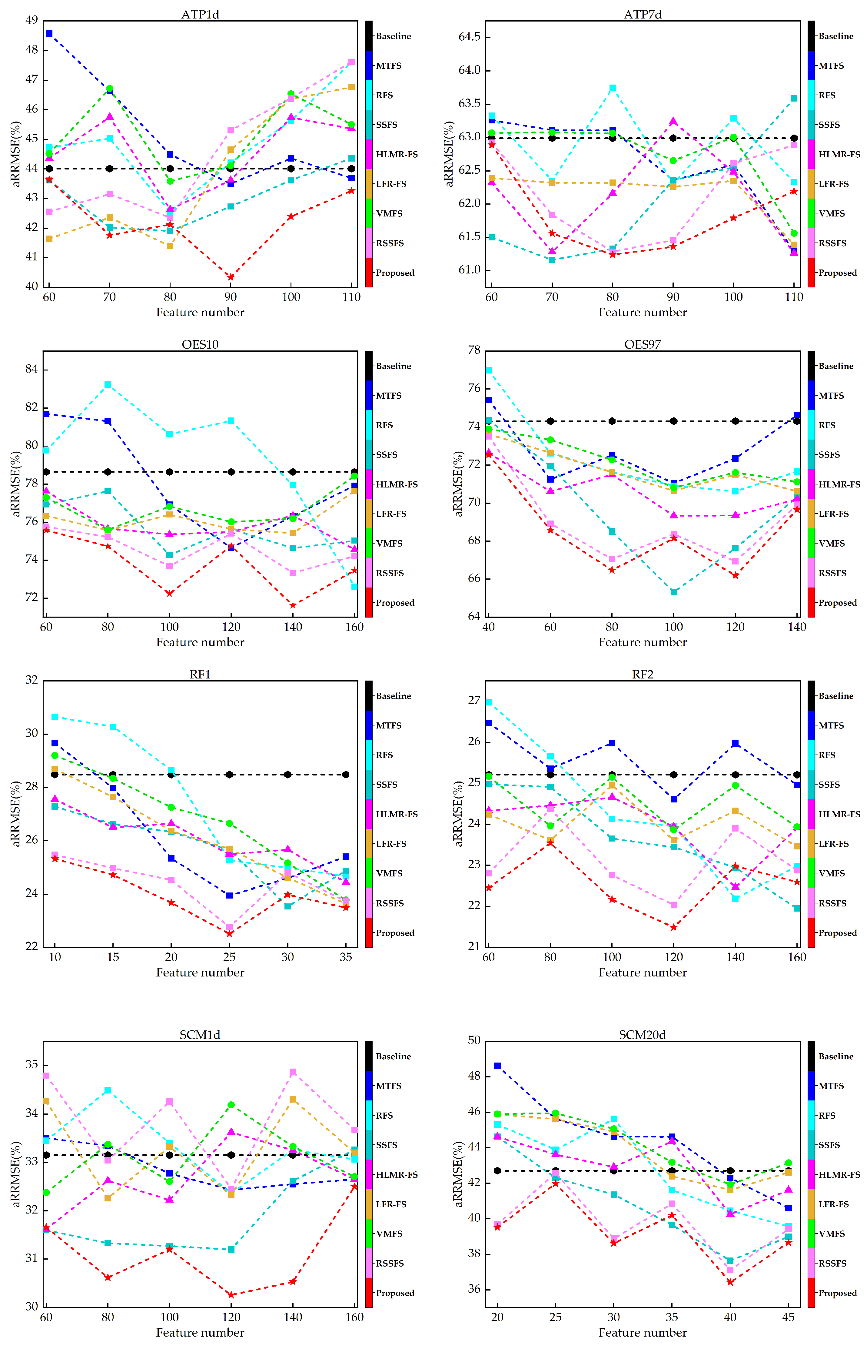
6.3. Evaluation Metrics

Two evaluation metrics are employed in experiment, including average Correlation Coefficient (aCC) and average Relative Root Mean Squared Error (aRRMSE) [47]. The definition of aCC is as follows,

$$aCC=\frac{1}{q}\sum _{i=1}^q\frac{{\sum }_{j=1}^{N_{test}}\left(y_i^{\left(j\right)}-{\overline{y}}_i\right)\left({\widehat{y}}_i^{\left(j\right)}-{\tilde{y}}_i\right)}{\sqrt{{\sum }_{j=1}^{N_{test}}{\left(y_i^{\left(j\right)}-{\overline{y}}_i\right)}^2{\sum }_{j=1}^{N_{test}}{\left({\widehat{y}}_i^{\left(j\right)}-{\tilde{y}}_i\right)}^2}}$$

(46)

where $y_i^{\left(j\right)}$ and ${\widehat{y}}_i^{\left(j\right)}$ are the real and predicted values of the jth sample on the target i, ${\overline{y}}_i$ and ${\tilde{y}}_i$ are the mean of true value and the predicted value on target i over the test set, respectively. Likewise, the formula for aRRMSE is given:

$$aRRMSE=\frac{1}{q}\sum _{i=1}^q\sqrt{\frac{{\sum }_{j=1}^{N_{test}}{\left(y_i^{\left(j\right)}-{\widehat{y}}_i^{\left(j\right)}\right)}^2}{{\sum }_{j=1}^{N_{test}}{\left(y_i^{\left(j\right)}-{\mathbf{y}}_i\right)}^2}}$$

(47)

where ${\mathbf{y}}_i$ is the average value of the training samples on the ith target.

6.4. Results on the Data Sets

Figure 1 and Figure 2 show the aRRMSE and aCC values for different MTFS methods on different data sets, respectively. For ATP1d and ATP7d, we choose 60, 70, 80, 90, 100, 110 features. For OES10, RF2 and SCM1d, we choose 60, 70, 80, 90, 100 and 110 features. For OES97, we choose 40, 60, 80, 100, 120 and 140 features. For RF1, we choose 10, 15, 20, 25, 30 and 35 features. For SCM20d, we choose 20, 25, 30, 35, 40 and 45 features.

Meanwhile, the best aCC and aRRMSE values of compared MTFS methods on various datasets are ranked, and the average rank of different methods on all datasets is calculated. The Friedman test [50] with the significant level $\alpha =0.05$ is employed, and we utilize Bonferroni-Dunn test [50] as the post hoc test to further analysis of the comparison. The critical difference (CD) is calculated to measure the difference between the proposed method and other algorithms. The calculation of CD is as follows:

$$CD=q_{\alpha }\sqrt{\frac{n\left(n+1\right)}{6T}}.$$

(48)

where n is the number of algorithms compared, and T is the number of datasets. At significance level $\alpha =0.05$, the corresponding $q_{\alpha }=3.73$, thus we have CD = 2.41 ($n=9,T=8$). Figure 3 and Figure 4 show the average ranks of different feature selection methods based on aRRMSE and aCC metrics.

Obviously, from Figure 1 and Figure 2, we can observe that for different data sets, selecting the correct number of feature subsets can achieve better results than the baseline, which indicates that for MTR problems, a practical feature selection method can not only improve the computational efficiency of the model but also improve the comprehensive performance of the model on different targets. Furthermore, the regression performance does not necessarily improve as the size of the selected features increases. On the contrary, in most cases, such as OES97, RF1, SCM20d, etc., the performance decreases as the number of selected features increases, indicating the presence of redundant or irrelevant features in the original feature set may significantly reduce the performance of regression.

For most cases, SSFS, HLMR-FS and the proposed method can obtain a lower aRRMSE and higher aCC than MTFS, RFS and VMFS. It shows that the performance of MTFS can be improved via a low-rank constraint. The proposed method not only considers the structural information of different samples in feature space but also uses the intrinsic correlation information between targets to improve the performance of MTFS. Furthermore, the proposed method can outperform the baseline in most cases, regardless of the number of features. It indicates that the proposed method can effectively alleviate the influence of redundant features, thereby maintaining outstanding performance on the selected subset even if some redundant features are included.

6.5. Effect of Low-Rank Constraint

We also investigate the influence of different ranks over different data sets, set $r=1,2,\dots ,q$. The performance when $r=q$ is taken as the performance of the algorithm at full rank, on account of the condition $r\le min\left\{d,q\right\}$. The number of input features d in the adopted data set is much larger than q, so the corresponding rank value of the regression matrix at full rank is q. We set $r=\left\{1,2,\dots ,6\right\}$ in the ATP1d; $r=\left\{1,2,\dots ,16\right\}$ in the OES10; $r=\left\{1,2,\dots ,8\right\}$ in the RF1; $r=\left\{1,2,\dots ,16\right\}$ in the SCM1d. By setting different values of r to impose low-rank constraints on $\mathbf{A}$ and $\mathbf{B}$. The fluctuations of aRRMSE and aCC values of the algorithm with $\alpha$ fixed are shown in Figure 5.

From Figure 5, it is evident that performance of the proposed method can be effectively improved by choosing the appropriate rank value for different data sets. In addition, most of the rank values in different data sets are better than the performance at full rank, which indicates that the regression matrix can decouple the inter-features and inter-target correlation via embedding the latent space of different dimensions, and it is beneficial to improve the regression performance and robustness of the model.

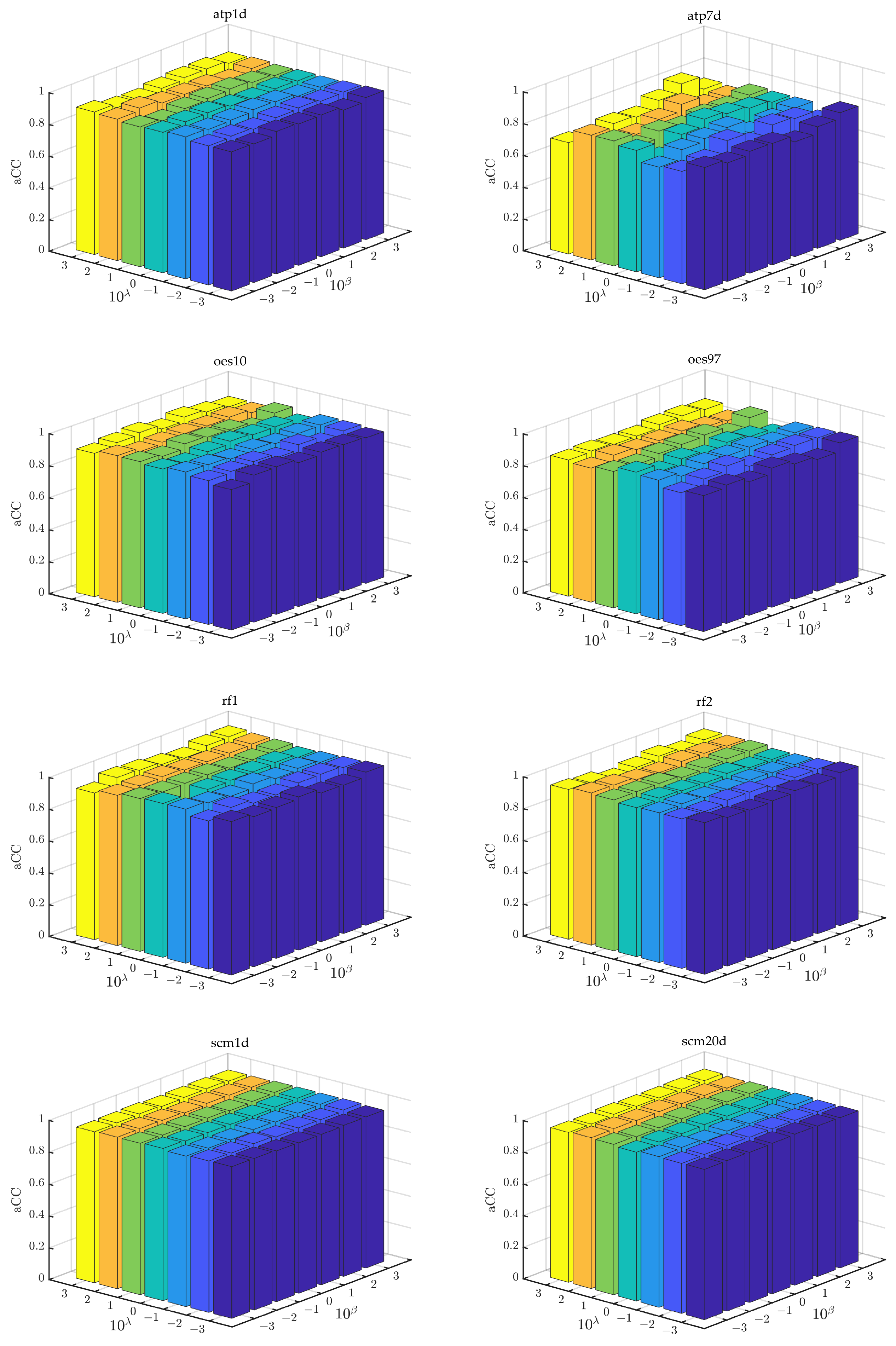
6.6. Parameter Sensitivity

In this section, we further perform sensitivity analysis on different parameters in the proposed feature selection method. Since there is a closed-form solution for $\gamma$, we focus on sensitivity analysis for the regularization parameters $\alpha$, $\lambda$ and $\beta$. First of all, we tuned the parameter $\alpha$ within the range of $\left\{{10}^{-3},{10}^{-2},\dots ,{10}^3\right\}$ with $\lambda =0.01$ and $\beta =0.01$. Likewise, we tuned parameters $\lambda$ and $\beta$ in $\left\{{10}^{-3},{10}^{-2},\dots ,{10}^3\right\}$ with $\alpha =0.1$, and the results are shown in Figure 6 and Figure 7.

In Figure 6, we can see that the variation of the parameter $\alpha$ will bring a certain degree of fluctuation in the model performance with $\lambda$ and $\beta$ fixed, which indicates that the proposed method is sensitive to $\alpha$. Hence, parameter $\alpha$ is vital to determine the performance of the proposed method. From Figure 7, it can be seen that the changes in model performance after changes in parameters $\lambda$ and $\beta$ in ranges are not as significant as that of parameter $\alpha$. However, properly tuning parameters $\lambda$ and $\beta$ can still improve the performance.

6.7. Convergence Study

We also plot the convergence curves of the objective function value of Equation (12) when the algorithm is updated iteratively on different data sets. As shown in Figure 8, it can be observed that ATP1d, ATP7d and RF1 can converge to the optimum within 20 iterations. The rest of the datasets can converge within 30 iterations, and the objective function converges quickly in the first few iterations. It indicates that the proposed alternating optimization algorithm can efficiently converge to the global optimum. Moreover, the monotone decrease of the objection function value demonstrates that the proposed problem can converge well. It confirms the effectiveness of the alternating optimization algorithm in addressing the proposed problem.

7. Conclusions

This paper has proposed a novel MTFS method based on adaptive graph learning and global target correlations to perform feature selection in MTR problem. Considering the existence of feature redundancy and noise in the original data, adaptive graph learning based on the sample local structure is introduced. Meanwhile, a manifold regularizer based on the target correlations is constructed to explore the inter-target correlation, which enables the regression matrix to consider the correlation between targets in the sparse and low-rank learning process. Finally, an alternating optimization algorithm is proposed to solve the objective function of the MTFS problem, and the convergence of the algorithm is demonstrated both theoretically and empirically. Through extensive experiments, it is demonstrated that the proposed method has superior performance compared with other mainstream embedding MTFS algorithms. The proposed method can effectively select features for MTR data, and then improve the efficiency and accuracy of MTR modelling.

In the future, we will extend the proposed method to cope with the semi-supervised and unsupervised feature selection tasks in MTR scenarios, we will try to introduce more manifold constraints and low-rank structures to the feature selection problem of MTR and test its performance and we will also explore whether it can solve the feature selection problem in multi-task learning and MLC.

References

1. Li, H.; Zhang, W.; Chen, Y.; Guo, Y.; Li, G.-Z.; Zhu, X. A novel multi-target regression framework for time-series prediction of drug efficacy. Sci. Rep. 2017, 7, 40652. [Google Scholar] [CrossRef] [PubMed]
2. Kocev, D.; Džeroski, S.; White, M.D.; Newell, G.R.; Griffioen, P. Using single- and multi-target regression trees and ensembles to model a compound index of vegetation condition. Ecol. Model. 2009, 220, 1159–1168. [Google Scholar] [CrossRef]
3. Sicki, D.M. Multi-target tracking using multiple passive bearings-only asynchronous sensors. IEEE Trans. Aerosp. Electron. Syst. 2008, 44, 1151–1160. [Google Scholar]
4. He, D.; Sun, S.; Xie, L. Multi-Target Regression Based on Multi-Layer Sparse Structure and Its Application in Warships Scheduled Maintenance Cost Prediction. Appl. Sci. 2023, 13, 435. [Google Scholar] [CrossRef]
5. Zhen, X.; Islam, A.; Bhaduri, M.; Chan, I.; Li, S. Descriptor Learning via Supervised Manifold Regularization for Multi-output Regression. IEEE Trans. Neural Netw. Learn. Syst. 2017, 28, 2035–2047. [Google Scholar] [PubMed]
6. Wang, X.; Zhen, X.; Li, Q.; Shen, D.; Huang, H. Cognitive Assessment Prediction in Alzheimer’s Disease by Multi-Layer Multi-Target Regression. Neuroinformatics 2018, 16, 285–294. [Google Scholar] [CrossRef] [PubMed]
7. Ghosn, J.; Bengio, Y. Multi-task learning for stock selection. In Proceedings of the 9th Advances in Neural Information Processing Systems, Denver, CO, USA, 2–5 December 1996; pp. 946–952. [Google Scholar]
8. Chen, B.J.; Chang, M.W. Load forecasting using support vector Machines: A study on EUNITE competition 2001. IEEE Trans. Power Syst. 2004, 19, 1821–1830. [Google Scholar] [CrossRef]
9. Cai, J.; Luo, J.; Wang, S.; Yang, S. Feature selection in machine learning: A new perspective. Neurocomputing 2018, 300, 70–79. [Google Scholar] [CrossRef]
10. Dinov, I.D. Variable/feature selection. In Data Science and Predictive Analytics: Biomedical and Health Applications Using R; Springer International Publishing: Cham, Switzerland, 2018; pp. 557–572. [Google Scholar]
11. Sechidis, K.; Spyromitros-Xioufis, E.; Vlahavas, I. Information Theoretic Multi-Target Feature Selection via Output Space Quantization. Entropy 2019, 21, 855. [Google Scholar] [CrossRef]
12. He, X.; Deng, C.; Niyogi, P. Laplacian Score for Feature Selection. In Proceedings of the Advances in Neural Information Processing Systems, Vancouver, BC, Canada, 5–8 December 2005; Volume 18. [Google Scholar]
13. Sechidis, K.; Brown, G. Simple strategies for semi-supervised feature selection. Mach. Learn. 2018, 107, 357–395. [Google Scholar] [CrossRef]
14. Kohavi, R.; John, G.H. Wrappers for feature subset selection. Artif. Intell. 1997, 97, 273–324. [Google Scholar] [CrossRef]
15. Tang, C.; Liu, X.; Li, M.; Wang, P.; Chen, J.; Wang, L.; Li, W. Robust unsupervised feature selection via dual self-representation and manifold regularization. Knowl.-Based Syst. 2018, 145, 109–120. [Google Scholar] [CrossRef]
16. Nouri-Moghaddam, B.; Ghazanfari, M.; Fathian, M. A novel multi-objective forest optimization algorithm for wrapper feature selection. Expert Syst. Appl. 2021, 175, 114737. [Google Scholar] [CrossRef]
17. Spyromitros-Xioufis, E.; Tsoumakas, G.; Groves, W.; Vlahavas, I. Multi-Label Classification Methods for Multi-Target Regression; Cornell University Library: Ithaca, NY, USA, 2014. [Google Scholar]
18. Spyromitros-Xioufis, E.; Tsoumakas, G.; Groves, W.; Vlahavas, I. Multi-target regression via input space expansion: Treating targets as inputs. Mach. Learn. 2016, 104, 55–98. [Google Scholar] [CrossRef]
19. Tsoumakas, G.; Spyromitros-Xioufis, E.; Vrekou, A.; Vlahavas, I. Multi-Target Regression via Random Linear Target Combinations; Springer: Berlin/Heidelberg, Germany, 2014; pp. 225–240. [Google Scholar]
20. Zhu, Y.; Kwok, J.T.; Zhou, Z.H. Multi-Label Learning with Global and Local Label Correlation. IEEE Trans. Knowl. Data Eng. 2018, 30, 1081–1094. [Google Scholar] [CrossRef]
21. Zhu, X.; Zhang, S.; Hu, R.; Zhu, Y.; Song, J. Local and Global Structure Preservation for Robust Unsupervised Spectral Feature Selection. IEEE Trans. Knowl. Data Eng. 2018, 30, 517–529. [Google Scholar] [CrossRef]
22. Huang, Y.; Shen, Z.; Cai, F.; Li, T.; Lv, F. Adaptive graph-based generalized regression model for unsupervised feature selection. Knowl.-Based Syst. 2021, 227, 107156. [Google Scholar] [CrossRef]
23. Zhen, X.; Yu, M.; He, X.; Li, S. Multi-Target Regression via Robust Low-Rank Learning. IEEE Trans. Pattern Anal. Mach. Intell. 2018, 40, 497–504. [Google Scholar] [CrossRef]
24. Zhen, X.; Yu, M.; Zheng, F.; Nachum, I.B.; Bhaduri, M.; Laidley, D.; Li, S. Multitarget Sparse Latent Regression. IEEE Trans. Neural Netw. Learn. Syst. 2018, 29, 1575–1586. [Google Scholar] [CrossRef]
25. Yang, J.; Zhang, D.; Yang, J.Y.; Niu, B. Globally Maximizing, Locally Minimizing: Unsupervised Discriminant Projection with Applications to Face and Palm Biometrics. IEEE Trans. Pattern Anal. Mach. Intell. 2007, 29, 650–664. [Google Scholar] [CrossRef]
26. Hashemi, A.; Dowlatshahi, M.B.; Nezamabadi-pour, H. VMFS: A VIKOR-based multi-target feature selection. Expert Syst. Appl. 2021, 182, 115224. [Google Scholar] [CrossRef]
27. Petkovi, M.; Kocev, D.; Deroski, S. Feature ranking for multi-target regression. Mach. Learn. 2020, 109, 1179–1204. [Google Scholar] [CrossRef]
28. Masmoudi, S.; Elghazel, H.; Taieb, D.; Yazar, O.; Kallel, A. A machine-learning framework for predicting multiple air pollutants’ concentrations via multi-target regression and feature selection. Sci. Total. Environ. 2020, 715, 136991. [Google Scholar] [CrossRef] [PubMed]
29. Yuan, H.; Zheng, J.; Lai, L.L.; Tang, Y.Y. Sparse structural feature selection for multitarget regression. Knowl.-Based Syst. 2018, 160, 200–209. [Google Scholar] [CrossRef]
30. Zhang, S.; Yang, L.; Li, Y.; Luo, Y.; Zhu, X. Low-Rank Feature Reduction and Sample Selection for Multi-output Regression; Springer International Publishing: Cham, Switzerland, 2016. [Google Scholar]
31. Fan, Y.; Chen, B.; Huang, W.; Liu, J.; Weng, W.; Lan, W. Multi-label feature selection based on label correlations and feature redundancy. Knowl.-Based Syst. 2022, 241, 108256. [Google Scholar] [CrossRef]
32. Xu, J.; Liu, J.; Yin, J.; Sun, C. A multi-label feature extraction algorithm via maximizing feature variance and feature-label dependence simultaneously. Knowl.-Based Syst. 2016, 98, 172–184. [Google Scholar] [CrossRef]
33. Samareh-Jahani, M.; Saberi-Movahed, F.; Eftekhari, M.; Aghamollaei, G.; Tiwari, P. Low-Redundant Unsupervised Feature Selection based on Data Structure Learning and Feature Orthogonalization. Expert Syst. Appl. 2024, 240, 122556. [Google Scholar] [CrossRef]
34. Ma, J.; Xu, F.; Rong, X. Discriminative multi-label feature selection with adaptive graph diffusion. Pattern Recognit. 2024, 148, 110154. [Google Scholar] [CrossRef]
35. Zhang, R.; Zhang, Y.; Li, X. Unsupervised feature selection via adaptive graph learning and constraint. IEEE Trans. Neural Netw. Learn. Syst. 2020, 33, 1355–1362. [Google Scholar] [CrossRef]
36. Zhu, X.; Zhang, S.; Zhu, Y.; Zhu, P.; Gao, Y. Unsupervised spectral feature selection with dynamic hyper-graph learning. IEEE Trans. Knowl. Data Eng. 2020, 34, 3016–3028. [Google Scholar] [CrossRef]
37. You, M.; Yuan, A.; He, D.; Li, X. Unsupervised feature selection via neural networks and self-expression with adaptive graph constraint. Pattern Recognit. 2023, 135, 109173. [Google Scholar] [CrossRef]
38. Acharya, D.B.; Zhang, H. Feature Selection and Extraction for Graph Neural Networks. In Proceedings of the 2020 ACM Southeast Conference (ACM SE ’20), Tampa, FL, USA, 2–4 April 2020; Association for Computing Machinery: New York, NY, USA, 2020; pp. 252–255. [Google Scholar] [CrossRef]
39. Chen, L.; Huang, J.Z. Sparse Reduced-Rank Regression for Simultaneous Dimension Reduction and Variable Selection. J. Am. Stat. Assoc. 2012, 107, 1533–1545. [Google Scholar] [CrossRef]
40. Liu, G.; Lin, Z.; Yan, S.; Sun, J.; Yu, Y.; Ma, Y. Robust Recovery of Subspace Structures by Low-Rank Representation. IEEE Trans. Pattern Anal. Mach. Intell. 2013, 35, 171–184. [Google Scholar] [CrossRef] [PubMed]
41. Doquire, G.; Verleysen, M. A graph Laplacian based approach to semi-supervised feature selection for regression problems. Neurocomputing 2013, 121, 5–13. [Google Scholar] [CrossRef]
42. He, X.; Niyogi, P. Locality preserving projections. In Proceedings of the Advances in Neural Information Processing Systems, Vancouver, BC, USA, 8–13 December 2003; Volume 16. [Google Scholar]
43. Wang, H.; Yang, Y.; Liu, B. GMC: Graph-Based Multi-View Clustering. IEEE Trans. Knowl. Data Eng. 2020, 32, 1116–1129. [Google Scholar] [CrossRef]
44. Liu, J.; Ji, S.; Ye, J. Multi-task feature learning via efficient 2,1-norm minimization. In Proceedings of the Conference on Uncertainty in Artificial Intelligence, Montreal, QC, Canada, 18–21 June 2009; pp. 339–348. [Google Scholar]
45. Tsoumakas, G.; Spyromitros-Xioufis, E.; Vilcek, J. MULAN: A Java library for multi-label learning. J. Mach. Learn. Res. 2011, 12, 2411–2414. [Google Scholar]
46. Nie, F.; Huang, H.; Cai, X.; Ding, C. Efficient and Robust Feature Selection via Joint 2,1-Norms Minimization. In Proceedings of the Neural Information Processing Systems (NIPS), Vancouver, BC, USA, 6–9 December 2010; pp. 1813–1821. [Google Scholar]
47. Borchani, H.; Varando, G.; Bielza, C.; Larrañaga, P. A survey on multi-output regression. WIREs Data Min. Knowl. Discov. 2015, 5, 216–233. [Google Scholar] [CrossRef]
48. Sheikhpour, R.; Gharaghani, S.; Nazarshodeh, E. Sparse feature selection in multi-target modeling of carbonic anhydrase isoforms by exploiting shared information among multiple targets. Chemom. Intell. Lab. Syst. 2020, 200, 104000. [Google Scholar] [CrossRef]
49. Shawe-Taylor, J.; Cristianini, N. Kernel Methods for Pattern Analysis; Cambridge University Press: Cambridge, UK, 2004. [Google Scholar]
50. Demšar, J.; Schuurmans, D. Statistical comparisons of classifiers over multiple data sets. J. Mach. Learn. Res. 2006, 7, 1–30. [Google Scholar]
Figure 1. aRRMSE results compared with compared methods under different number of selected features.
Mathematics 12 00372 g001
Figure 2. aCC results compared with state-of-the-art methods under different number of selected features.
Mathematics 12 00372 g002
Figure 3. Average rank of different feature selection methods based on aRRMSE under Bonferroni–Dunn test.
Mathematics 12 00372 g003
Figure 4. Average rank of feature selection methods based on aCC under Bonferroni–Dunn test.
Mathematics 12 00372 g004
Figure 5. Performance of feature selection methods under different low-rank constraints.
Mathematics 12 00372 g005
Figure 6. Sensitivity analysis of the parameter α with λ and β fixed.
Mathematics 12 00372 g006
Figure 7. Sensitivity analysis of the parameter λ and β with α fixed.
Mathematics 12 00372 g007
Figure 8. Convergence curves of the proposed method under different data sets.
Mathematics 12 00372 g008