Imposing Star-Shaped Hard Constraints on the Neural Network Output

Abstract

A problem of imposing hard constraints on the neural network output can be met in many applications. We propose a new method for solving this problem for non-convex constraints that are star-shaped. A region produced by constraints is called star-shaped when there exists an origin in the region from which every point is visible. Two tasks are considered: to generate points inside the region and on the region boundary. The key idea behind the method is to generate a shift of the origin towards a ray parameterized by the additional layer of the neural network. The largest admissible shift is determined by the differentiable Ray marching algorithm. This allows us to generate points which are guaranteed to satisfy the constraints. A more accurate modification of the algorithm is also studied. The proposed method can be regarded as a generalization of the methods for convex constraints. Numerical experiments illustrate the method by solving machine-learning problems. The code implementing the method is publicly available.

1. Introduction

Many machine-learning tasks solved by means of neural networks, for example, solvers of optimization problems, models generating images in a predefined region, control problems with actions in some interval, require the restriction of the neural network outputs by certain constraints. The restrictions imply that outputs of a neural network have to satisfy specified constraints.

The most existing approaches to construct a neural network with the output constraints are based on adding regularization terms to a loss function of the network to penalize constraint violations. However, the corresponding soft constraints only penalize their possible violation, but they do not guarantee that the constraints will be satisfied for a new example [1]. Another interesting approach is to modify the neural network to provide predictions within a set formed by the constraints. In this case, we have hard constraints which are satisfied for any input example during training and inference [2].

There are several approaches to impose hard constraints on the neural network outputs, for example, [2,3,4,5,6,7]. Most approaches consider the linear and convex hard constraints. One of the approaches to impose convex constraints was proposed in [8]. The key idea behind the method is to add a neural network layer which maps a latent vector to a point that is guaranteed to be inside a feasible set defined by the constraints. Following this method, we propose its extension, which allows us to consider the well-known type of non-convex constraints called the star-shaped constraints [9]. At that, the convex constraints can be regarded as a special case of constraints that can be used in the proposed method. To the best of our knowledge, at the moment, no approach is known that allows building layers of neural networks implementing the non-convex star-shaped constraints such that the optimization problem is not solved during the forward pass of the neural network.

The proposed method can be applied to solving optimization problems with arbitrary differentiable loss functions and with star-shaped constraints, to implementing generative models with constraints. It can be used when constraints are imposed on a predefined points or a subsets of points.

Our contributions can be summarized as follows:

• A problem of building a neural network with non-convex hard constraints on output vectors is formulated. The neural network consists of two parts. The first part is an arbitrary neural network that processes input data. The second part is a layer that implements the proposed method for restricting predictions by star-shape constraints.
• A method for non-convex constraints specification, inspired by constructive solid geometry in computer graphics, is proposed.
• A new neural network layer for implementing the hard constraints on star-shape domains is introduced.
• The proposed method is evaluated, confirming experimentally its properties.

The corresponding code implementing the proposed method is publicly available at https://github.com/NTAILab/star_hard_constraints (accessed on 25 November 2024).

The paper is organized as follows. Related work can be found in Section 2. The problem statement for constructing a neural network with outputs satisfying certain constraints for an arbitrary input vector is given in Section 3. Section 4 describes how to represent the star-shaped region as a combination of the set operations. The signed distance function used to represent non-convex sets is introduced in the same section. The general method for constructing a neural network with restricted output and its modification is provided in Section 5. An approach for applying the ray casting method for solving the stated problem is considered in Section 6. Numerical experiments illustrating the proposed method are provided in Section 7. Concluding remarks can be found in Section 8.

2. Related Work

It should be noted that a few machine-learning models implement hard constraints. Brosowsky et al. [5] proposed a neural network architecture which imposes linear hard constraints on the network output by using a linear combination of vertices of a polyhedron produced by the constraints with coefficients in the form of the softmax operation results. A limitation of the method is that only linear constraints are considered. Another limitation is that the method requires the enumeration of all vertices of a polyhedron produced by the linear constraints, whose number may be very large. Frerix et al. [2] proposed an approach for solving problems with conical constraints of the form $Ax\le 0$. According to the approach, points are generated in the set produced by linear constraints $Ax\le 0$ by means of a set of rays. It is important to point out that the authors of [2] claim that the approach does not allow for efficient incorporation of constraints in some cases. Moreover, if the method is applied to non-conical constraints, then all vertices of the set have to be considered. Another approach specifically designed for solving constrained optimization problems is provided by Donti et al. [6]. The approach tries to incorporate equality and inequality constraints into the learning-based optimization algorithms. However, its performance heavily relies on the training process and the chosen model architecture. A method for solving optimization problem with linear constraints is also presented in [10]. The method allows solving the optimization problems only with linear constraints and may also require significant computational resources. An RL algorithm designed to enforce affine hard constraints in a task of the robot policy learning was proposed in [11]. An outstanding framework to impose hard convex constraints on the neural network outputs called RAYEN was presented in [7]. It supports any combination of linear and convex quadratic inequality constraints. An interesting approach for solving quadratic optimization problems with linear constraints posed on the neural network outputs was proposed in [4]. Agrawal et al. [3] presented a similar approach based on adding a differentiable optimization layer to a neural network, which implements a projection operator to guarantee that the neural network output satisfies constraints. However, according to this approach, convex optimization problems have to be solved for each forward pass. In [1], the authors show that imposing hard constraints can in fact be done in a computationally feasible way by using a Krylov subspace approach. Liu et al. [12] proposed a differentiable layer, named the differentiable Frank-Wolfe layer, using the well-known Frank-Wolfe method for solving constrained optimization problems without projections and Hessian matrix computations. Sun et al. [13] developed a new framework, named alternating differentiation, that differentiates convex optimization problems with polyhedral constraints in a fast and recursive way.

A number of approaches partially addressing the task of solving constrained optimization problems were considered in [14,15,16,17,18,19,20,21]. They are analyzed in survey papers [22,23]. At the same time, the aforementioned approaches solve optimization problems with linear or convex constraints, but they do not consider the non-convex star-shaped constraints.

3. The Problem Statement

A connected region is called star-shaped when it contains a point from which every boundary point is visible. Formally, if the feasible set $\Omega \subset {\mathbb{R}}^n$ is the star-shaped region, then there exists a point $p\in {\mathbb{R}}^n$ such that every point $x\in \Omega$ can be represented as

$$x=p+\alpha ·r,$$

(1)

where r is a vector or a ray, $∥r∥=1$; $\alpha \in \mathbb{R}$ is a scale factor, and $\alpha \ge 0$.

The condition $p+\beta ·r\in \Omega$ is fulfilled for all $\beta \in \mathbb{R}$ such that $0\le \beta \le \alpha$, i.e., the entire segment belongs to the region:

$$\{p+\beta ·r\mid \beta \in \mathbb{R},0\le \beta \le \alpha \}\in \Omega .$$

(2)

The point p is called the origin. Let $\Omega$ be a star-shaped region specified by a set of constraints. The first goal is to construct a differentiable neural network layer with outputs, satisfying constraints for an arbitrary input vector:

$$f_{\Omega }:{\mathbb{R}}^d\mapsto \Omega$$

(3)

such that $f_{\Omega }$ is surjective.

The second goal is to build a surjective mapping $g_{\Omega }$ to the boundary of $\Omega$ denoted as $\partial \Omega$, i.e.,:

$$g_{\Omega }:{\mathbb{R}}^d\mapsto \partial \Omega .$$

(4)

It should be noted that, in practice, the precise mapping to the boundary cannot be constructed due to numerical errors, and, therefore, the second goal is to find an $ϵ$-accurate mapping to the boundary such that

$$\forall z\in {\mathbb{R}}^d\exists b\in \partial \Omega (∥g_{\Omega }-b∥<ϵ).$$

(5)

4. Region Definition as a Signed Distance Function

In the case of convex constraints, the natural region definition can be formulated as a system of inequality constraints, which is equivalent to an intersection of convex regions. For star-shaped non-convex regions, not only can the intersection operation be used, but also union, subtraction, and so on. It is worth mentioning that the star-shape property is not closed under union and even intersection operations, meaning that an intersection of two star-shaped regions can be not star-shaped. Therefore, we use a general scheme for defining non-convex constraints, because no specific scheme for star-shaped regions can be implemented.

For defining a non-convex domain, we follow the principle of constructive solid geometry, where a complex object is defined as a combination of set operators and geometric primitives, such as cuboids, spheres, hyperplanes, etc. The whole object can be seen as a tree, where internal nodes represent operators, edges connect operators with arguments to which they apply, and the leaf nodes are primitives.

We define a constraint tree as a graph whose nodes represent n-ary operators and edges connect the operators to their arguments. Leaf nodes in the tree correspond to primitives, and can be considered as 0-ary operators.

Basically, the non-convex region $\Omega \subset {\mathbb{R}}^d$ can be represented as a composition of the union and intersection operations over some sets, recursively represented in the same way, and convex primitives. For example:

$$\Omega =(\mathrm{Sphere}\cap \mathrm{Cube})\cup \mathrm{Plane},$$

(6)

or in another form:

$$\Omega =\mathrm{Union}\left(\mathrm{Intersection}\right(\mathrm{Sphere},\mathrm{Cube}),\mathrm{Plane}).$$

(7)

However, some more complex scenarios require additional operators, such as the set difference “∖”, especially, when the set of primitives is limited to convex primitives. Therefore, we consider different sets of operators, starting from the simplest one to the general case:

• Only the intersection operator “∩” can be considered, which is equivalent to the system of constraints:

  $$\left\{\begin{array}{c}{h}_1\left(x\right)\le 0,\\ \dots \\ h_k\left(x\right)\le 0,\end{array}\right.$$

  (8)

  where each constraint $h_i\left(x\right)\le 0$ represents a primitive, e.g., a plane. In the case of convex primitives, it leads to a convex domain.
• The intersection “∩” and union “∪” operators can be studied. A computationally simple algorithm for constructing non-convex sets with the above operators is described below in detail.
• The complete set of operators includes the intersection and union operators as well as the set difference “∖” operator.

A connected non-convex region can be defined in one of three ways described above. Intuitively, the simpler the definition is, the more effective the algorithm that can be implemented. For example, for the first above case and linear constraints, the algorithm is linear and can be reduced to the ray-hyperplane intersection and to the minimum calculations [8]. For other cases, two different methods are considered further.

In a general case, a constraint tree for the region $\Omega$ can be associated with a signed distance function (SDF) considered in [24]. Formally, it is defined as a function $\sigma \left(x\right)$ that measures a distance to the set boundary $\partial \Omega$ multiplied by $-1$ in a case when an input point lies inside the $\Omega$:

$$\begin{array}{cc}\hfill x& \in \Omega \iff \sigma \left(x\right)\le 0,\hfill \\ \hfill x& \in \partial \Omega \iff \sigma \left(x\right)=0.\hfill \end{array}$$

(9)

If $x\notin \Omega$, then the SDF value is positive and coincides with the distance to $\partial \Omega$, i.e., the following holds

$$x\notin \Omega \iff \sigma \left(x\right)>0.$$

Each set operator in a constraint tree can be translated into the SDF operator:

$$x\in \Omega ={\Omega }_1•{\Omega }_2\iff \sigma \left(x\right)=q_{•}({\sigma }_1\left(x\right),{\sigma }_2\left(x\right)),$$

(10)

where • represents a set operator which is defined for different values as:

• $q_{\cup }(a,b)=\min \{a,b\}$;
• $q_{\cap }(a,b)=\max \{a,b\}$;
• $q_{\setminus }(a,b)=\max \{a,-b\}$.

A unary inverse operator is

$$x\in \Omega =U\setminus {\Omega }_1\iff \sigma \left(x\right)=-{\sigma }_1\left(x\right).$$

(11)

It can be seen from the above that the SDF can be used to represent non-convex sets and to implement the set operations. The sign of the SDF can be used to check whether a point belongs to the region $\Omega$ ot not.

The idea behind the SDF usage is to represent both convex and non-convex regions in the form of a function in a computationally simple way because the set operations are rather simple.

5. General Method

We propose a neural network consisting of two parts. The first part is an arbitrary neural network, which processes input data that is specific to a concrete application problem, for example, it can be a convolutional neural network for the image inputs. The second part is a layer whose outputs are guaranteed to satisfy star-shape constraints (see Figure 1). Let us describe this layer in detail.

Suppose that $p_{\Omega }$ is the origin of $\Omega$, which is star-shaped, closed, and has a non-zero volume. Then, by definition, every point $x\in \Omega$ can be parameterized by a pair $(\alpha ,r)$, such that $p_{\Omega }+\alpha ·r=x$. The main idea behind the method is to use this parameterization to construct points inside $\Omega$, so the corresponding output of the neural network layer (see Section 3) is calculated as:

$$f_{\Omega }\left(z\right)=p_{\Omega }+{\alpha }_{\theta }\left(z\right)·r_{\theta }\left(z\right),$$

(12)

where $\parallel r_{\theta }\left(z\right)\parallel =1$, and ${\alpha }_{\theta }\left(z\right)$ and $r_{\theta }\left(z\right)$ are outputs of neural networks with parameters $\theta$, which map an input to the step size and the ray direction, respectively. The step size ${\alpha }_{\theta }\left(z\right)$ should not violate constraints along the ray $r_{\theta }\left(z\right)$:

$$0\le {\alpha }_{\theta }\left(z\right)\le \underset{\alpha }{\sup }\{\alpha \mid p_{\Omega }+\alpha ·r_{\theta }\left(z\right)\in \Omega \}.$$

(13)

Obviously, the upper boundary of ${\alpha }_{\theta }\left(z\right)$ depends on the ray direction $r_{\theta }\left(z\right)$. Let us denote the above supremum as ${\alpha }^{*}\left(r_{\theta }\left(z\right)\right)$. The second goal can be achieved by constructing the neural network layer as:

$$g_{\Omega }\left(z\right)=p_{\Omega }+{\alpha }^{*}\left(r_{\theta }\left(z\right)\right)·r_{\theta }\left(z\right).$$

(14)

The function $g_{\Omega }\left(z\right)$ can be regarded as a neural network with parameters $\theta$.

The mapping to the boundary $g_{\Omega }$ can be used to construct the neural network $f_{\Omega }$ with parameters $\theta$ in two ways described below.

5.1. Ray and Scale Approach

First, a point inside the region $\Omega$ can be represented as a convex combination of the origin $p_{\Omega }$ and some point on the boundary. Hence, we can write the following expression for $f_{\Omega }\left(z\right)$ in terms of the neural networks described above:

$$\begin{array}{cc}\hfill f_{\Omega }\left(z\right)& =(1-\gamma )·p_{\Omega }+\gamma ·g_{\theta }\left(z\right)\hfill \\ \hfill & =p_{\Omega }+\gamma ·{\alpha }^{*}\left(r_{\theta }\left(z\right)\right)·r_{\theta }\left(z\right),\gamma \in [0,1].\hfill \end{array}$$

(15)

Therefore, ${\alpha }_{\theta }\left(z\right)=\gamma ·{\alpha }^{*}\left(r_{\theta }\left(z\right)\right)$ can be used to generate points in the region interior. The mapping $f_{\Omega }$ should be surjective, so $\gamma$ necessarily should be a function of z. For example, in the implementation, ${\gamma }_{\theta }\left(z\right)$ can be the output of a neural network with the sigmoid activation function at the last layer.

5.2. Extended Space Approach

The second way to construct $f_{\Omega }$ by using $g_{\tilde{\Omega }}$ is to increase the output space dimensionality by one, obtaining the region $\tilde{\Omega }\subset {\mathbb{R}}^{n+1}$, which is described below, and then to find a boundary point and a project back to the original space $\Omega \subset {\mathbb{R}}^n$. We can use an arbitrary definition of $\tilde{\Omega }$, when two conditions are satisfied. First, the region $\tilde{\Omega }$ can be projected to the original region $\Omega$, i.e., the 0-th component represents the extra dimension:

$$\{x\in {\mathbb{R}}^n|\exists {\xi }_0\in \mathbb{R}:{({\xi }_0,x_1,\dots ,x_n)}^T\in \tilde{\Omega }\}=\Omega .$$

(16)

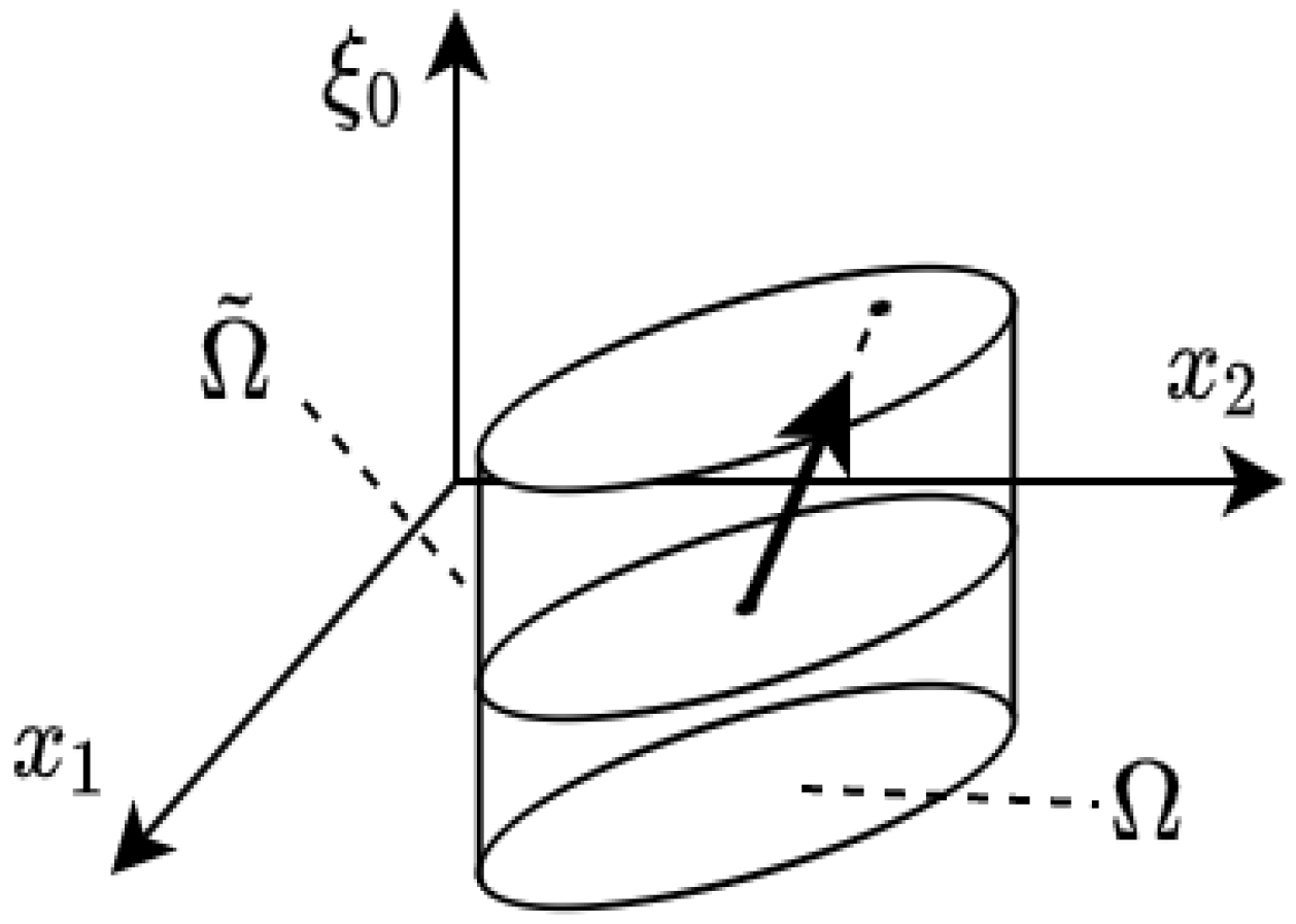
Second, the region $\tilde{\Omega }$ should be also star-shaped, closed, and with a non-zero volume. A straightforward example (see Figure 2), satisfying the above two conditions, is a closed cylinder defined as:

$$\tilde{\Omega }=\left\{\xi \in {\mathbb{R}}^{n+1}|{\xi }_0\in [-\nu ,\nu ],{({\xi }_1,\dots ,{\xi }_n)}^T\in \Omega \right\},$$

(17)

where $\nu \in \mathbb{R}$ and $\nu >0$.

Using the set $\tilde{\Omega }$, the mapping to the region $\Omega$ interior can be constructed from $g_{\tilde{\Omega }}$ in the following way:

$$f_{\Omega }\left(z\right)=\Pi \left[g_{\tilde{\Omega }}\left(z\right)\right],$$

(18)

where the projection $\Pi$ is carried out by discarding 0-th component:

$$\Pi \left[{({\xi }_0,{\xi }_1,\dots ,{\xi }_n)}^T\right]={({\xi }_1,\dots ,{\xi }_n)}^T.$$

(19)

Since $\tilde{\Omega }$ can be represented as an intersection of linear constraints on ${\zeta }_0$ and the original domain

$$\tilde{\Omega }=\{\zeta \in {\mathbb{R}}^{n+1}|{({\zeta }_1,\dots ,{\zeta }_n)}^T\in \Omega \}\cap \{\zeta \in {\mathbb{R}}^{n+1}|{\zeta }_0\in [-\nu ,\nu ]\},$$

(20)

then SDF for $\tilde{\Omega }$ can be inferred from ${\sigma }_{\Omega }\left(x\right)$ by applying the intersection operator on SDF:

$${\sigma }_{\tilde{\Omega }}\left(\tilde{x}\right)=\max \left\{{\sigma }_{\Omega }\left(x\right),{\tilde{x}}_0-\nu ,-\nu -{\tilde{x}}_0\right\}.$$

(21)

Therefore, an extended space does not have to be explicitly defined for estimating the SDF-based intersection point $\tilde{x}$ calculated as $g_{\tilde{\Omega }}\left(z\right)$ such that ${\sigma }_{\tilde{\Omega }}\left(\tilde{x}\right)=0$.

When the value of $\nu$ is large, the first term in the maximum (21), ${\sigma }_{\Omega }\left(x\right)$, will dominate, and points will concentrate at the boundary. This problem can be solved by taking $\nu$ as a function of $x,$ i.e., $\nu \left(x\right)$. A special case is when $\nu \left(x\right)=\left|{\sigma }_{\Omega }\left(x\right)\right|$, which allows avoiding manual tuning of $\nu$. The SDF with such values of $\nu$ is

$${\sigma }_{\tilde{\Omega }}\left(\tilde{x}\right)=\max \left\{{\sigma }_{\Omega }\left(x\right),{\tilde{x}}_0-\left|{\sigma }_{\Omega }\left(x\right)\right|,-\left|{\sigma }_{\Omega }\left(x\right)\right|-{\tilde{x}}_0\right\},$$

(22)

and it can be interpreted as a SDF of the union of spheres of radius $\left|{\sigma }_{\Omega }\left(x\right)\right|$ around every point of $\Omega$.

The main remaining question for implementing $f_{\Omega }$ and $g_{\Omega }$ is how to estimate the maximum allowable step size ${\alpha }^{*}\left(r\right)$ in a differentiable way.

5.3. Iterative Approach for Finding ${\alpha }^{*}\left(r\right)$

The most general approach of finding the maximum allowable step size ${\alpha }^{*}\left(r\right)$, which can be applied to an arbitrary constraint tree, is based on optimization of the SDF absolute value along the ray, and is usually called the ray marching algorithm. This algorithm was initially proposed in [25] for applying to the computer graphics field. It is not limited to the specific constraint tree structures or a narrow set of the set operations, and allows us to decide on the quality–performance trade-off. The algorithm is based on using the SDF value as a step size along the ray direction, which guarantees that the tracing path will not pass through the object boundary. It iteratively updates the intersection point estimate by moving it along the ray until $|{\sigma }_{\Omega }\left(x\right)|<\epsilon$. The iterative process can be described as follows:

$$\begin{array}{c}{\alpha }_0=0,\hfill \\ \hfill {\alpha }_i={\alpha }_{i-1}+\left|{\sigma }_{\Omega }(p_{\Omega }+{\alpha }_{i-1}·r)\right|,i=1,\dots ,M.\end{array}$$

(23)

The SDF function ${\sigma }_{\Omega }$ is computed by combining operators $q_{\cup },q_{\cap },q_{\setminus }$ in accordance with the constraint tree.

Gradient Estimation

Since ${\alpha }^{*}\left(r\right)$ depends on the ray direction, which is calculated as an output of the neural network $r_{\theta }\left(z\right)$, then we have to calculate gradient of ${\alpha }^{*}\left(r\right)$ to optimize parameters $\theta$ of the neural network. We consider two approaches to compute the partial derivative with respect to the ray direction vector:

• by differentiation through a sequence of iterations;
• by the implicit function differentiation.

The first approach is natural for neural networks. It is based on an automated differentiation algorithm and requires the calculation of the derivative of the SDF M times. The second approach, based on the implicit function, is much more computationally effective because it allows us to estimate the gradient at the intersection point in a single pass. The only limitation is that it assumes that the intersection point estimation is precise. Let us consider the second approach in detail. The step size ${\alpha }^{*}\left(r\right)$ is a function of r, such that there holds for all r:

$${\sigma }_{\Omega }\left(\chi (r,{\alpha }^{*}\left(r\right))\right)=0,$$

(24)

where $\chi$ is the layer that maps inputs onto $\partial \Omega$:

$$\chi (r,\alpha )=p_{\Omega }+\alpha ·r.$$

(25)

We have to find the derivative of $\chi$ with respect to r, for which partial derivatives ${\displaystyle \frac{\partial {\alpha }^{*}\left(r\right)}{\partial r_j}}$ are needed because of

$$\begin{array}{cc}\hfill {\displaystyle \frac{\partial {\left(\chi (r,{\alpha }^{*}\left(r\right))\right)}_i}{\partial r_j}}& ={\displaystyle \frac{\partial {\alpha }^{*}\left(r\right)}{\partial r_j}}{r}_i+{\alpha }^{*}\left(r\right){\displaystyle \frac{\partial r_i}{\partial r_j}}\hfill \\ \hfill & ={\displaystyle \frac{\partial {\alpha }^{*}\left(r\right)}{\partial r_j}}{r}_i+{\alpha }^{*}\left(r\right){\delta }_{ij},\hfill \end{array}$$

(26)

where $i,j\in \{1,\dots ,n\}$.

Let us define $g={\sigma }_{\Omega }\circ \chi$. If ${\displaystyle \frac{\partial g(r,\alpha )}{\partial \alpha }}\ne 0$, then we can apply the implicit function theorem [26]: there is a small neighborhood around $\alpha$, where the function ${\alpha }^{*}\left(r\right)$ exists such that $g(r,{\alpha }^{*}\left(r\right))=0$, and

$${\displaystyle \frac{\partial {\alpha }^{*}\left(r\right)}{\partial r_j}}=-{\displaystyle \frac{\partial g}{\partial r_j}}·{\left({\displaystyle \frac{\partial g(r,\alpha )}{\partial \alpha }}\right)}^{-1}.$$

(27)

The partial derivative of g at point $\alpha$ can be found analytically:

$${\displaystyle \frac{\partial g(r,\alpha )}{\partial \alpha }}={\left.\sum _{i=1}^d{\displaystyle \frac{\partial \sigma \left(\xi \right)}{\partial {\xi }_i}}\right|}_{\xi =x(r,\alpha )}·{\displaystyle \frac{\partial {\left(\chi (r,\alpha )\right)}_i}{\partial \alpha }}=r^T\nabla {\sigma }_{\Omega },$$

(28)

and the gradient of g at point $(r,\alpha )$, where $\alpha$ is constant, is:

$${\nabla }_{r}g=\nabla \left({\sigma }_{\Omega }(p_{\Omega }+\alpha ·r)\right)=\alpha ·\nabla {\sigma }_{\Omega }.$$

(29)

Therefore, the desired gradient is a scaled normal of the decision boundary:

$$\nabla {\alpha }^{*}\left(r\right)=-{\displaystyle \frac{\alpha }{r^T\nabla {\sigma }_{\Omega }}}·\nabla {\sigma }_{\Omega }.$$

(30)

When the denominator is zero, the decision boundary normal is orthogonal to the ray direction, and $\nabla {\alpha }^{*}$ can be set to zero too. Finally, a neural network with the proposed layer at the end is suitable for the gradient-based optimization or training. Indeed, if the ray direction function r is implemented as a neural network with the parameters $\theta$: $r_{\theta }\left(z\right)$, and some loss functional $l\left(x_{\theta }\left(z\right)\right)$ is defined, where $x_{\theta }\left(z\right)=\chi \left(r_{\theta }\left(z\right),{\alpha }^{*}\left(r_{\theta }\left(z\right)\right)\right)$, then the loss gradient over the vector of parameters can be found as:

$${\nabla }_{\theta }^{T}l={\nabla }_x^{T}l\left(x_{\theta }\left(z\right)\right){\mathbf{J}}_r\left(\chi (r,{\alpha }^{*}\left(r\right))\right){\mathbf{J}}_{\theta }\left(r_{\theta }\left(z\right)\right),$$

(31)

where the loss function gradient ${\nabla }_{x}l\left(x_{\theta }\left(z\right)\right)$ is known, ${\mathbf{J}}_{\theta }\left(r_{\theta }\left(z\right)\right)$ is found via automatic differentiation, and the Jacobian matrix of $\chi (r,{\alpha }^{*}\left(r\right))$ at r is of the form:

$$\begin{array}{cc}\hfill {\mathbf{J}}_r\left(\chi (r,{\alpha }^{*}\left(r\right))\right)& =(\nabla {\alpha }^{*}\left(r\right))r^T+{\alpha }^{*}\left(r\right)·I\hfill \\ \hfill & ={\displaystyle \frac{{\alpha }^{*}\left(r\right)}{r^T\nabla {\sigma }_{\Omega }}}·\left[r^T\nabla {\sigma }_{\Omega }·I-(\nabla {\sigma }_{\Omega })r^T\right].\hfill \end{array}$$

(32)

5.4. Modification

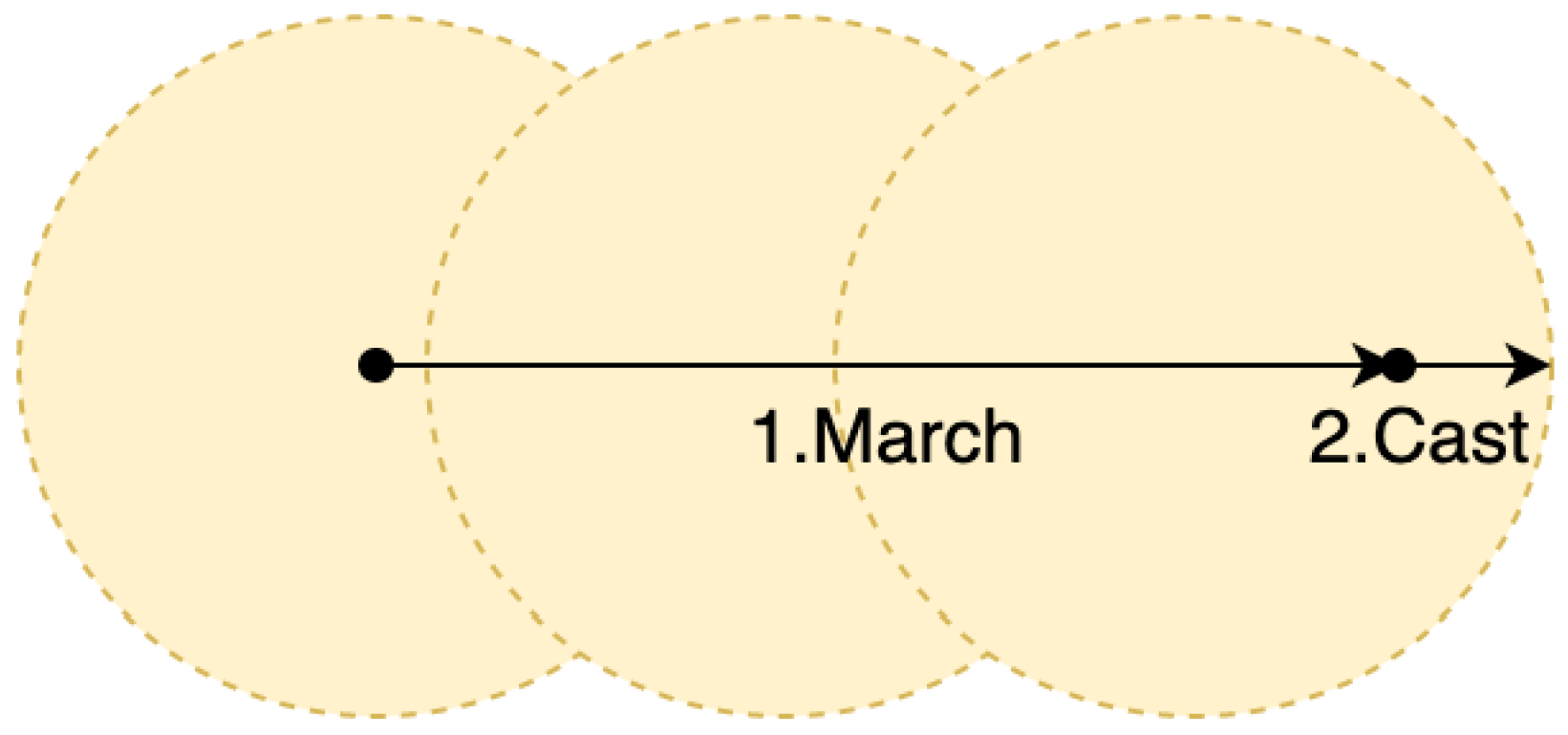
The above gradient estimation is exact when the iterative marching process converges exactly to the boundary point. It takes place in some cases, for example, when $\Omega$ is a sphere, or a hyperplane, and the ray direction is collinear with the hyperplane normal. In general, the iterative process with a finite number of steps can converge to a point which is $\epsilon$-close to the boundary. Hence, the proposed gradient estimation becomes less accurate. To increase the accuracy, a two-stage modification can be used (see Figure 3). At the first stage, the iterative marching process is used to find an intersection point approximation, which is $\epsilon$-close to the boundary, but is not exactly at it. At the second stage, the ray casting is applied from the approximate point to the closest primitive, determined at the SDF calculation. The required number of steps can be found in advance to guarantee $\epsilon$-accurate approximation, for which the ray casting produces correct results on the boundary.

If we define a set of the ray points that belong to the domain $\Omega$ as:

$$I_{\Omega }(x,r)=\left\{\alpha |{\sigma }_{\Omega }(x+\alpha ·r)\le 0,\alpha \ge 0\right\},$$

(33)

then the function $D_{\Omega }(x,r)$ determines a distance to the domain boundary along the ray:

$$D_{\Omega }(x,r)=\left\{\begin{array}{cc}\min I_{\Omega }(x,r),\hfill & I_{\Omega }(x,r)\ne Ø,\hfill \\ +\infty ,\hfill & \mathrm{otherwise}.\hfill \end{array}\right.$$

(34)

Formally, the modified algorithm has one additional step:

$${\alpha }_{M+1}={\alpha }_M+\underset{k}{\min }{D}_{{\Omega }_k}(x+{\alpha }_M·r,r),$$

(35)

where $D_{{\Omega }_k}(x,r)$ is the distance to the boundary obtained with the ray casting from the point x along the ray direction r, and ${\Omega }_k$ are the closest primitives (the constraint tree leaves).

6. Ray Casting

The idea of the general ray casting method is that, for each node of a constraint tree, the list of segments which intersect the given ray can be computed. It means that the intersection of a ray and some region, determined by a constraint tree node, can be represented as a union of line segments which are stored as a list of these segments. The intersection point searching process starts from the bottom of the tree by computing segments by means of intersecting the primitive of the ray. For example, for a sphere primitive, an intersection segment can be $[a,b]\subset \mathbb{R}$ in case the ray intersects the sphere twice: when going inside and outside, otherwise, the intersection may be an empty set, or in a limiting case of a tangent ray: $\left\{a\right\}$; for a plane primitive, there will be one intersection $[a,\inf )\subset \mathbb{R}$ or an empty set. Then, the operators that take only bare primitives as an input are computed resulting in lists of segments and so on.

First, we consider the simple case of using only the intersection and union operators, also assuming that the origin is outside the domain. We can associate each node of the constraint tree with its own distance function $D_{{\Omega }_n}(x,r)$, and calculate operators based on the distance function values of the arguments. For the union, the distance function can be easily defined:

$$D_{{\Omega }_1\cup {\Omega }_2}(x,r)=\min \{D_{{\Omega }_1}(x,r),D_{{\Omega }_2}(x,r)\},$$

(36)

Unfortunately, for the intersection operator, all intervals have to be considered, not only distance functions, and $D_{{\Omega }_1\cap {\Omega }_2}(x,r)$ cannot be written in a concise recursive form. For 0-ary operators or primitives, distances are calculated analytically.

We assume that primitives are convex and propose the following algorithm. First, we convert the set formula to a representation like the disjunctive normal form:

$$\Omega ={\tilde{\Omega }}_1\cup \cdots \cup {\tilde{\Omega }}_k,$$

(37)

where each component is an intersection of primitives or negated primitives ${\overline{\Omega }}_i^j$:

$${\tilde{\Omega }}_i={\overline{\Omega }}_i^1\cap \cdots \cap {\overline{\Omega }}_i^{n_i}.$$

(38)

We need to find a point of the intersection of the ray and the domain closest to its origin:

$$\underset{p\in \Omega \cap R}{\min }{\parallel x-p\parallel }^2,$$

(39)

where R is the ray, i.e., there holds

$$R=\{x+\alpha ·r|\alpha \ge 0\}.$$

(40)

Let us consider the intersection with the ray:

$$\Omega \cap R=({\tilde{\Omega }}_1\cap R)\cup \cdots \cup ({\tilde{\Omega }}_k\cap R),$$

(41)

$${\tilde{\Omega }}_i\cap R={\overline{\Omega }}_i^1\cap \cdots \cap {\overline{\Omega }}_i^{n_i}\cap R=\bigcap _{j=1}^{n_i}({\overline{\Omega }}_i^j\cap R).$$

(42)

Since the ray is one-dimensional, we encode these sets by intersections of one-dimensional segments in $\alpha$ coordinates. Each ${\overline{\Omega }}_i^j$ is a primitive or a negated primitive. In the former case, we can easily compute the intersection $({\overline{\Omega }}_i^j\cap R)$, which can be encoded as:

• the closed segment $[\alpha ,\beta ]\subset {\mathbb{R}}_{\ge 0}$;
• a point $\alpha \in {\mathbb{R}}_{\ge 0}$; - the empty set.

In implementation, we always encode the intersection with the ray in the same way as a segment, where ends are equal to $+\infty$ when the intersection is empty.

The next step is to find the intersection of all such segments $({\overline{\Omega }}_i^j\cap R)$ by iteratively applying the interval intersection operation, which is defined as following:

$$\begin{array}{cc}\hfill & [{\alpha }_a,{\beta }_a]\cap [{\alpha }_b,{\beta }_b]\hfill \\ \hfill & =\left\{\begin{array}{cc}[+\infty ,+\infty ],& {\alpha }_a>{\beta }_b\wedge {\alpha }_b>{\beta }_a,\\ \left[\max \{{\alpha }_a,{\alpha }_b\},\min \{{\beta }_a,{\beta }_b\}\right],& \mathrm{otherwise}.\end{array}\right.\hfill \end{array}$$

(43)

It is interesting to note that the disjunctive normal form representation of the domain is better than the conjunctive normal form because components in the latter consist of interval unions that are harder to store and process. Although, this advantage takes place only when primitives are convex.

In the case of negated primitives, e.g.,

$${\Omega }_{Neg}=\{x\in U\mid x\notin \mathrm{Sphere}\setminus \partial \mathrm{Sphere}\},$$

(44)

the algorithm can also be applied, but more than one interval can appear for each such primitive. In this case, all intervals must be intersected with other primitives. In the worst case, when all the primitives are negated (non-convex)

$${\tilde{\Omega }}_1={\Omega }_{Neg}^1\cap \cdots \cap {\Omega }_{Neg}^n,$$

(45)

the total number of $2^n$ intervals have to be found for the union, making this algorithm inappropriate.

7. Numerical Experiments

7.1. An Example of Independent Random Variables

To illustrate the ability of the proposed method to deal with non-convex constraints, we consider a simple problem of point generation on a surface. Let us consider two independent binary random variables A and B. The goal is to predict probabilities of elementary events:

$$\begin{array}{cc}\hfill e_1& =(A=1,B=1),e_2=(A=1,B=0),\hfill \\ \hfill e_3& =(A=0,B=1),e_4=(A=0,B=0),\hfill \end{array}$$

(46)

under the condition that random variables A and B are independent, i.e., the following equality is valid:

$$P(A=1,B=1)=P(A=1)·P(B=1).$$

(47)

This constraint cannot be formulated as a system of linear inequalities. Indeed, if we denote probabilities $p_i=P\left(e_i\right),\forall i\in \overline{1,4}$, the independency property can be expressed as

$$\begin{array}{cc}\hfill p_1& =P(A=1,B=1)=P(A=1)·P(B=1)\hfill \\ \hfill & =(p_1+p_2)·(p_1+p_3),\hfill \end{array}$$

(48)

and thus the constraint set is:

$$\left\{\begin{array}{c}{p}_1=(p_1+p_2)·(p_1+p_3),\\ {\sum }_{i=1}^4{p}_i=1,\\ 0\le p_i,i\in \overline{1,4}.\end{array}\right.$$

(49)

The solution space is 3-dimensional, because the variable $p_4$ can be replaced with $1-{\sum }_{i=1}^3{p}_i$, adding one extra inequality constraint $1-{\sum }_{i=1}^3{p}_i\le 1$:

$$\left\{\begin{array}{c}{p}_1=(p_1+p_2)·(p_1+p_3),\hfill \\ {\sum }_{i=1}^3{p}_i\le 1,\hfill \\ 0\le p_i,i\in \overline{1,4}.\hfill \end{array}\right.$$

(50)

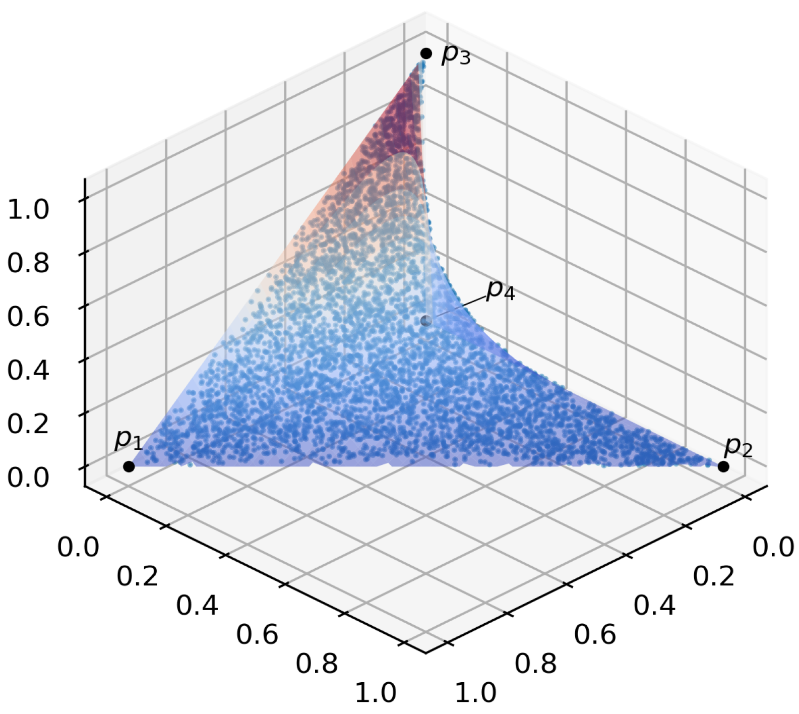
We aim to generate discrete probability distributions with components $(p_1,p_2,p_3,p_4)$ that satisfy the above constraints for an arbitrary input vector. The basic neural network is represented as one softmax layer, and the additional differentiable layer with output satisfying these constraints. The admissible points belong to a surface in the 3-dimensional space, which is shown at Figure 4. The probability simplex extreme points or vertices are denoted as $p_i$.

We define the SDF as follows:

$${\sigma }_{\Omega }=(p_1·(p_1+p_2+p_3-1)+p_2·p_3),$$

(51)

and try to generate points on the surface, i.e., where ${\sigma }_{\Omega }=0$.

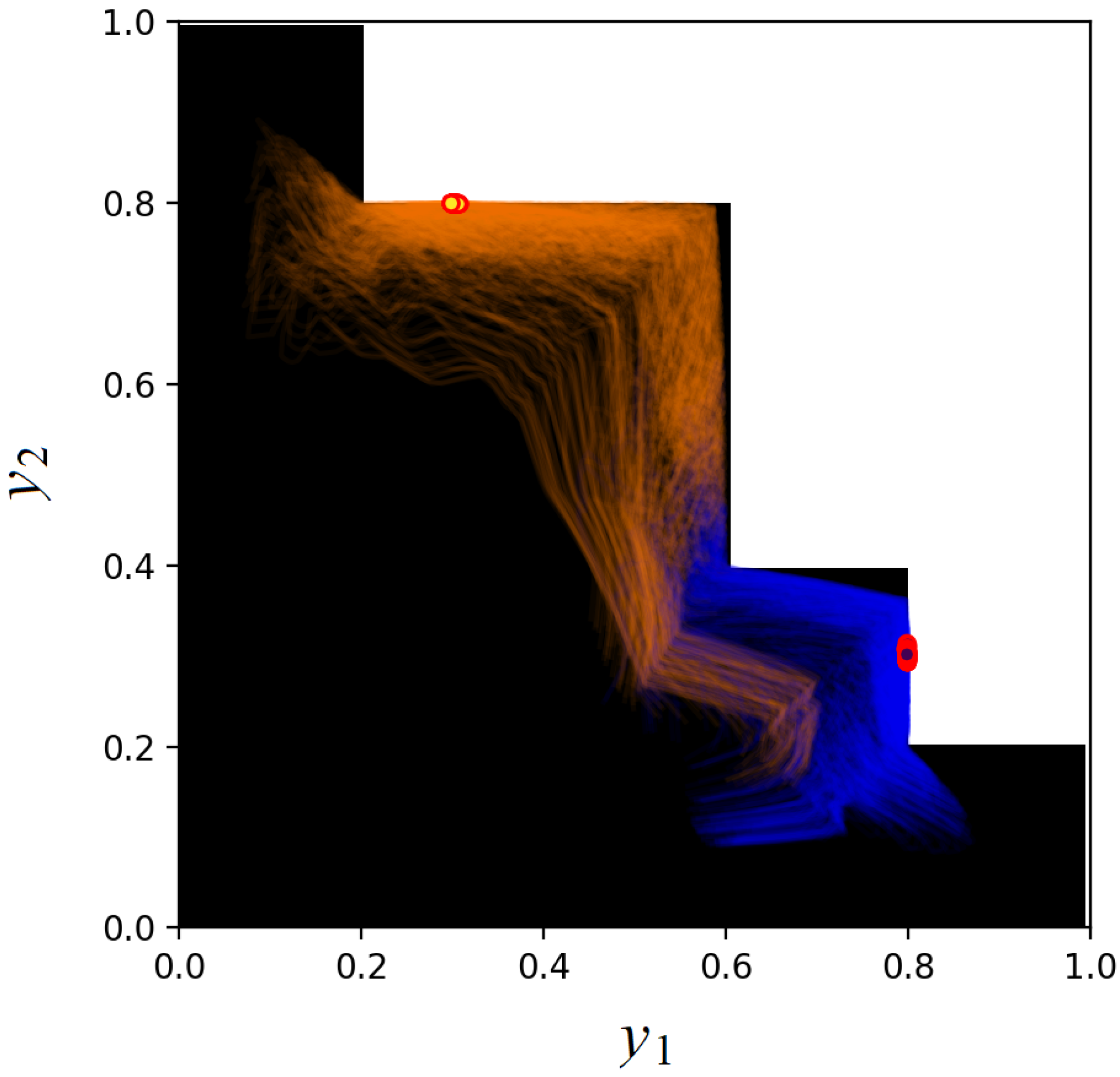
7.2. Personalized Treatment Under Dose Constraints

As an example of the neural network training with the proposed constrained layer, we consider a problem of choosing doses of chemotherapy ($y_1$) and radiation ($y_2$) based on patient feature vector with synthetically generated data [27,28]. In this problem, it is important that no dose ratio is acceptable. The constraints are defined as a union of multiple rectangles, obtained by intersection of axis-parallel hyperplanes, and the admissible set has a ladder-like shape. The patient vector z in the example consists of three features, where only the first feature is significant. Each feature is sampled from the uniform distribution in the interval $[-1,1]$. The neural network takes the patient feature vector z as an input and predicts the dose estimation $\widehat{y}=({\widehat{y}}_1,{\widehat{y}}_2)$, satisfying the constraints. The loss function depending on the input vector z and the estimated dose $\widehat{y}$ is determined as follows:

$$l(z,\widehat{y})=\left\{\begin{array}{cc}{({\widehat{y}}_1-0.3)}^2+{({\widehat{y}}_2-0.9)}^2,\hfill & z_1\ge 0,\hfill \\ |{\widehat{y}}_1-0.9|+{({\widehat{y}}_2-0.3)}^2,\hfill & z_1<0.\hfill \end{array}\right.$$

(52)

The neural network parameters are optimized to minimize the loss over elements of the dataset:

$$\sum _{i=1}^{N}l\left(z^{\left(i\right)},f_{\theta }\left(z^{\left(i\right)}\right)\right).$$

(53)

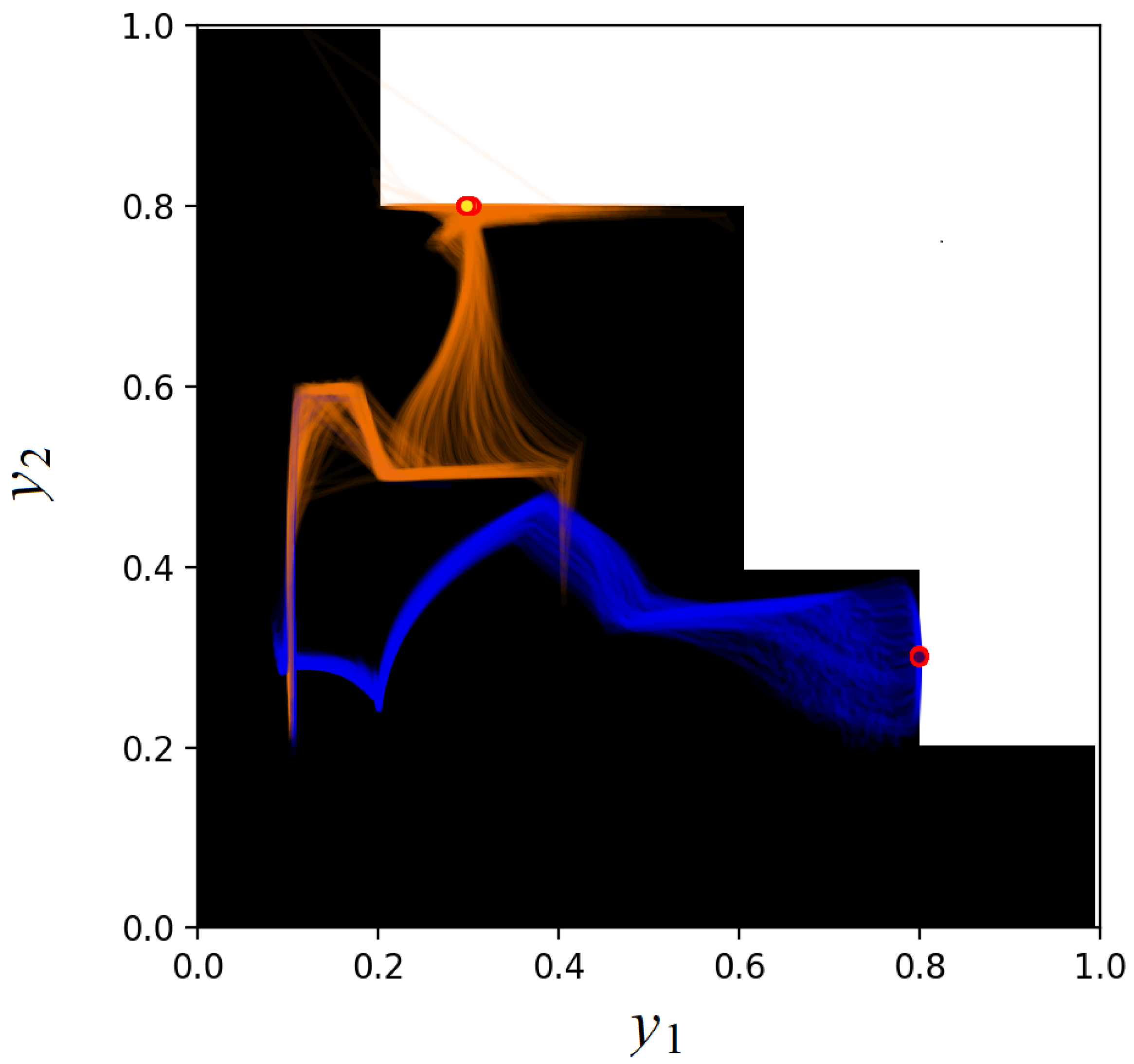
We use the following hyperparameters of the neural network: 3 layers having 8 units with SiLU activations, trained with Adam with the learning rate ${10}^{-4}$, a batch size of 16 for 1000 epochs on the dataset consisting of 500 synthetically generated patient vectors. Also, we limit the number of ray marching iterations to 5. The dataset consists of 500 points. The semi-transparent blue and orange curves in Figure 5 and Figure 6 represent trajectories of estimated doses $f_{\theta }\left(z^{\left(i\right)}\right)$ for every dataset point over training iterations, for negative and positive values of $z_1$, respectively. 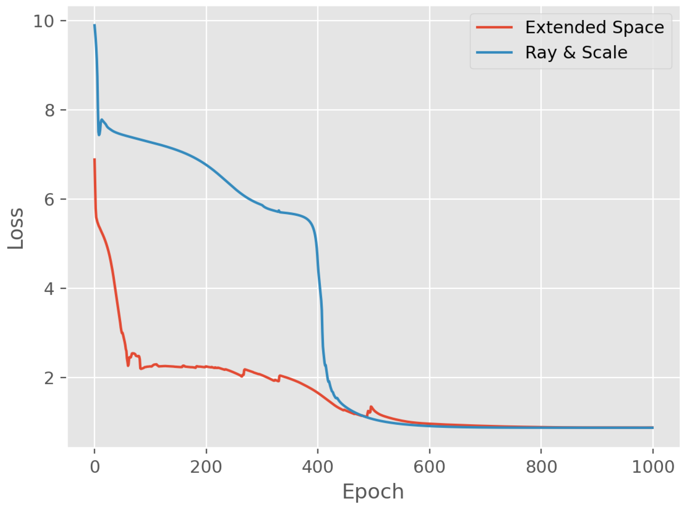Figure 5 illustrates the ray and scale approach, whereas Figure 6 shows results of the extended space approach. The final predictions are shown as blue and orange circles with red boundary. The loss functions are shown in Figure 7. It can be seen from Figure 5 and Figure 6 that trajectories resemble the shape of the admissible set when a separate value is used for determining the point inside the admissible ray segment. This is because the ray direction and the scale are calculated and optimized as separate variables. The extended state approach does not have such a peculiarity. Also, due to different parameterization, trajectories in the extended space approach are much more diverse. Interestingly, both approaches, even with different outputs before training, converge almost identically starting from 500 iteration.

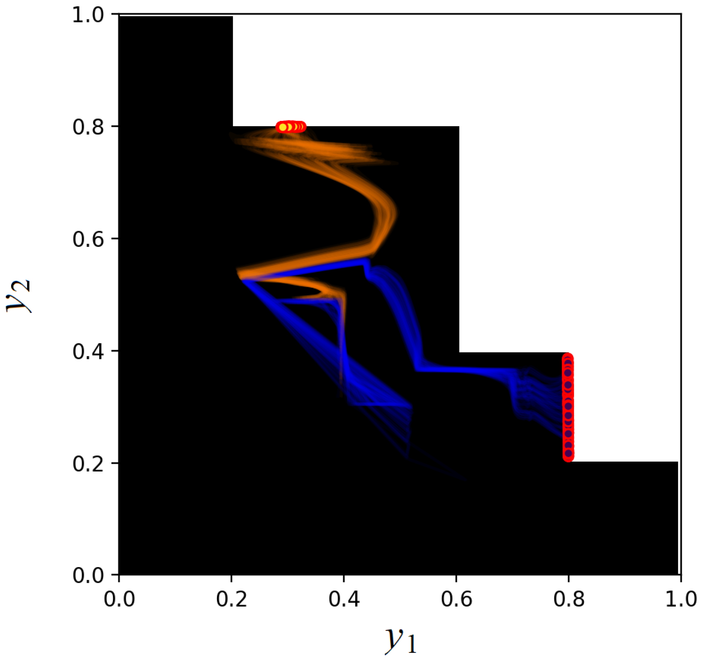
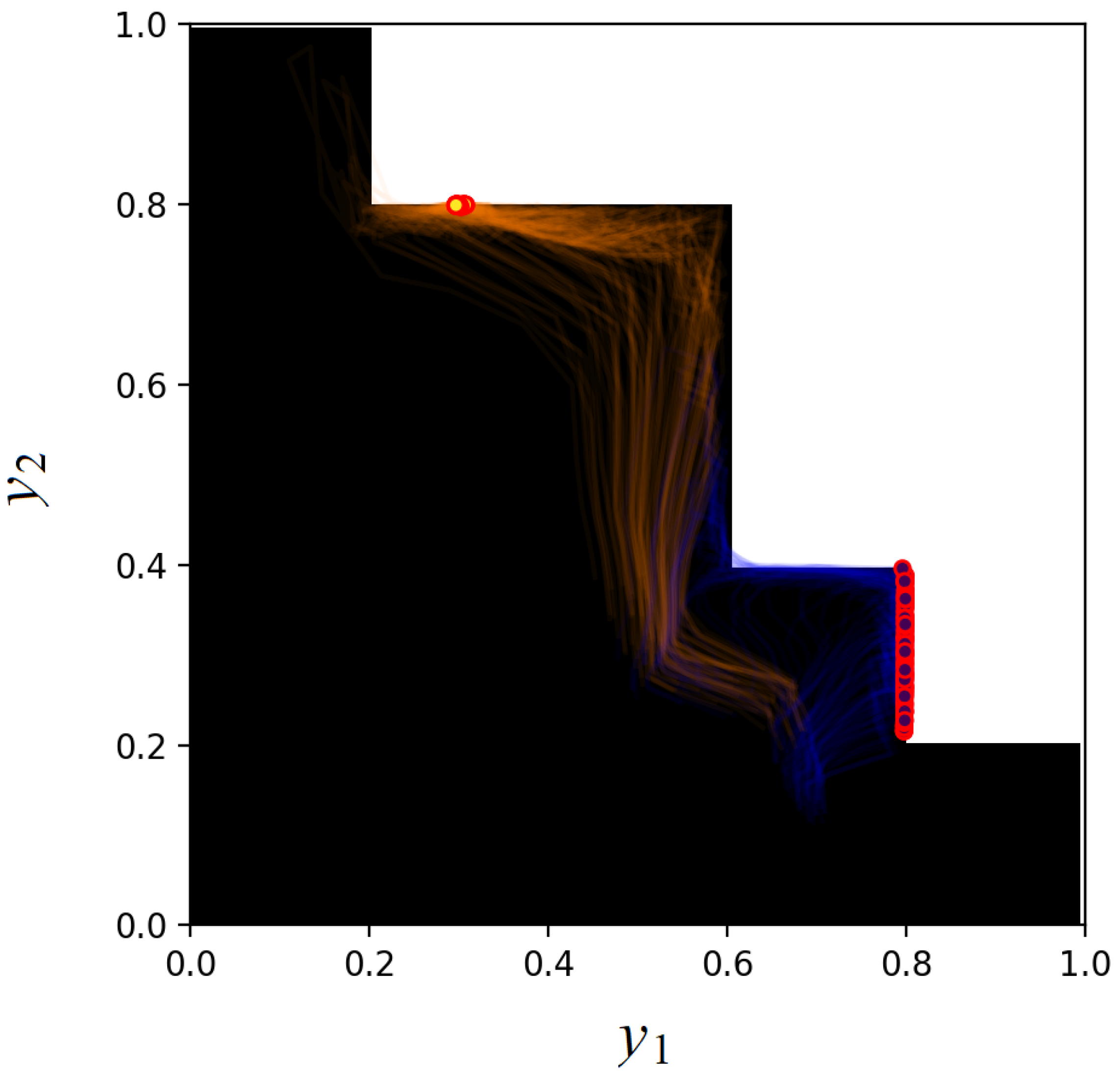
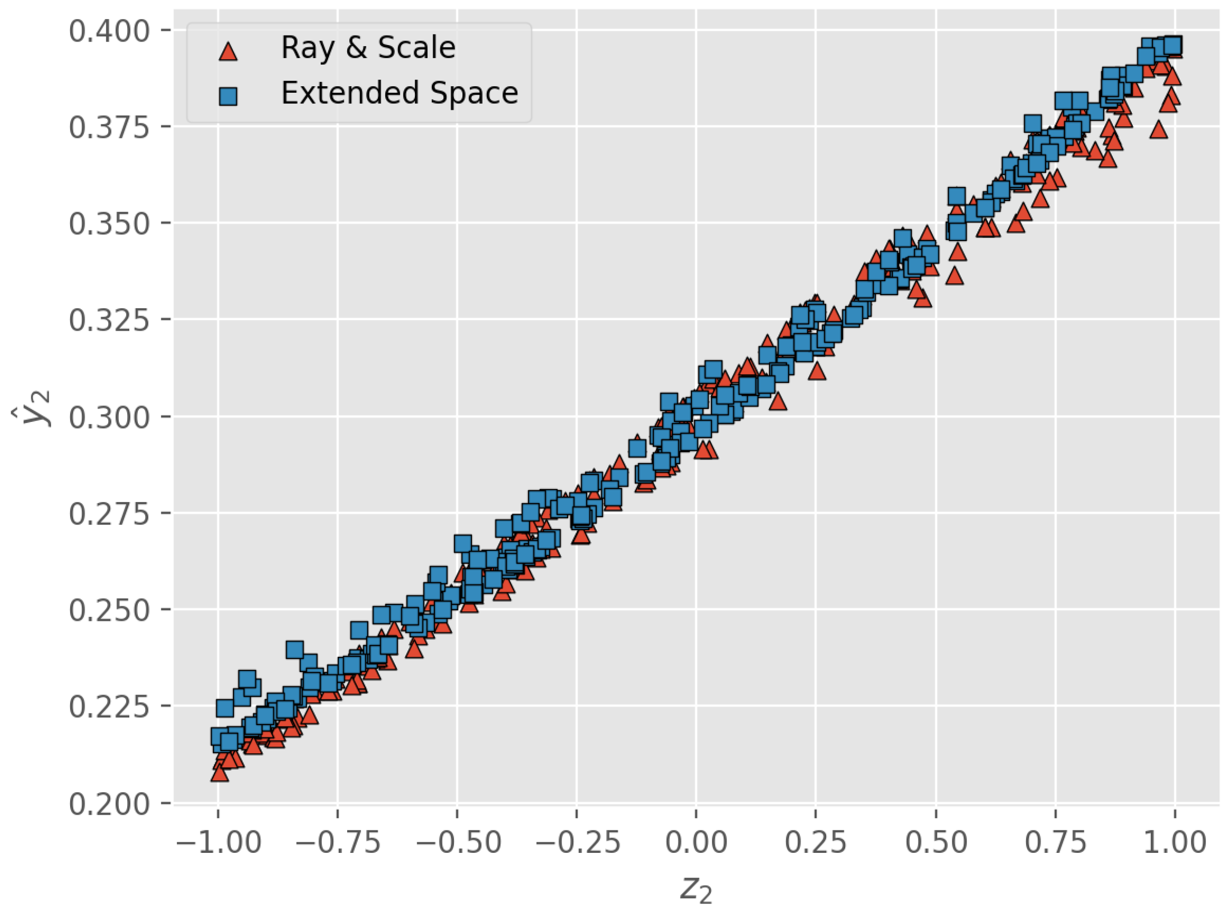
Let us consider the second example of the personalized treatment problem, where the loss function partially depends on the second feature $z_2$ of the input:

$$\tilde{l}(z,\widehat{y})=\left\{\begin{array}{cc}{({\widehat{y}}_1-0.3)}^2+{({\widehat{y}}_2-0.9)}^2,\hfill & z_1\ge 0,\hfill \\ |{\widehat{y}}_1-0.9|+{({\widehat{y}}_2-0.3-0.1·z_2)}^2,\hfill & z_1<0.\hfill \end{array}\right.$$

(54)

It can be seen from the above that the optimal solution in the case $z_1<0$ without constraints is ${\widehat{y}}_1=0.9$, ${\widehat{y}}_2=0.3+0.1·z_2$. Figure 8 and Figure 9 represent the same trajectories of estimated doses $f_{\theta }\left(z^{\left(i\right)}\right)$ by using the ray and scale approach (Figure 8) and the extended space approach (Figure 9). Figure 10 shows how the predicted value ${\widehat{y}}_2$ depends on the second feature $z_2$ of the input for cases of using the ray and scale and the extended space approaches. It is interesting to point out that, in contrast to the previous example, the optimal solution is not concentrated at one point, it is spread out in the interval of ${\widehat{y}}_2\in [0.2,0.4]$. It can be seen from Figure 10 that the neural network has learned the linear dependence on $z_2$ in case of $z_1<0$ correctly (the Pearson correlation coefficient is larger than $0.995$ in both cases), while in the other case $z_1\ge 0$, the learned solutions are concentrated around one point $(0.3,0.8)$.

Trajectories of estimated doses obtained in accordance with the Ray & Scale and the extended space approaches when the loss function partially depends on the second feature $z_2$.

8. Conclusions

A method imposing hard constraints in the form of a star-shaped region on the neural network output values has been presented. It is implemented by adding a layer to the neural network, which generates a parameterized shift of the origin towards a ray. The method can be applied to various problems which require the restriction of the neural network output by certain constraints, for example, constrained optimization problems and physics-informed neural networks.

The main limitation of the proposed method is that $\Omega$ should be star-shaped. Approaches to handle more complex cases is a problem whose solution meets many obstacles. Therefore, this important problem can be regarded as a direction for further research.

Results presented in the paper can be viewed as a general approach to constructing neural networks with the star-shaped constraints imposed on the network output. Specific applications of the approach to certain real problems could significantly simplify it by means of its adaptation to a the problem peculiarities. The implementation of the approach to various real problems forms a set of other interesting directions for further study.