Article

Iterative Optimization RCO: A “Ruler & Compass” Deterministic Method

1
Independent Consultant, 74570 Groisy, France
2
Laboratory of Images Signals and Intelligent Systems (LiSSi), University of Paris-Est Créteil (UPEC), 94000 Créteil, France
Mathematics 2024, 12(23), 3755; https://doi.org/10.3390/math12233755
Submission received: 1 October 2024 / Revised: 23 October 2024 / Accepted: 25 November 2024 / Published: 28 November 2024
(This article belongs to the Section E1: Mathematics and Computer Science)

Abstract

:
We present a basic version of a deterministic iterative optimization algorithm that requires only one parameter and is often capable of finding a good solution after very few evaluations of the fitness function. We demonstrate its principles using a multimodal one-dimensional problem. For such problems, the algorithm could be applied with just a ruler and a compass, which is how it got its name. We also provide classical examples and compare its performance with six well-known stochastic optimizers. These comparisons highlight the strengths and weaknesses of RCO. Since this version does not address potential stagnation, it is best suited for low-dimensional problems (typically no more than ten), where each evaluation of a position in the search space is computationally expensive.
MSC:
90C26; 65K99

1. Introduction

In iterative optimization, and for some problems, the cost of each evaluation can be very high. Additionally, many algorithms are stochastic, meaning they need to be run multiple times. Therefore, a method that requires only one run and may find a good solution after just a few evaluations could be highly beneficial. As mentioned, this approach does not work for every problem, but it is generally worth trying before moving on to a more costly stochastic method.
The only parameter required is the lower bound, which is often reasonably well-known in practice. Furthermore, there is an optional adaptive lower bound, in which case no parameter is needed.
Several definitions of the theoretical a priori difficulty of an optimization problem (minimization here) have been proposed [1]. For example, one can consider the number of local minima and the relative size of the subspace of acceptable solutions. If this number is high and the size small, then any iterative algorithm functioning as a black box would require numerous samples of positions in the search space and, therefore, many evaluations of positions.
Consider the multimodal one-dimensional function whose landscape is shown in Figure 1, where the minimum is 0.999507 at position 2.412616. Although it is one-dimensional, its theoretical difficulty is high because it has many local minima.
For the algorithms tested below, we say that a solution is acceptable if its value is less than 0.9997.
For stochastic algorithms, we estimate the probability of success by running them a thousand times.
Table 1 then shows that, for these, many evaluations are needed to have a good chance of finding a satisfactory solution and, therefore, the actual difficulty (large number of evaluations) is in good agreement with the theoretical difficulty.
However, it is possible to define a deterministic (in the non-stochastic sense) algorithm, for which this agreement is challenged. On this problem, the Ruler & Compass Optimizer (RCO) is extremely efficient (see Figure 2). More generally, it is also effective on other supposedly difficult problems. Furthermore, conversely, it can be highly ineffective on problems that are supposed to be easy.
Thus, the mere existence of such an algorithm largely calls into question the relevance of classical difficulty estimates, which will have to be revised, at least by specifying their field of application in the space of optimizers.
Informally, the No Free Lunch Theorem [2] allows us to say that there is no such thing as an efficient optimizer for all problems. If “efficient” is to be interpreted as “finding a solution without too much difficulty”, then what RCO suggests is a dual proposition: there is no a priori measure of difficulty valid for all optimizers.
Analyzing this conjecture is not the purpose of this study. In what follows, we will look at the detailed operation of RCO and show on other examples how its behavior is atypical. This will allow us to sketch a typology of problems for which it is interesting to use it.
Table 1. On the problem in Figure 1, metaheuristics, as expected, sometimes struggle to find an acceptable solution with a high probability, estimated over 1000 executions. Since RCO is deterministic, only one run is required.
AlgorithmStochasticEvaluations/RunSuccess Rate
CMA-ES [3]yes10,0000.12
DE [4]yes10,0000.73
ACO [5]yes4100.80
40100.94
Jaya [6]yes10000.985
SPSO [7]yes1800
1901
GA-MPC [8]yes800
901
RCOno201

2. RCO Principle

On our Test landscape, RCO finds a definite acceptable solution after 20 evaluations (see Figure 2).
However, to detail the iterative construction, it is better to consider a simpler example, defined by:
f x = x 3 2 f o r x 0 , 10
where its minimum is obviously 0 on x = 3 .
For this basic version, a user-defined parameter is needed: a fixed lower bound. Note that in practice, we often know one. Moreover, RCO is in fact able to use an adaptive one, automatically estimated during the process (see Appendix A.5), but the figures are then more difficult to understand.
Here, we set this lower bound to −5, to more clearly see what happens, although −0.1 would be sufficient.
Table 2, Table 3, Table 4, Table 5 and Table 6 illustrate the process. Of course, in higher dimension D the lines become (hyper-)planes but the method is the same. At each time step, we consider D planes defined by D + 1 points and their intersection point (it may happen that there is more than one unique intersection point; if so, we consider we are in the case 1) with the lower bound plane. There are two cases:
  • If its position lies outside the search space (possibly at infinity), then the new position is determined by a barycenter of the 2 D previous positions. For the calculation of the barycenter, the weight of each position is inversely proportional to the value of the function at that position. See the detail in Appendix A.2.
  • If its position is within the search space, then it is kept as the new position.
Then, in the list of positions, the first one is removed and the new one is added.

3. Examples

The definitions of the problems are given in Appendix A.7. Some of them have been shifted in order to be not too easy.

3.1. Six Hump Camel Back (Appendix A.7)

The dimension of the problem is two, so the landscape has four corners. The search space is 2 , 2 × 1 , 1 .
The minimum is −1.031628453489877. A definite lower bound is −1.1. Table 7 shows the results for increasing number of evaluations and Figure 3 the construction for 14 evaluations.

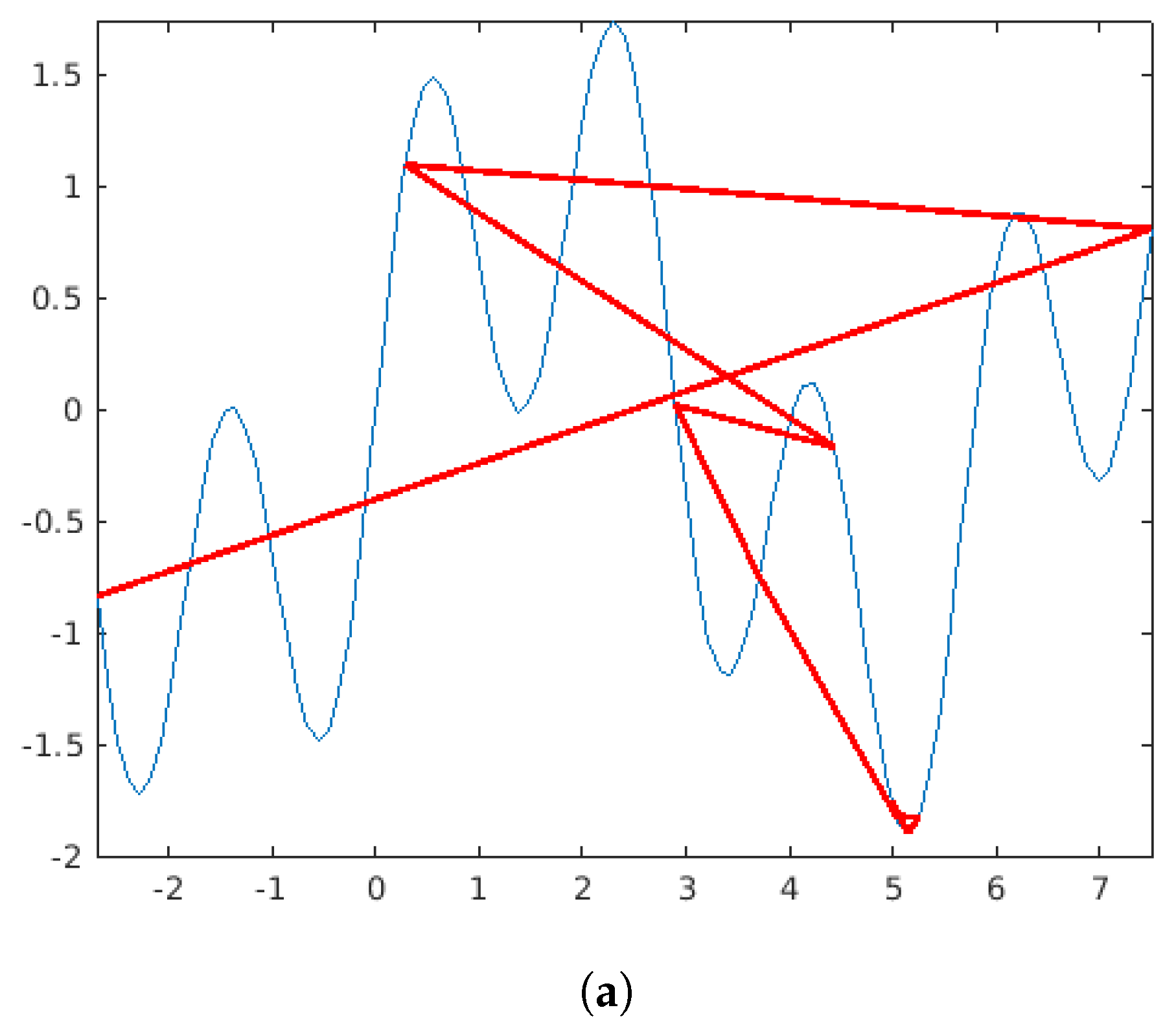
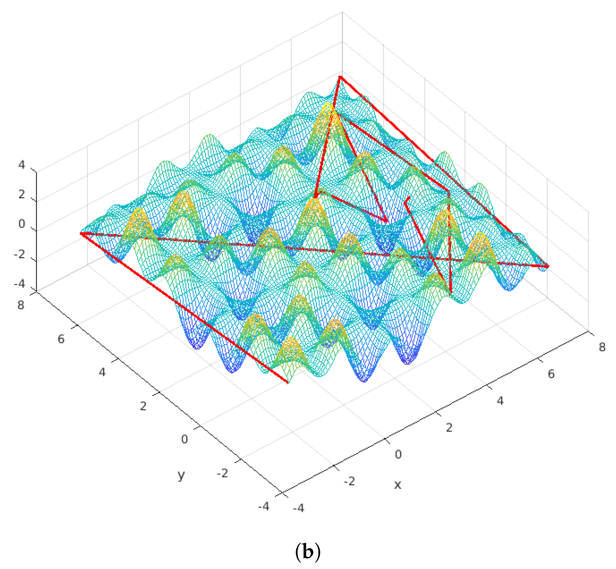
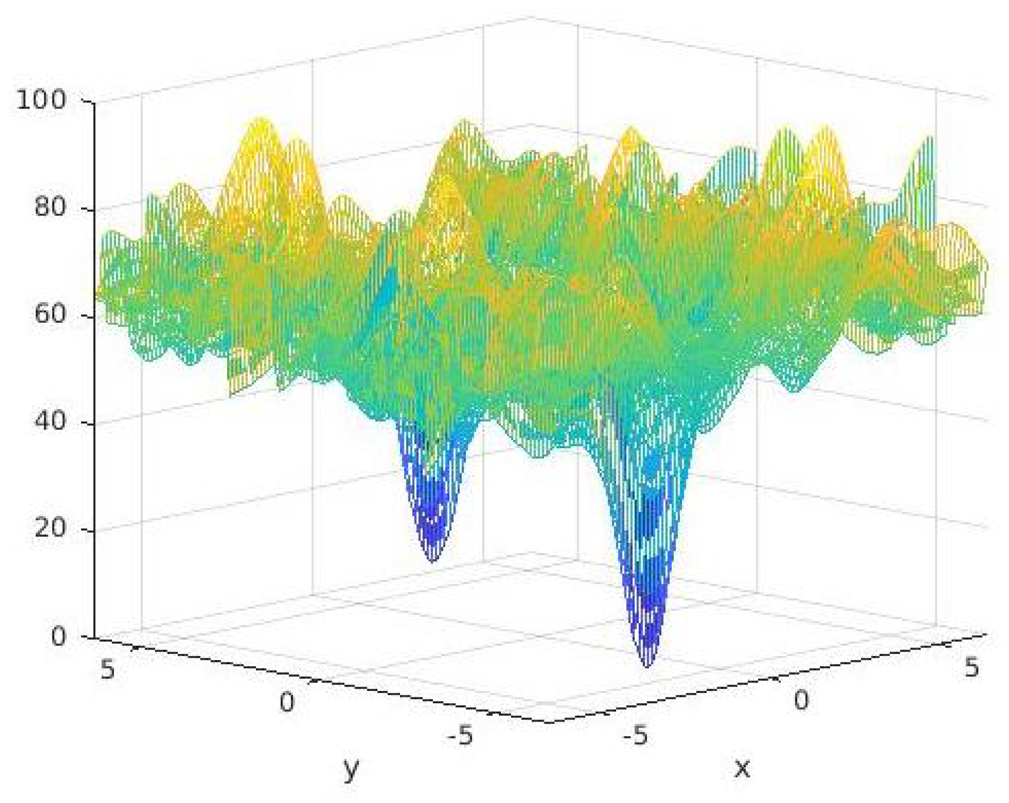
3.2. Shifted Rastrigin
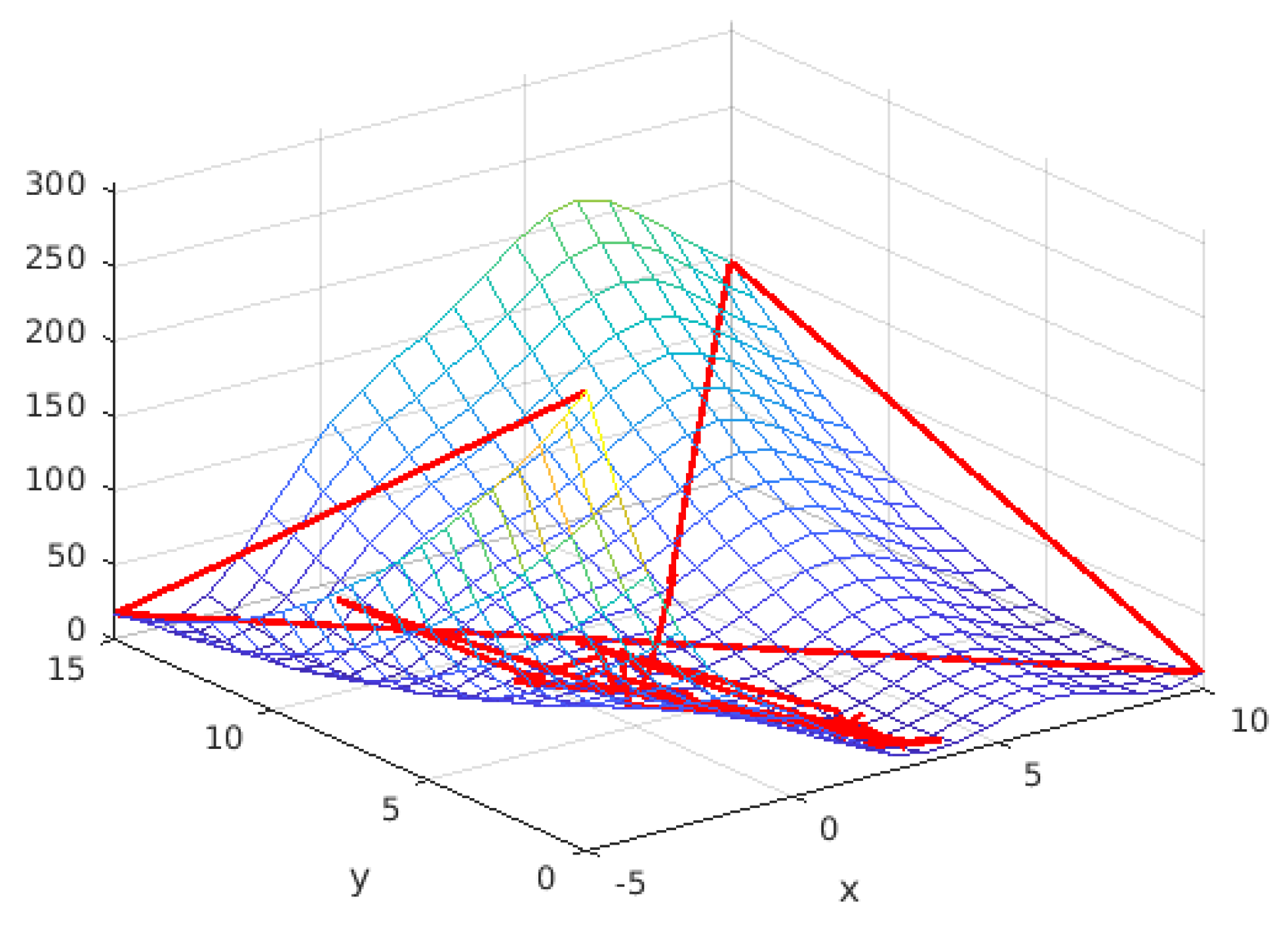
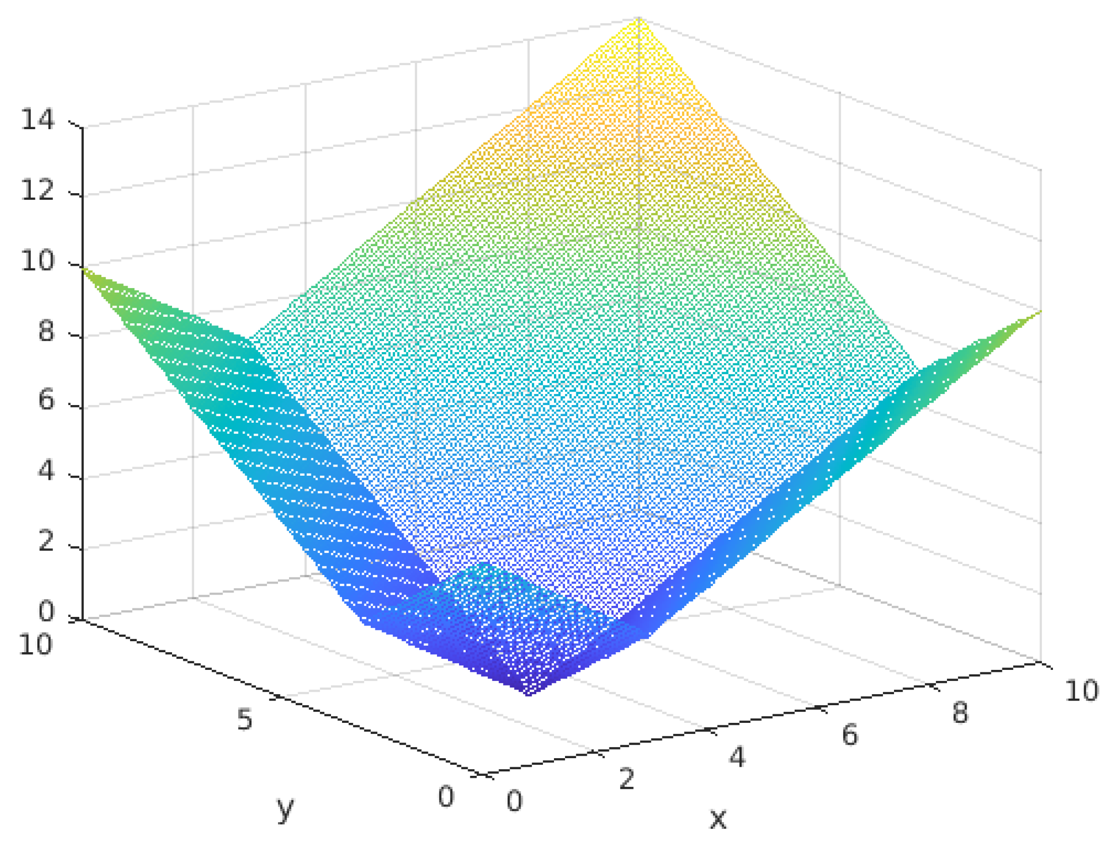
(See Appendix A.7 for details).
The minimum is zero, so a definite lower bound is −0.1. Table 8 shows the results for different dimensions and different numbers of evaluations and Figure 4 the constructions for 1D and 2D landscapes after 12 and 14 evaluations, respectively.

3.3. Rosenbrock

(See Appendix A.7 for details).
The minimum is zero, so a definite lower bound is −0.1. Table 9 shows the results for dimensions two to five with an increasing number of evaluations.

3.4. Pressure Vessel

(See Appendix A.7 for details).
There are four values to find, where the two first ones are discrete. The minimum value is 6059.714335048436, as proved in [9].
The lower bound used here is 6000. Table 10 show the results for an increasing number of evaluations. Due to the discrete variables, the algorithm encounters difficulties in converging.

3.5. Gear Train

(See Appendix A.7 for details).
There are four values to find, all discrete. The minimum is 2.700857 × 10 12 .
Here, the lower bound is simply set to 0. As we can see in Table 11, the algorithm quickly proposes a solution that is far from optimal, and then stagnates without further improvement.

4. Comparison

Let us compare RCO with a slightly improved version of Standard PSO (SPSO-Dicho on my technical website [10]. To favor PSO, I have selected the best run out of five. The results are presented in Table 12. Also, refer to Figure 5 for Shifted Griewank, where the two methods appear to be equivalent, particularly for dimensions 1 to 5 and the number of evaluations, respectively set to 100, 200, 5000, 10,000, and 20,000.
In lower dimensions (less than 10), RCO performs better and sometimes significantly so. However, for higher dimensions, RCO stagnates while PSO continues to find better solutions, as evidenced by Shifted Rastrigin and Rosenbrock.

5. Complexities

To assess an algorithm, it is common practice to conduct a theoretical analysis of both its space complexity and time complexity. However, as explained in [11], this approach is not always appropriate, and a more reliable method is to estimate the actual memory usage and computational time.
In this context, there are two possible scenarios at each time step:
  • Solving a linear system of D equations to determine a new position with D coordinates. The required space is D 2 + D , with a time complexity of O ( D 3 ) .
  • Computing a linear combination of 2 D positions, each with D coordinates. The required space is O ( D × 2 D ) , and the number of multiplications is O ( 2 D ) .
However, such a classical reasoning does not correspond to the behavior of the algorithm in practice. The point is that the second situation usually does not occur very often except at the end of the process. Moreover, it depends on the landscape of the problem and also on the “budget” (the maximum acceptable number of evaluations).
Let us consider, for example, the computing time per evaluation for two problems: Planes and Shifted Rastrigin. We have already seen the Shifted Rastrigin and Planes is defined by:
f x = d = 1 D x d 3
Figure 6 depicts its landscape in two dimensions.
As we can see in Table 13, the real computing time indeed grows exponentially, but more like 1.35 D than 2 D .

6. A Problem That RCO Cannot Solve

In some instances, even when problems are continuous and of low dimension, RCO does not perform well. For instance, let us examine the Frequency Modulated Sound Waves from the CEC 2011 competition benchmark [12]. The search space is 6.4 ,   6.35 6 and the minimum value is zero. Despite 50,064 evaluations, the best final value achieved is 24.07. This is primarily due to a considerable number of intersection positions (21,238) lying outside the search space, rendering them unacceptable.
It is worth noting that in such cases, expanding the search space might provide some benefit if feasible. For example, if the search space is expanded to 500 ,   500 6 , there are 17,322 unacceptable intersections, resulting in a final best value of 17.42. However, many classical stochastic algorithms tend to discover significantly better solutions. This is because stochasticity can effectively navigate a highly chaotic landscape, as is the one of FMSW (see Figure 7). For example, the slightly improved PSO already mentioned needs just two runs to find 2.218602 × 10 27 .

7. Conclusions and Future Works

Even in low dimensions, evaluating the objective function can sometimes be very costly. In such cases, RCO may be beneficial as it may propose a good solution after only a few evaluations. However, there are some disadvantages:
  • It requires a reasonably good lower bound. That said, compared to most other methods, this is the only user-defined parameter. In practice, for real-world problems, such a bound is often known. Moreover RCO is able to automatically define an adaptive lower bound (see Appendix A.5).
  • It performs poorly on some problems, even in low dimensions, when the landscape is highly chaotic.
  • It does not perform well on discrete problems, particularly when all variables are discrete. However, it still appears to be usable when only some of the variables are discrete.
  • Its computation time per iteration increases exponentially with the dimension of the search space. Although it does not grow as quickly as theoretically predicted, in practice, it can still be challenging to use on a laptop for high-dimensional problems.
  • As with many initial presentations of iterative optimization algorithms, such as Genetic Algorithm [13], Ant Colony Optimization [14], Particle Swarm Optimization [15], and Differential Evolution [16], among others, a formal convergence analysis has not yet been provided. Specifically, while it is clear that there is no explosion effect, as seen in the original PSO version [17], it would be beneficial to more precisely identify in which cases stagnation occurs and how it can be avoided. There is, in fact, an experimental RCO version that attempts to address the issue of stagnation, though it is not particularly convincing. For instance, in the case of the 10D Rosenbrock function (see Table 12), it finds a value of 2.3 instead of 8.996, which is still significantly worse than PSO ( 5.19 × 10 8 ).

Funding

This research received no external funding.

Data Availability Statement

The original contributions presented in the study are included in the article, further inquiries can be directed to the author.

Conflicts of Interest

The author declares no conflicts of interest.

Appendix A

Appendix A.1. A Bit of Geometry

To perform the “Ruler & Compass” construction in one dimension, as depicted in  Figure 3, it is necessary to define two segments, denoted as a and b, such that a/b = A/B. This method, dating back over 2600 years to Thales of Miletus, may have slipped from your memory over time; thus, Figure A1 illustrates the procedure.
Figure A1. Ruler & Compass method to define proportional segments.
Mathematics 12 03755 g0a1

Appendix A.2. Barycenter

More generally we define the barycenter x N e w of the 2 D current positions x thanks to the values of the function f on these positions. See below the Octave/Matlab code of this calculation.
  
% Barycenter
minf=min(f);
if minf>=0 w=sum(f)-f; else w=sum(f-minf)-(f-minf); end
if w>0  xNew=sum(w’.*x)/sum(w);
else xNew=mean(x); end % Particular case, w may be null
  
Note: Of course, other formulas are possible—particularly those that use the differences between the f-values and the lower bound—but this one seems to produce good results.

Appendix A.3. Number of Minima

In black box optimization of a non-discrete function, it is theoretically impossible to know the number of (local) minima, because the set of positions contains an infinite number of points. On a digital computer, it is theoretically possible by exhaustive search, because with an ε -machine, the number of positions is finite. However, this number will still be huge (typically 2 53 D for a definition space of dimension D).
So, we have to make a comprise: an exhaustive search on a grid whose spacing is not too large (which may generate many fake minima) and not too small (too much computing time, numerical instability).
Then the following algorithm for a function f may be useful:
  
Define a grid with N positions along each dimension
For each position x evaluate  f x , and also the values  f i = f x i  of the neighbors  x i  (usually  2 D  except on the frontier).
If  f x < f i  for all i, then assume that x is a (local) minimum.
  
This algorithm requires about 2 N + 1 evaluations, but does not need a large memory size. We could evaluate just once each position and save the result, but then the memory size would be big. Furthermore, for each position, we would have to find if it has been already evaluated.
When two neighbors on the grid have the same value, the algorithm may assume they are both “minima”, as we can see in Figure A2.
By applying this algorithm, we find that the landscape of sinCos15 has 28 minima in dimension one (and 818 in dimension two), including just one global minimum (see Figure 1). Six Hump Camel Back has six minima, including two global ones. Furthermore, naturally, Parabola is unimodal. For the Frequency-modulated Sound Waves, we find that there are at least 99,325 minima. Further refinement would be too time consuming.
Figure A2. Looking for minima, the algorithm may find fake minima when two neighbors (here 2 and 4) on the grid have the same value.
Mathematics 12 03755 g0a2

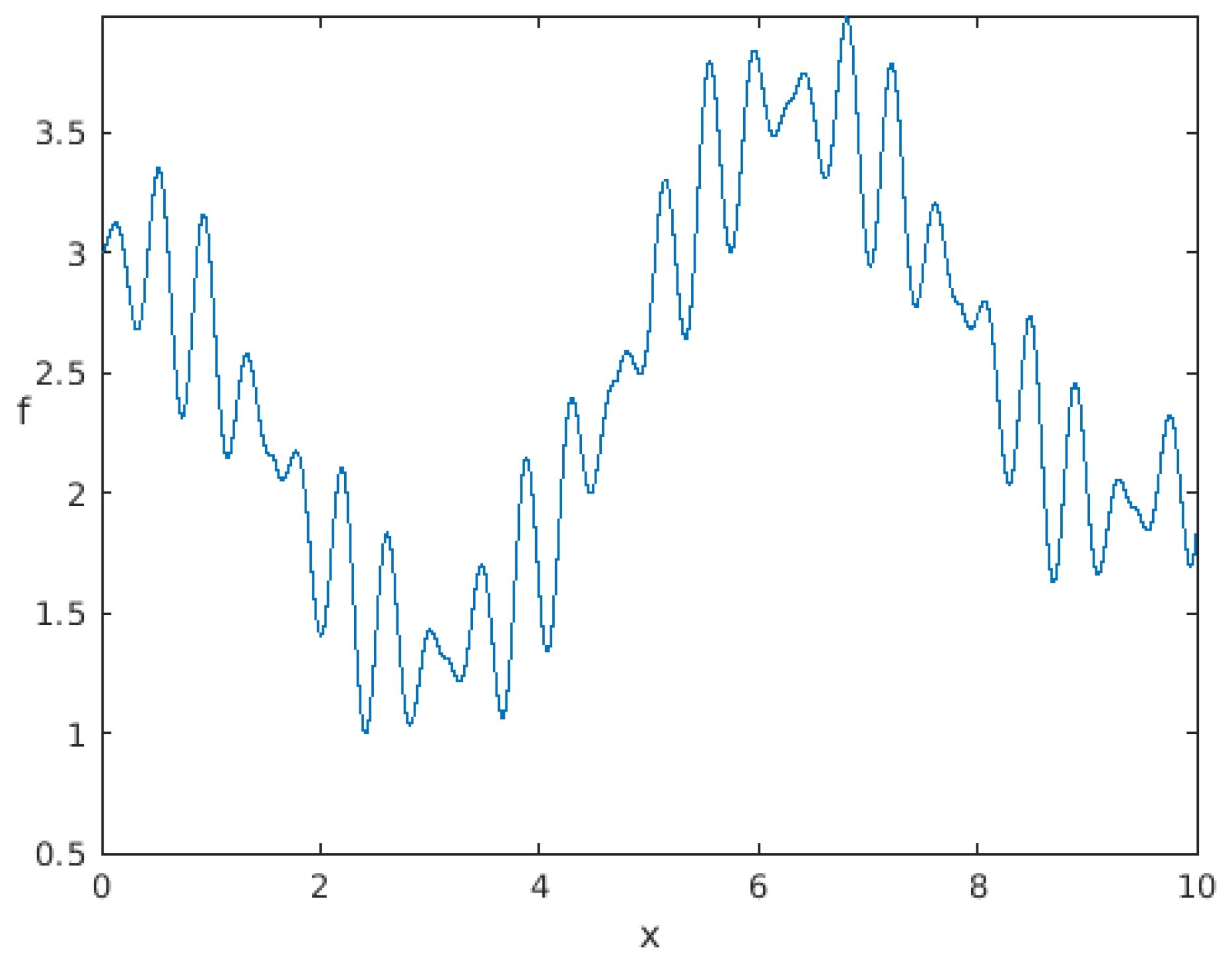
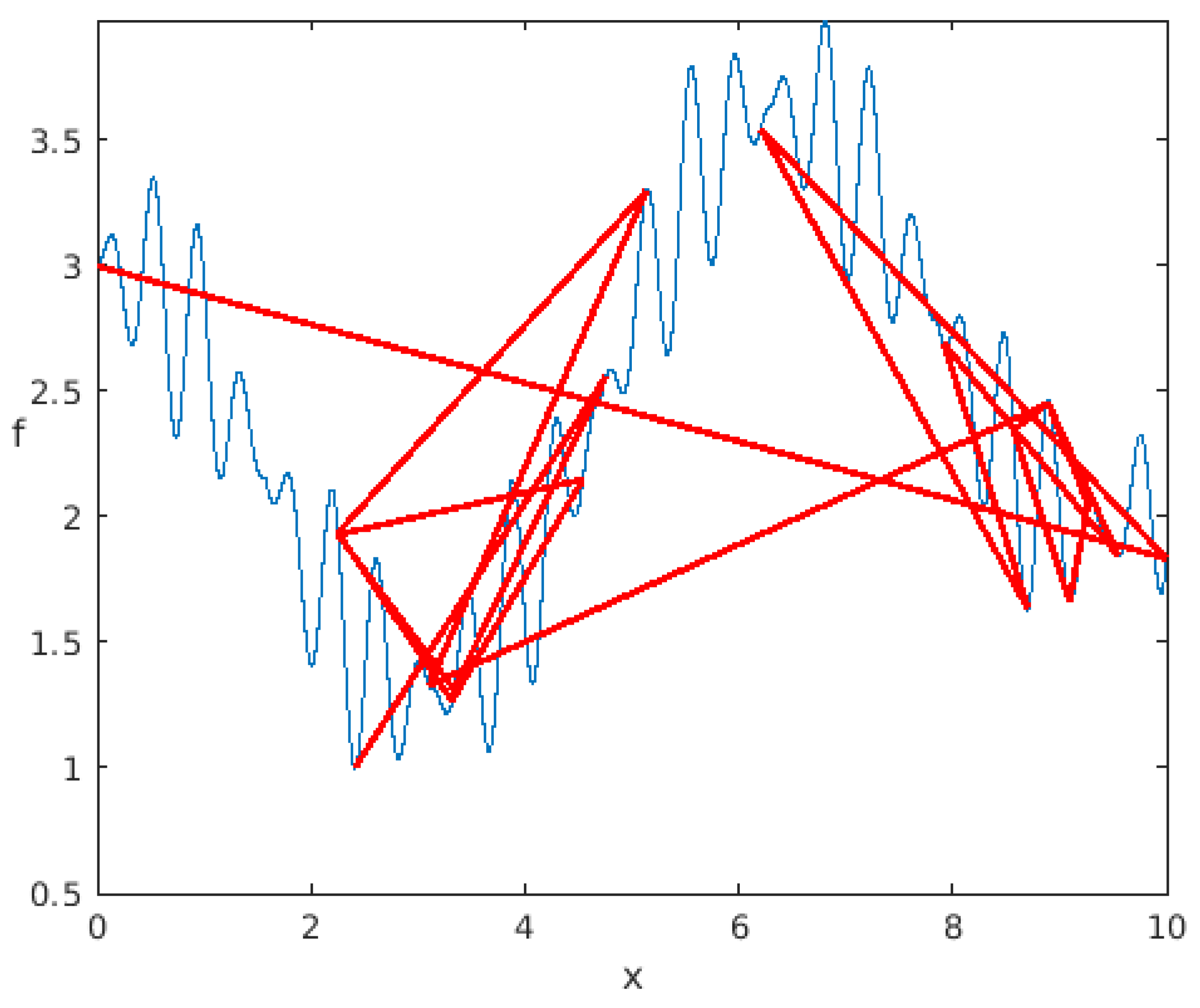
Appendix A.4. Difficulty Measures

Detailed descriptions, examples, and references can be found in [1]. As explained in this Reference, the δ ¬ N i s B measure is interesting, for it implicitly takes into account not only the number of local minima but also the sizes of their attraction basins. Using a tolerance threshold is usually less discriminant and the normalized roughness is too rudimentary.
Table A1. Difficulty measures in [0, 1]. The ones of Parabola Six Hump Camel Back are given for comparison. The tolerance thresholds are relative to the global minimum value. For sinCos15, it corresponds to a value at most equal to 0.9997, as used in the Introduction.
sinCos15ParabolaSix Hump
Camel Back
Frequency Modulated
Sound Waves
Normalized roughness0.964300.3333>0.9999
Tolerance threshold 1.93 × 10 4 0.99960.99720.999971.0
δ ¬ N i s B 0.47060.07110.62580.5263
As we can see, when considering the sizes of the attraction basins, the difficulty of FMSW is estimated to be less than that of Six Hump Camel Back. This is because, although there are many local minima, each basin is very small. Therefore, many stochastic algorithms can easily escape these minima.

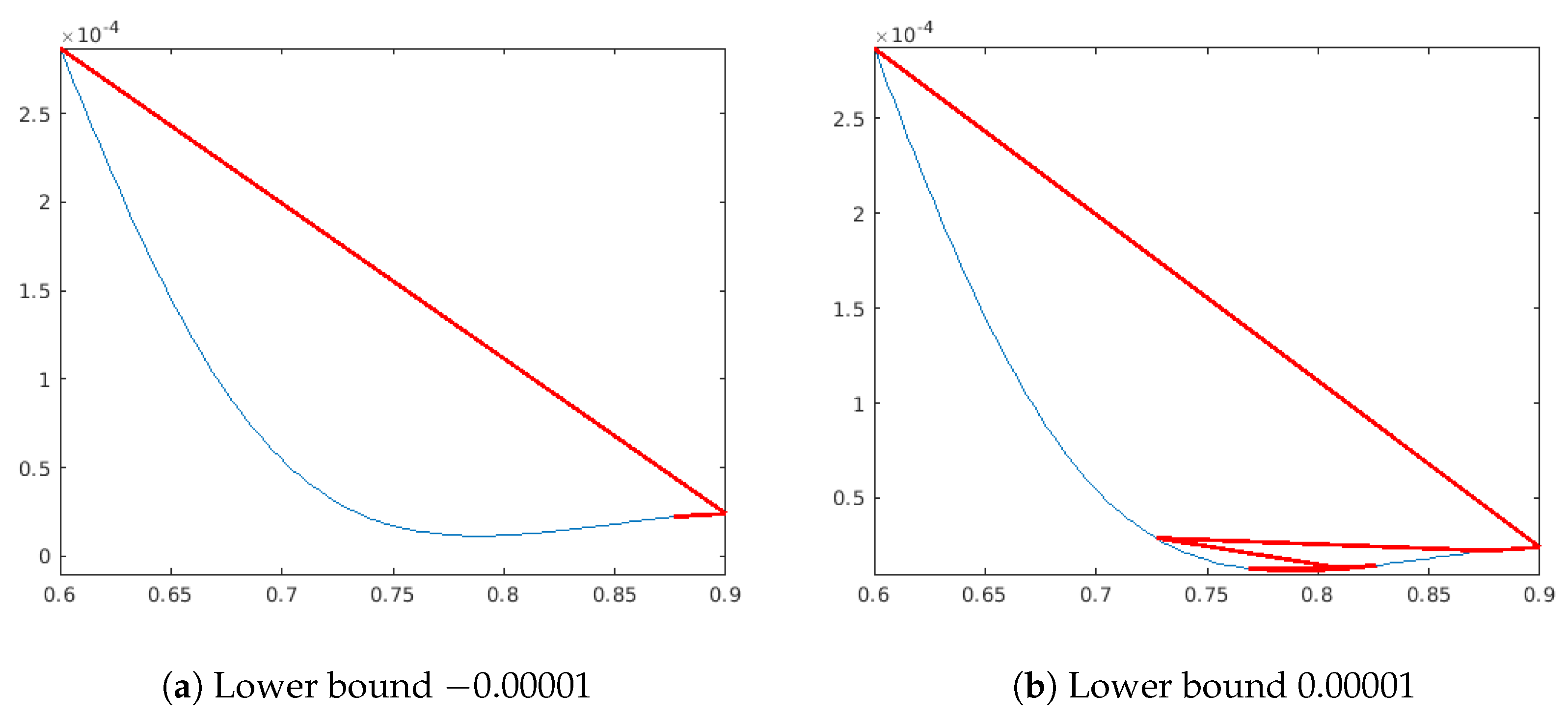
Appendix A.5. About the Lower Bound

As mentioned, the basic RCO needs a user-defined lower bound. Therefore, it is interesting to understand the algorithm’s sensitivity to this parameter. As depicted in Figure A3, we observe that efficiency is indeed sensitive to changes in the lower bound. Though the sensitivity is not extreme, it could still be beneficial to experiment with various values. It is worth noting that setting the lower bound to the exact minimum value, if known, may not be the optimal choice.
Figure A3. Efficiency is somewhat sensitive to the user-defined lower bound, but not excessively so.
Mathematics 12 03755 g0a3
A clear example of sensitivity can be observed when attempting to solve the optimal control problem of the Bifunctional Catalyst Blend in the CEC 2011 competition [12].
As depicted in Figure A4, even a slight modification to the lower bound leads to significantly different behavior due to the very small slope. Conversely, due to the same reason, a position far from the optimal one already exhibits a value close to the minimum.
Figure A4. CEC 2011 Bifunctional Catalyst Blend optimal control problem. Twelve evaluations.
Mathematics 12 03755 g0a4
If you are unsure about the lower bound, you can utilize an adaptive one. This is evaluated as follows after initialization and at each iteration:
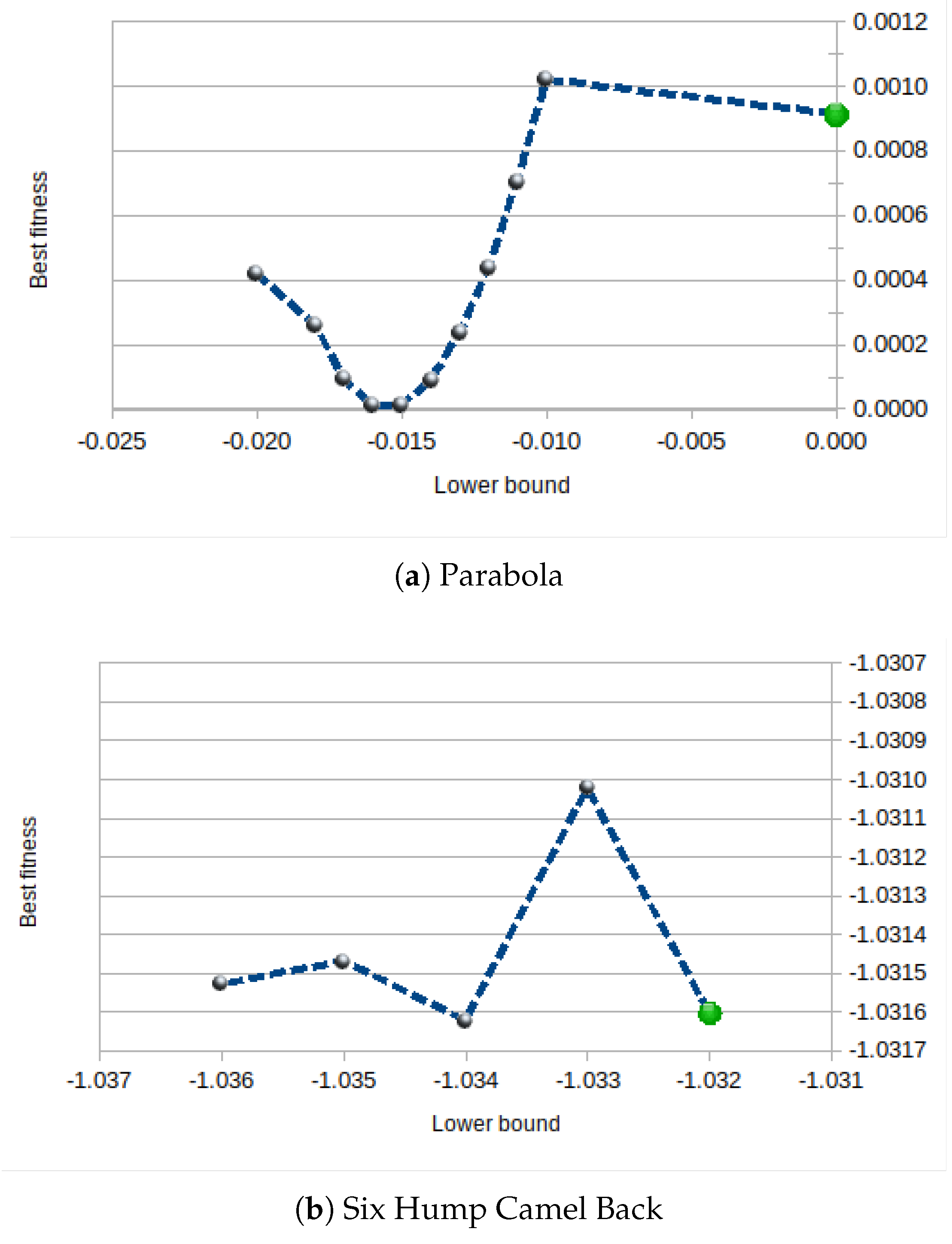
  • if min_f>0 lower_bound=min_f*coeff; else lower_bound=min_f*(2-coeff);
where min_fis the minimum function value found so far and coeff a user-defined parameter in 0 ,   1 .
It appears that the results can occasionally be quite satisfactory, as evidenced by Table A2. Thus, it may be worthwhile to try different methods: user-defined and adaptive ones.
Table A2. Adaptive lower bound may improve the efficiency, or decrease it. The better values are highlighted in bold.
DimensionEvaluationsLower
Bound
Non
Adaptive
Adaptive
Coeff. 0.5
Adaptive
Coeff. 0.1
Six Hump
Camel Back
2104−1.1−1.031473−1.03157−0.947
Shifted Rastrigin31508−0.10.0025480.06729 3.27 × 10 5
450,016−0.10.00173 1.78 × 10 15 0
Rosenbrock31508−0.10.0010.18660.238
410,016−0.10.003756 7.52 × 10 22 8.94 × 10 24
Pressure Vessel46076600065926955 1.29 × 10 5
Gear Train417530 6.65 × 10 9 1.38 × 10 6 6.60 × 10 10

Appendix A.6. More Examples

For amusement, here are a few 1D and 2D figures illustrating how rapidly the algorithm approaches the solution, thanks to steps defined purely by geometry. Initially, they are quite large and gradually diminish in size as they approach the solution’s position.
Figure A5. Multiparaboloid. Fourteen evaluations, final value 0.38 (real minimum 0).
Mathematics 12 03755 g0a5
Figure A6. Branin. Forty-four evaluations, final value 0.3988 (real minimum 0.397887).
Mathematics 12 03755 g0a6
Figure A7. Combination of sinus. (a) Twelve evaluations, final value −1.899584 (real minimum −1.8996). (b) Sixteen evaluations, final value −1.732.
Mathematics 12 03755 g0a7aMathematics 12 03755 g0a7b
Figure A8. Shifted Griewank. Fourteen evaluations, final value 0.34 (real minimum 0).
Mathematics 12 03755 g0a8

Appendix A.7. Problem Definitions

NameDefinitionSearch SpaceMinimum
sinCos15 f = 2 + d = 1 D ( cos x d +
sin x d cos x d sin 15 x d + x d / 10 )
0 ,   10 D 0.999507 for D = 1
Six Hump
Camel Back
4 2.1 x 1 2 + x 1 4 / 3 x 1 2
+ x 1 x 2 + 4 x 2 2 1 x 2 2
2 ,   1 2 —1.031628453489877
Shifted Rastrigin u d = x d 10 d / D + 1 f = 10 D + d = 1 D u d 2 10 cos 2 π u d 10 ,   10 D 0
Rosenbrock f = d = 1 D 1 100 x d + 1 x d 2 2 + 1 x d + 1 2 100 ,   100 D 0
Pressure Vessel 0.0193 x 3 x 1 0 0.00954 x 3 x 2 0 1,296,000 π x 3 2 x 4 + 4 x 3 / 3 0 f = 0.6224 x 1 x 3 x 4 + 1.7781 x 2 x 3 2 + x 1 2 3.1661 x 4 + 19.84 x 3 q = 0.0625 q , 2 q , , 99 2 × 10 ,   200 2 6059.714335048436
Gear Train f = 1.0 / 6.931 x 1 x 2 / x 3 x 4 2 12 , 60 4 2.700857 × 10 12
Frequency
Modulated
Sound Waves
θ = π / 50 y t = t = 1 100 x 1 sin x 2 t θ + x 3 sin x 4 t ϑ + x 5 sin x 6 t θ y 0 = t = 1 100 sin 5 t θ 1.5 sin 4.8 t ϑ + 2 sin 4.9 t θ f = y t y 0 2 6.4 ,   6.35 6 0

References

  1. Clerc, M. Iterative Optimizers—Difficulty Measures and Benchmarks; Wiley: Hoboken, NJ, USA, 2019. [Google Scholar]
  2. Wolpert, D.H.; Macready, W.G. No Free Lunch Theorems for Optimization. IEEE Trans. Evol. Comput. 1997, 1, 67–82. [Google Scholar] [CrossRef]
  3. Hansen, N. The CMA Evolution Strategy: A Tutorial. arXiv 2023, arXiv:1604.00772. [Google Scholar] [CrossRef]
  4. Lampinen, J.; Storn, R. Differential Evolution. In New Optimization Techniques in Engineering; Springer: Berlin/Heidelberg, Germany, 2004; pp. 124–166. [Google Scholar]
  5. Dorigo, M.; Birattari, M.; Stutzle, T. Ant Colony Optimization. IEEE Comput. Intell. Mag. 2006, 1, 28–39. [Google Scholar] [CrossRef]
  6. Da Silva, L.S.A.; Lúcio, Y.L.S.; Coelho, L.d.S.; Mariani, V.C.; Rao, R.V. A comprehensive review on Jaya optimization algorithm. Artif. Intell. Rev. 2023, 56, 4329–4361. [Google Scholar] [CrossRef]
  7. PSC. Particle Swarm Central. Available online: http://particleswarm.info (accessed on 1 November 2024).
  8. Elsayed, S.M.; Sarker, R.A.; Essam, D.L. GA with a New Multi-Parent Crossover for Solving IEEE-CEC2011 Competition Problems. In Proceedings of the 2011 IEEE Congress of Evolutionary Computation (CEC), New Orleans, LA, USA, 5–8 June 2011. [Google Scholar]
  9. Yang, X.S.; Huyck, C.; Karamanoglu, M.; Khan, N. True global optimality of the pressure vessel design problem: A benchmark for bio-inspired optimisation algorithms. Int. J. Bio-Inspired Comput. 2013, 5, 329–335. [Google Scholar] [CrossRef]
  10. Clerc, M. PSO Technical Site. Available online: http://clerc.maurice.free.fr/pso/ (accessed on 1 November 2024).
  11. Clerc, M. Iterative optimization-Complexity and Efficiency are not antinomic [Unpublished manuscript]. [CrossRef]
  12. Das, S.; Suganthan, P.N. Problem Definitions and Evaluation Criteria for CEC 2011 Competition on Testing Evolutionary Algorithms on Real World Optimization Problems; Technical Report; Jadavpur University: Kolkata, West Bengal, India; Nanyang Technological University: Singapore, 2011; pp. 341–359. [Google Scholar]
  13. Holland, J.H. Adaptation in Natural and Artificial Systems: An Introductory Analysis with Applications to Biology, Control, and Artificial Intelligence; University of Michigan Press: Ann Arbor, MI, USA, 1975. [Google Scholar]
  14. Colorni, A.; Dorigo, M.; Maniezzo, V. Distributed Optimization by Ant Colonies. In Proceedings of the First European Conference on Artificial Life, Paris, France, 11–13 December 1991; pp. 134–142. [Google Scholar]
  15. Eberhart, R.C.; Kennedy, J. A New Optimizer Using Particle Swarm Theory. In Proceedings of the Sixth International Symposium on Micro Machine and Human Science, Nagoya, Japan, 4–6 October 1995; pp. 39–43. [Google Scholar]
  16. Storn, R.; Price, K. Differential Evolution—A Simple and Efficient Adaptive Scheme for Global Optimization over Continuous Spaces; Technical Report TR 95-012; International Computer Science Institute: Berkeley, CA, USA, 1995. [Google Scholar]
  17. Clerc, M.; Kennedy, J. The particle swarm—Explosion, stability, and convergence in a multidimensional complex space. IEEE Trans. Evol. Comput. 2002, 6, 58–73. [Google Scholar] [CrossRef]
Figure 1. Test landscape sinCos15 (see Appendix A.7). Many local minima, very small set of acceptable solutions.
Mathematics 12 03755 g001
Figure 2. RCO on the test landscape sinCos15. Path followed (in red). The first position is 0. An acceptable solution is found after 20 evaluations.
Mathematics 12 03755 g002
Figure 3. Six Hump Camel Back. Lower bound −1.1. After the construction of 14 points the result is −0.9575.
Mathematics 12 03755 g003
Figure 4. Shifted Rastrigin.
Mathematics 12 03755 g004
Figure 5. Shifted Griewank. RCO and PSO are equivalent.
Mathematics 12 03755 g005
Figure 6. Two-dimensional Planes problem landscape.
Mathematics 12 03755 g006
Figure 7. Frequency modulated sound waves problem. Cross section on dimensions 5 and 6.
Mathematics 12 03755 g007
Table 2. Principle. Step 1.
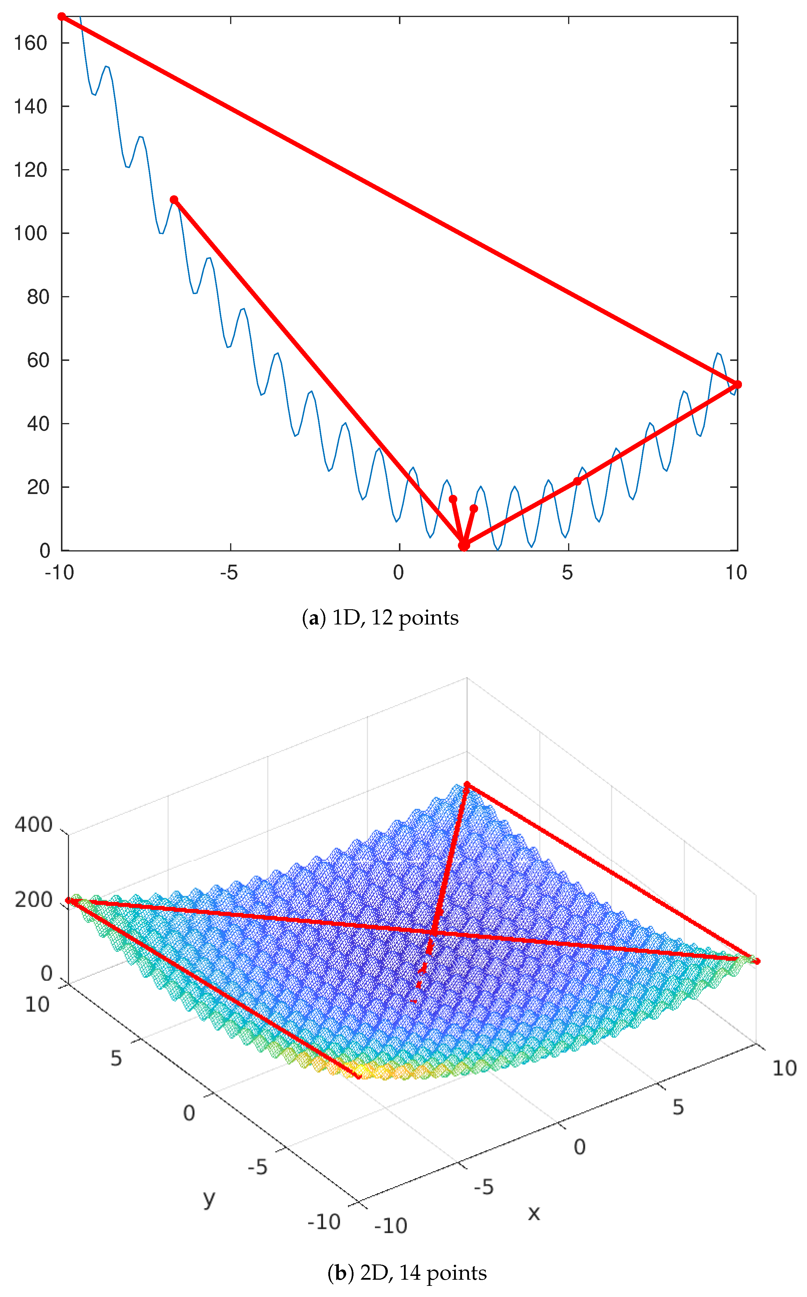
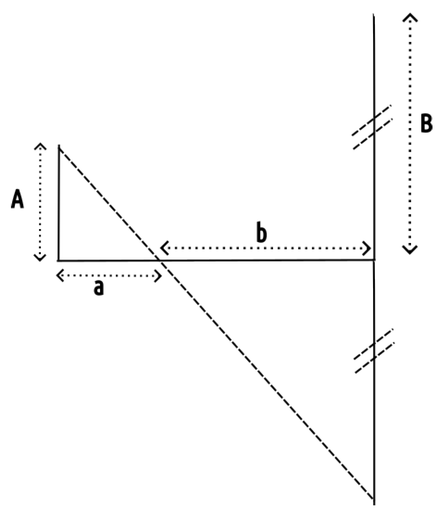
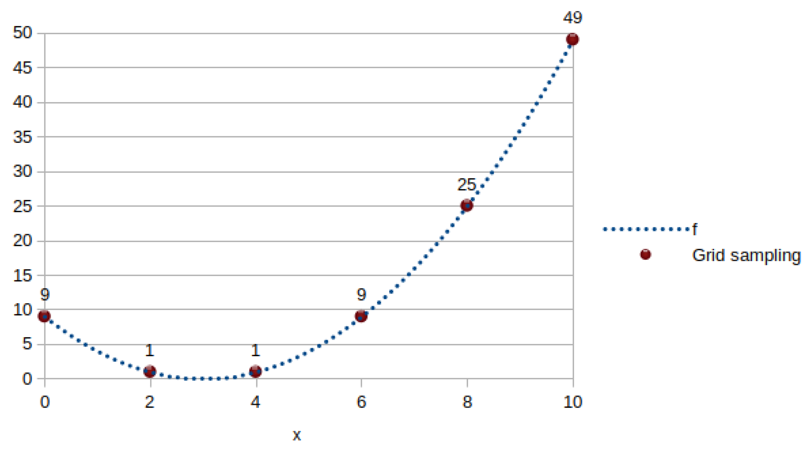
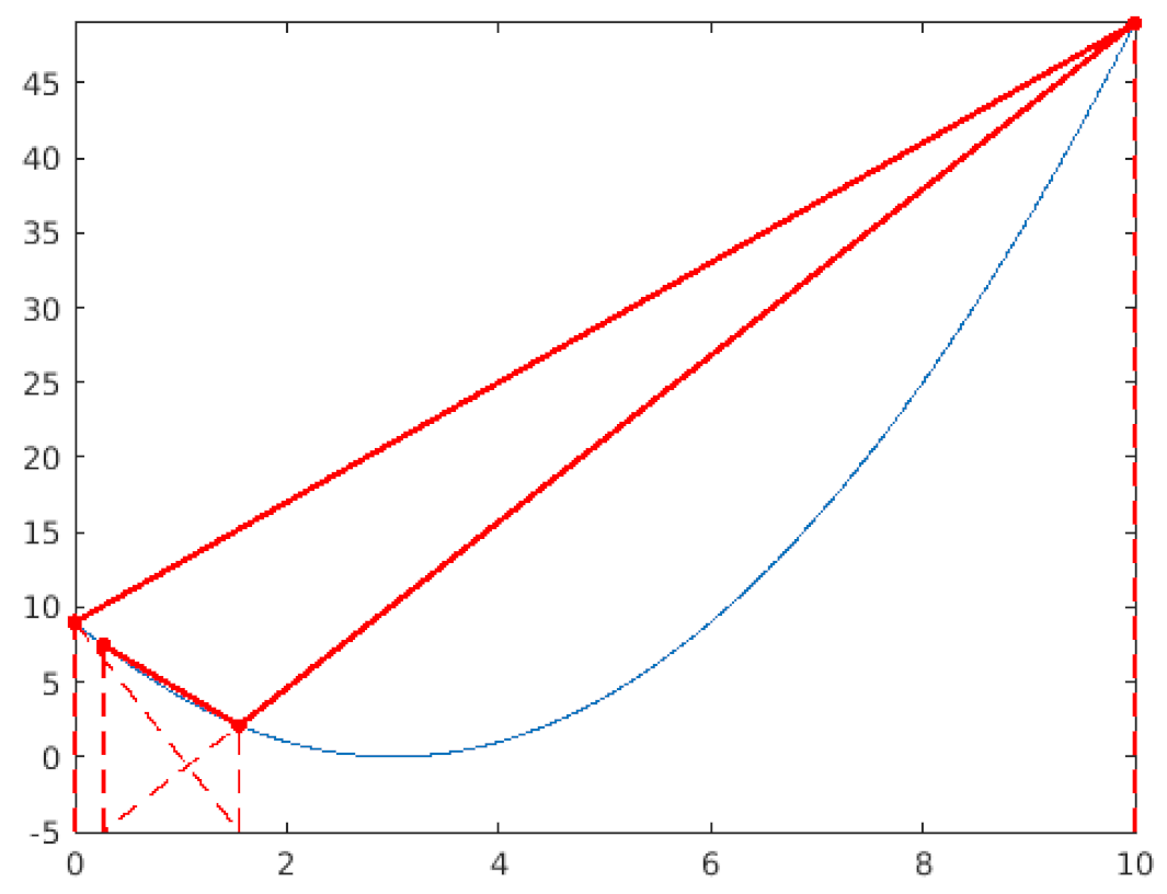
An horizontal lower bound is defined. The “corners” are evaluated. The line connecting them intersects the lower bound beyond the search space, this intersection point is rejected and will be replaced with another one (step 2).
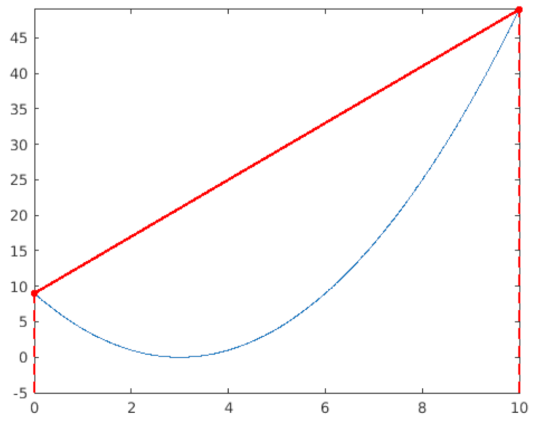
Mathematics 12 03755 i001
Table 3. Principle. Step 2.
The new position is defined so that a / b = A / B . As the dimension is 1, this can be achieved thanks to a “Ruler & Compass” construction. Then, the position is evaluated to define the third point.
Mathematics 12 03755 i002
Table 4. Principle. Step 3.
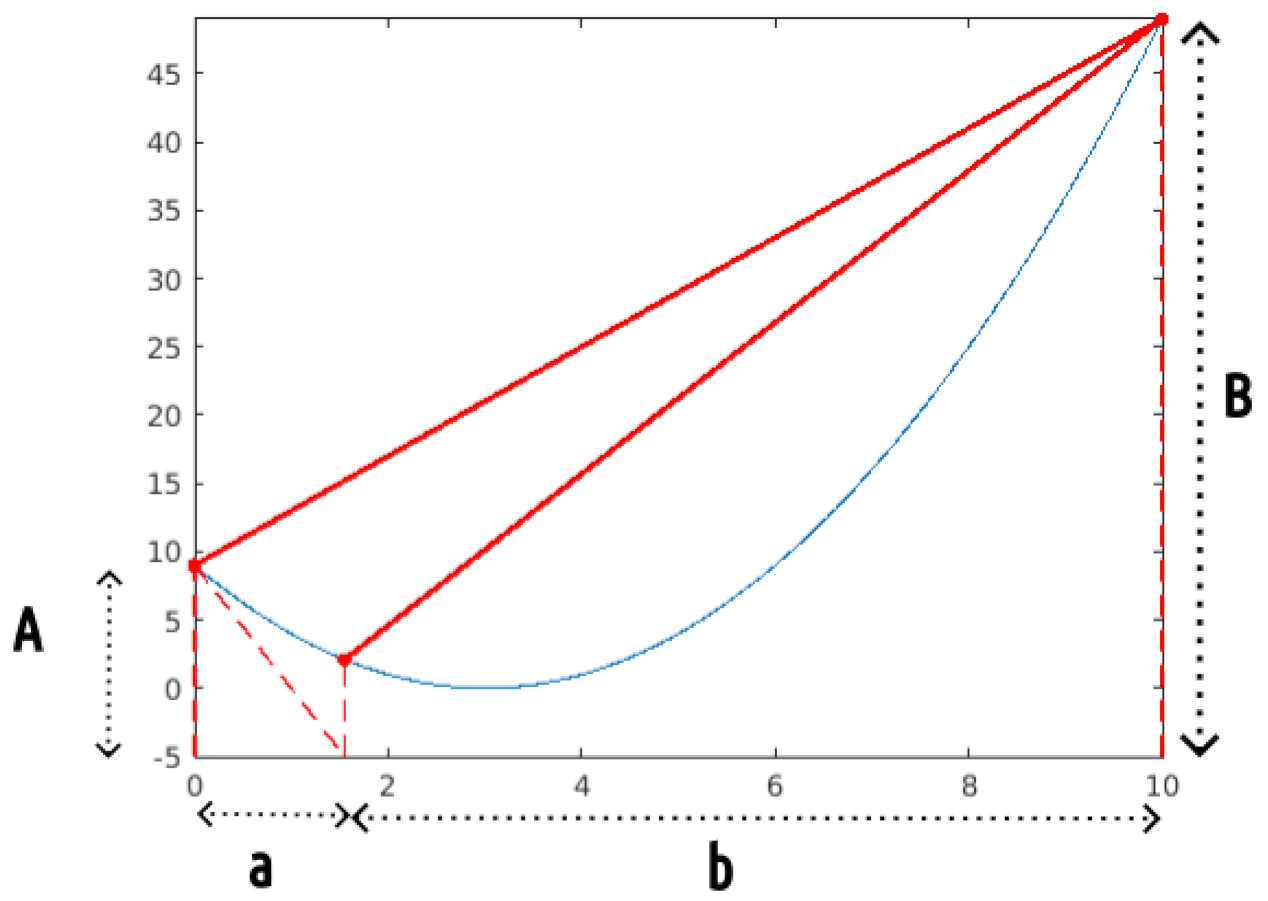
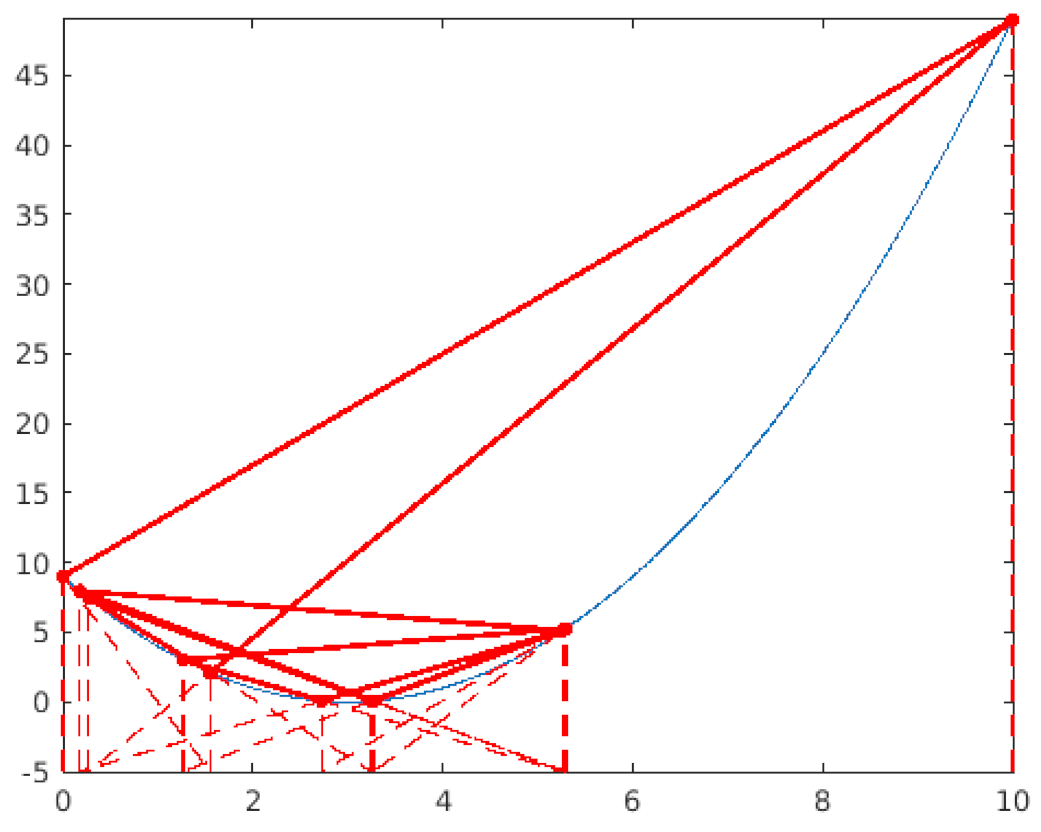
Now the line joining the two last points does intersect the lower bound on a point whose position is inside the search space. This position is then maintained and evaluated. The same process is repeated, again.
Mathematics 12 03755 i003
Table 5. Principle. Step 9, zoom.
… and again.
Mathematics 12 03755 i004
Table 6. Principle. Step 10, and zoom.
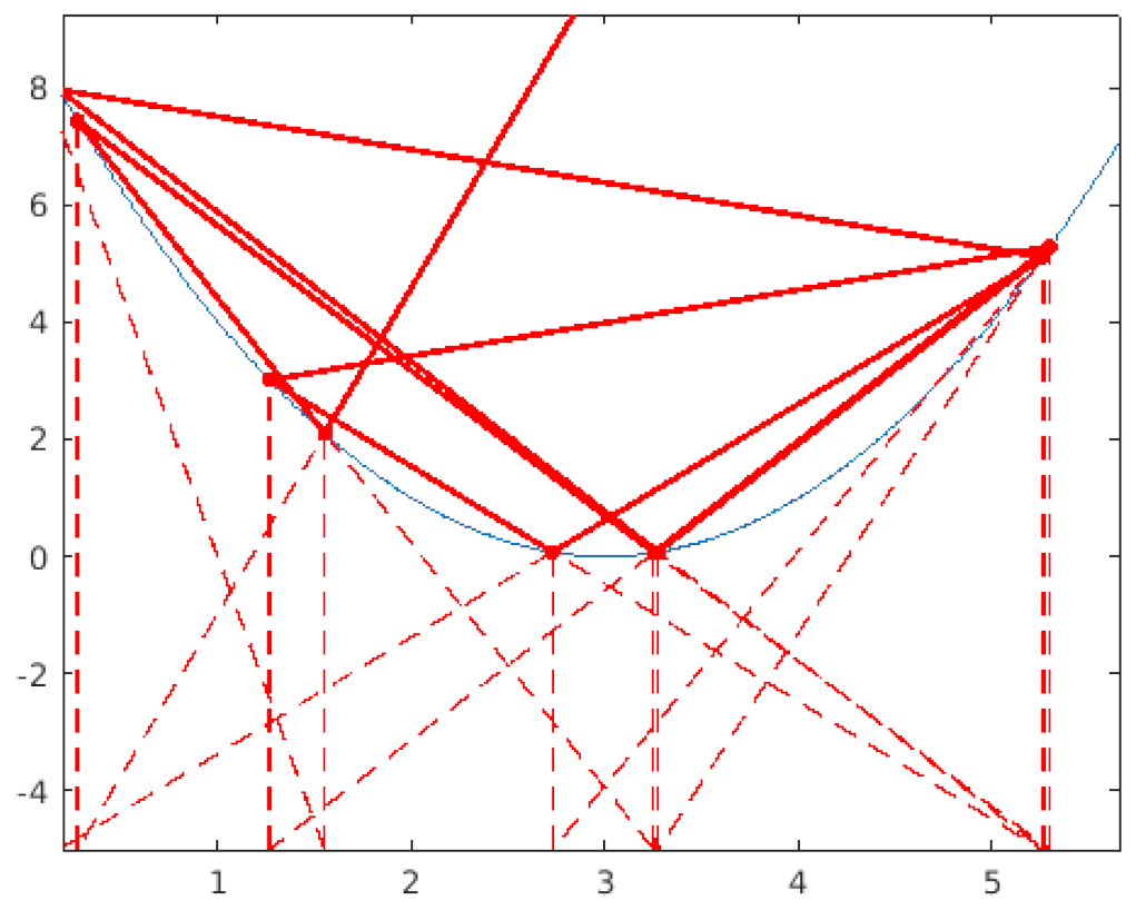
After Step 9, the line connecting the last two points is nearly horizontal and intersects the lower boundary outside of the search space. Consequently, we generate a new position using the same method as in Step 2. This occurrence becomes increasingly frequent as the positions approach the solution. Hence, the new position often approximates the mean of the last two positions, which is a favorable behavior for better approaching the solution.
Mathematics 12 03755 i005
Mathematics 12 03755 i006
Table 7. Six Hump Camel Back.
Constructed Points (Evaluations)Best Fitness
14−0.957541
24−1.030227
34−1.030227
44−1.031227
54−1.031227
64−1.031473
74−1.031473
84−1.031473
94−1.031473
104−1.031473
Table 8. Shifted Rastrigin.
DimensionConstructed Points (Evaluations)Best Fitness
1520.000557
210040.001511
315080.002548
450,0160.001735
5250,0320.004518
Table 9. Rosenbrock.
DimensionEvaluationsBest Fitness
22520.002788
315080.001003
410,0160.003756
515,0320.005719
Table 10. Pressure Vessel.
EvaluationsBest Fitness
105211,056.81
20496646.71
30746615.977
40746615.977
50746615.977
60766592.011
Table 11. Gear Train. Discretization is applied only at the very end to all values, so more search effort does not always imply a better result.
EvaluationsBest Fitness
116 3.10 × 10 3
130 1.20 × 10 3
173 6.65 × 10 9
223 6.65 × 10 9
1753 6.65 × 10 9
Table 12. RCO vs. PSO. The better values are highlighted in bold.
ProblemDimensionEvaluationsRCOPSO
Six Hump Camel Back254−1.031227−1.011030
Shifted Rastrigin1520.0005570.510724
210040.0015110.4397499
5250,0320.0045780.994959
10251,02435.2461.9899
Rosenbrock22520.002788266.94
515,0320.0057190.0864
10101,0248.996 5.19 × 10 8
Pressure Vessel430746615.9776890.347
50746615.9776821.931
20,0746583.756820.410
Gear Train4173 6.65 × 10 9 2.35 × 10 9
1154 6.65 × 10 9 2.35 × 10 9
199,752 1.18 × 10 9 1.26 × 10 9
Table 13. Computing time per iteration.
DimensionPlanesShifted Rastrigin
1 2.40 × 10 5 1.60 × 10 5
2 3.20 × 10 5 4.80 × 10 5
3 4.50 × 10 5 5.30 × 10 5
4 6.09 × 10 5 6.69 × 10 5
5 8.17 × 10 5 8.47 × 10 5
6 1.05 × 10 4 1.05 × 10 4
7 1.37 × 10 4 1.38 × 10 4
8 1.80 × 10 4 1.78 × 10 4
9 2.57 × 10 4 2.31 × 10 4
10 3.91 × 10 4 3.15 × 10 4
11 5.15 × 10 4 4.67 × 10 4
12 1.04 × 10 3 1.09 × 10 3
Disclaimer/Publisher’s Note: The statements, opinions and data contained in all publications are solely those of the individual author(s) and contributor(s) and not of MDPI and/or the editor(s). MDPI and/or the editor(s) disclaim responsibility for any injury to people or property resulting from any ideas, methods, instructions or products referred to in the content.

