
Enhanced Projection Method for the Solution of the System of Nonlinear Equations Under a More General Assumption than Pseudo-Monotonicity and Lipschitz Continuity


Abstract
1. Introduction
- 1.
- The article proposes an efficient algorithm for solving (1).
- 2.
- The operator F is assumed to satisfy a weaker condition than pseudo-monotonicity.
- 3.
- The proposed algorithm is globally convergent.
- 4.
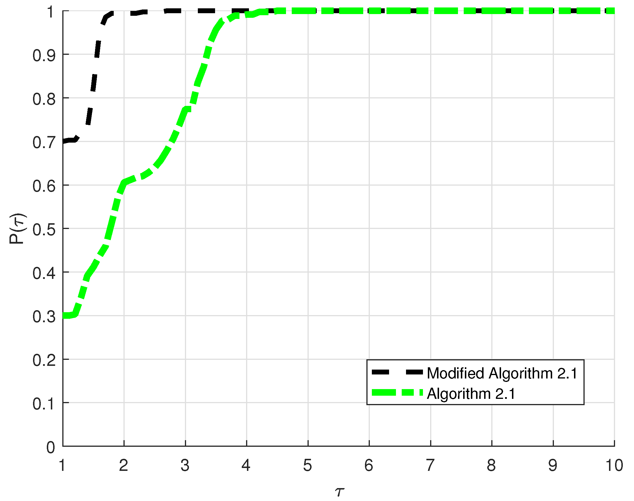
- On some test problems, which include monotone and pseudo-monotone, the proposed algorithm performs better than that of Liu et al. [8].
2. The Proposed Algorithm and Its Convergence
| Algorithm 1: (Modified Algorithm 2.1) |
Initialization. , , , , . Set Step 1. Evaluate , where the step size with i being the smallest non-negative integer satisfying
Step 2. Check if and stop. Else, evaluate
Step 3. Set and repeat the procedure. |
3. Numerical Experiments
3.1. Solving System of Monotone Equations
- Five dimensions:
- Seven initial points: , , , , , , .
- Parameters for Modified Algorithm 2.1: .
- The choice of is by trial and error in the interval and we got the best result at 1.7.
- Parameters for Algorithm 2.1: As chosen in [8].
- Stopping condition: when .
3.2. Solving Pseudo-Monotone Equations
4. Solving a Prediction Model
5. Conclusions
Author Contributions
Funding
Data Availability Statement
Acknowledgments
Conflicts of Interest
Appendix A
Appendix B

| Modified Algorithm 2.1 | Algorithm 2.1 | |||||||
|---|---|---|---|---|---|---|---|---|
| S/N | #ITN | #FEN | CPUTIMS | Norm | #ITN | #FEN | CPUTIMS | Norm |
| 1 | 27 | 32 | 0.012549 | 6.59 × | 43 | 45 | 0.007061 | 7.32 × |
| 2 | 13 | 17 | 0.005747 | 4.03 × | 26 | 28 | 0.006345 | 7.32 × |
| 3 | 11 | 15 | 0.003788 | 9.32 × | 26 | 28 | 0.006048 | 8.01 × |
| 4 | 7 | 11 | 0.003634 | 6.81 × | 20 | 22 | 0.004218 | 7.32 × |
| 5 | 11 | 15 | 0.009658 | 8.75 × | 32 | 34 | 0.009416 | 9.34 × |
| 6 | 9 | 13 | 0.003497 | 6.65 × | 25 | 27 | 0.004889 | 9.94 × |
| 7 | 9 | 13 | 0.00282 | 5.99 × | 24 | 26 | 0.00467 | 8.17 × |
| 8 | 22 | 27 | 0.025031 | 5.75 × | 41 | 43 | 0.036865 | 9.73 × |
| 9 | 10 | 14 | 0.011102 | 3.62 × | 24 | 26 | 0.018797 | 9.67 × |
| 10 | 7 | 11 | 0.008611 | 8.68 × | 25 | 27 | 0.021499 | 7.65 × |
| 11 | 7 | 11 | 0.009582 | 9.61 × | 18 | 20 | 0.015421 | 9.70 × |
| 12 | 11 | 15 | 0.012412 | 3.00 × | 31 | 33 | 0.026658 | 8.92 × |
| 13 | 9 | 13 | 0.011862 | 8.03 × | 24 | 26 | 0.021346 | 9.52 × |
| 14 | 9 | 13 | 0.010609 | 4.84 × | 22 | 24 | 0.020103 | 9.24 × |
| 15 | 19 | 24 | 0.039339 | 9.80 × | 41 | 43 | 0.060857 | 8.30 × |
| 16 | 9 | 13 | 0.019901 | 8.73 × | 24 | 26 | 0.032802 | 8.24 × |
| 17 | 10 | 14 | 0.019733 | 2.23 × | 24 | 26 | 0.042571 | 9.02 × |
| 18 | 7 | 11 | 0.014135 | 7.78 × | 18 | 20 | 0.030566 | 8.28 × |
| 19 | 11 | 15 | 0.023804 | 5.03 × | 31 | 33 | 0.048029 | 7.60 × |
| 20 | 9 | 13 | 0.018987 | 2.19 × | 24 | 26 | 0.037113 | 8.12 × |
| 21 | 8 | 12 | 0.017271 | 6.79 × | 22 | 24 | 0.034137 | 7.73 × |
| 22 | 16 | 21 | 0.10333 | 4.12 × | 40 | 42 | 0.23928 | 7.94 × |
| 23 | 8 | 12 | 0.071735 | 2.16 × | 23 | 25 | 0.12502 | 7.86 × |
| 24 | 9 | 13 | 0.076653 | 4.27 × | 23 | 25 | 0.15552 | 8.62 × |
| 25 | 9 | 13 | 0.073201 | 3.24 × | 17 | 19 | 0.11062 | 8.06 × |
| 26 | 9 | 13 | 0.079445 | 7.61 × | 30 | 32 | 0.19892 | 7.26 × |
| 27 | 11 | 15 | 0.092826 | 6.60 × | 23 | 25 | 0.14678 | 7.75 × |
| 28 | 10 | 14 | 0.088575 | 8.78 × | 21 | 23 | 0.13064 | 7.28 × |
| 29 | 15 | 20 | 0.25242 | 4.03 × | 39 | 41 | 0.44274 | 9.37 × |
| 30 | 10 | 14 | 0.14022 | 1.67 × | 22 | 24 | 0.26391 | 9.28 × |
| 31 | 10 | 14 | 0.15874 | 2.09 × | 23 | 25 | 0.28105 | 7.34 × |
| 32 | 9 | 13 | 0.13682 | 3.62 × | 16 | 18 | 0.2002 | 9.94 × |
| 33 | 10 | 14 | 0.17627 | 8.06 × | 29 | 31 | 0.3423 | 8.56 × |
| 34 | 12 | 16 | 0.20607 | 3.21 × | 22 | 24 | 0.24231 | 9.15 × |
| 35 | 12 | 16 | 0.2032 | 2.07 × | 20 | 22 | 0.24991 | 8.58 × |
| 36 | 7 | 8 | 0.00335 | 5.16 × | 10 | 10 | 0.006239 | 4.54 × |
| 37 | 6 | 7 | 0.002109 | 4.29 × | 10 | 10 | 0.002821 | 4.05 × |
| 38 | 6 | 7 | 0.002205 | 4.73 × | 10 | 10 | 0.002908 | 4.98 × |
| 39 | 8 | 8 | 0.002809 | 7.51 × | 9 | 9 | 0.003501 | 2.27 × |
| 40 | 6 | 7 | 0.002429 | 2.30 × | 11 | 11 | 0.003139 | 2.18 × |
| 41 | 6 | 7 | 0.002257 | 5.23 × | 10 | 10 | 0.002898 | 7.47 × |
| 42 | 6 | 7 | 0.002195 | 5.01 × | 10 | 10 | 0.00277 | 8.83 × |
| 43 | 7 | 8 | 0.008097 | 1.05 × | 11 | 11 | 0.009795 | 2.04 × |
| 44 | 6 | 7 | 0.007368 | 8.75 × | 10 | 10 | 0.010783 | 9.59 × |
| 45 | 6 | 7 | 0.006813 | 9.65 × | 11 | 11 | 0.012527 | 2.18 × |
| 46 | 5 | 6 | 0.006292 | 3.49 × | 9 | 9 | 0.009653 | 5.33 × |
| 47 | 6 | 7 | 0.007343 | 4.64 × | 11 | 11 | 0.01104 | 5.21 × |
| 48 | 6 | 7 | 0.00769 | 1.07 × | 11 | 11 | 0.014284 | 3.27 × |
| 49 | 6 | 7 | 0.007551 | 1.03 × | 11 | 11 | 0.011353 | 3.87 × |
| 50 | 7 | 8 | 0.015175 | 1.47 × | 11 | 11 | 0.016971 | 2.91 × |
| 51 | 6 | 7 | 0.012483 | 1.22 × | 11 | 11 | 0.017422 | 2.53 × |
| 52 | 6 | 7 | 0.014675 | 1.35 × | 11 | 11 | 0.019507 | 3.11 × |
| 53 | 5 | 6 | 0.013133 | 4.89 × | 9 | 9 | 0.014325 | 7.59 × |
| 54 | 6 | 7 | 0.013293 | 6.48 × | 11 | 11 | 0.017436 | 7.43 × |
| 55 | 6 | 7 | 0.012627 | 1.49 × | 11 | 11 | 0.018246 | 4.67 × |
| 56 | 6 | 7 | 0.012624 | 1.43 × | 11 | 11 | 0.018473 | 5.52 × |
| 57 | 7 | 8 | 0.060662 | 3.25 × | 11 | 11 | 0.065518 | 6.56 × |
| 58 | 6 | 7 | 0.053421 | 2.71 × | 11 | 11 | 0.07027 | 5.69 × |
| 59 | 6 | 7 | 0.047223 | 2.99 × | 11 | 11 | 0.072841 | 7.00 × |
| 60 | 6 | 7 | 0.045032 | 4.35 × | 10 | 10 | 0.06856 | 3.16 × |
| 61 | 7 | 8 | 0.050813 | 5.74 × | 12 | 12 | 0.079434 | 3.10 × |
| 62 | 6 | 7 | 0.057412 | 3.30 × | 12 | 12 | 0.085691 | 1.95 × |
| 63 | 6 | 7 | 0.052106 | 3.18 × | 12 | 12 | 0.079666 | 2.30 × |
| 64 | 7 | 8 | 0.095343 | 4.59 × | 11 | 11 | 0.14168 | 9.29 × |
| 65 | 6 | 7 | 0.1041 | 3.83 × | 11 | 11 | 0.14093 | 8.05 × |
| 66 | 6 | 7 | 0.096523 | 4.22 × | 11 | 11 | 0.15054 | 9.91 × |
| 67 | 6 | 7 | 0.1121 | 6.14 × | 10 | 10 | 0.13604 | 4.47 × |
| 68 | 7 | 8 | 0.11156 | 8.10 × | 12 | 12 | 0.16258 | 4.39 × |
| 69 | 6 | 7 | 0.1017 | 4.67 × | 12 | 12 | 0.17006 | 2.75 × |
| 70 | 6 | 7 | 0.10596 | 4.49 × | 12 | 12 | 0.15351 | 3.26 × |
| Modified Algorithm 2.1 | Algorithm 2.1 | |||||||
|---|---|---|---|---|---|---|---|---|
| S/N | #ITN | #FEN | CPUTIMS | Norm | #ITN | #FEN | CPUTIMS | Norm |
| 71 | 6 | 7 | 0.002304 | 3.45 × | 16 | 17 | 0.007615 | 9.47 × |
| 72 | 5 | 6 | 0.001865 | 3.11 × | 17 | 18 | 0.003803 | 4.96 × |
| 73 | 5 | 6 | 0.001603 | 3.79 × | 17 | 18 | 0.003723 | 6.17 × |
| 74 | 4 | 5 | 0.001902 | 8.09 × | 14 | 15 | 0.003143 | 6.60 × |
| 75 | 4 | 5 | 0.001797 | 5.03 × | 18 | 19 | 0.004189 | 7.98 × |
| 76 | 5 | 6 | 0.001817 | 5.44 × | 17 | 18 | 0.004069 | 9.62 × |
| 77 | 5 | 6 | 0.001741 | 6.08 × | 18 | 19 | 0.003914 | 4.97 × |
| 78 | 6 | 7 | 0.007113 | 7.71 × | 17 | 18 | 0.012589 | 8.97 × |
| 79 | 5 | 6 | 0.005826 | 6.95 × | 18 | 19 | 0.01471 | 4.70 × |
| 80 | 5 | 6 | 0.005458 | 8.49 × | 18 | 19 | 0.015735 | 5.84 × |
| 81 | 5 | 6 | 0.00603 | 7.24 × | 15 | 16 | 0.013362 | 6.25 × |
| 82 | 5 | 6 | 0.006419 | 4.50 × | 19 | 20 | 0.016425 | 7.56 × |
| 83 | 6 | 7 | 0.007573 | 4.87 × | 18 | 19 | 0.015699 | 9.11 × |
| 84 | 6 | 7 | 0.006383 | 5.44 × | 19 | 20 | 0.017787 | 4.71 × |
| 85 | 7 | 8 | 0.014922 | 4.36 × | 18 | 19 | 0.025146 | 5.37 × |
| 86 | 5 | 6 | 0.010037 | 9.83 × | 18 | 19 | 0.026788 | 6.65 × |
| 87 | 6 | 7 | 0.012495 | 4.80 × | 18 | 19 | 0.026249 | 8.26 × |
| 88 | 5 | 6 | 0.010712 | 1.02 × | 15 | 16 | 0.026128 | 8.84 × |
| 89 | 5 | 6 | 0.009591 | 6.36 × | 20 | 21 | 0.12091 | 4.53 × |
| 90 | 6 | 7 | 0.012814 | 6.88 × | 19 | 20 | 0.065515 | 5.46 × |
| 91 | 6 | 7 | 0.009786 | 7.69 × | 19 | 20 | 0.032207 | 6.66 × |
| 92 | 7 | 8 | 0.058986 | 9.76 × | 19 | 20 | 0.12435 | 5.09 × |
| 93 | 6 | 7 | 0.051312 | 8.79 × | 19 | 20 | 0.10918 | 6.30 × |
| 94 | 6 | 7 | 0.051025 | 1.07 × | 19 | 20 | 0.10658 | 7.83 × |
| 95 | 5 | 6 | 0.034137 | 2.29 × | 16 | 17 | 0.099565 | 8.37 × |
| 96 | 5 | 6 | 0.033763 | 1.42 × | 21 | 22 | 0.11681 | 4.29 × |
| 97 | 6 | 7 | 0.053704 | 1.54 × | 20 | 21 | 0.11358 | 5.17 × |
| 98 | 6 | 7 | 0.04435 | 1.72 × | 20 | 21 | 0.11402 | 6.31 × |
| 99 | 7 | 8 | 0.095347 | 1.38 × | 19 | 20 | 0.2194 | 7.20 × |
| 100 | 6 | 7 | 0.080087 | 1.24 × | 19 | 20 | 0.21158 | 8.91 × |
| 101 | 6 | 7 | 0.10761 | 1.52 × | 20 | 21 | 0.21943 | 4.69 × |
| 102 | 5 | 6 | 0.076939 | 3.24 × | 17 | 18 | 0.20373 | 5.01 × |
| 103 | 5 | 6 | 0.084055 | 2.01 × | 21 | 22 | 0.23125 | 6.06 × |
| 104 | 6 | 7 | 0.078271 | 2.18 × | 20 | 21 | 0.22096 | 7.31 × |
| 105 | 6 | 7 | 0.094979 | 2.43 × | 20 | 21 | 0.2237 | 8.92 × |
| 106 | 32 | 37 | 0.020347 | 7.96 × | 22 | 24 | 0.014247 | 6.06 × |
| 107 | 28 | 33 | 0.015387 | 6.01 × | 18 | 20 | 0.009144 | 9.09 × |
| 108 | 28 | 33 | 0.016649 | 7.52 × | 19 | 21 | 0.009963 | 5.72 × |
| 109 | 23 | 28 | 0.013364 | 7.52 × | 15 | 17 | 0.008333 | 6.96 × |
| 110 | 31 | 36 | 0.017272 | 6.59 × | 21 | 23 | 0.012308 | 6.01 × |
| 111 | 29 | 34 | 0.017474 | 7.23 × | 19 | 21 | 0.008633 | 9.15 × |
| 112 | 29 | 34 | 0.017756 | 9.04 × | 20 | 22 | 0.010131 | 5.79 × |
| 113 | 32 | 37 | 0.094368 | 8.13 × | 22 | 24 | 0.039793 | 5.80 × |
| 114 | 28 | 33 | 0.082168 | 6.15 × | 18 | 20 | 0.035767 | 8.78 × |
| 115 | 28 | 33 | 0.074468 | 7.68 × | 19 | 21 | 0.038823 | 5.52 × |
| 116 | 23 | 28 | 0.053698 | 7.69 × | 15 | 17 | 0.028847 | 7.00 × |
| 117 | 31 | 36 | 0.079769 | 6.74 × | 21 | 23 | 0.04158 | 5.71 × |
| 118 | 29 | 34 | 0.070896 | 7.39 × | 19 | 21 | 0.038367 | 8.83 × |
| 119 | 29 | 34 | 0.066047 | 9.24 × | 20 | 22 | 0.037947 | 5.55 × |
| 120 | 34 | 39 | 0.1496 | 8.94 × | 22 | 24 | 0.080009 | 5.83 × |
| 121 | 30 | 35 | 0.13246 | 6.70 × | 18 | 20 | 0.07721 | 8.97 × |
| 122 | 30 | 35 | 0.14889 | 8.38 × | 19 | 21 | 0.089545 | 5.61 × |
| 123 | 25 | 30 | 0.12179 | 8.42 × | 15 | 17 | 0.062893 | 7.38 × |
| 124 | 33 | 38 | 0.14733 | 7.35 × | 21 | 23 | 0.088768 | 5.73 × |
| 125 | 31 | 36 | 0.12906 | 8.12 × | 19 | 21 | 0.080111 | 8.97 × |
| 126 | 32 | 37 | 0.13739 | 6.16 × | 20 | 22 | 0.083265 | 5.61 × |
| 127 | 33 | 38 | 0.66309 | 9.95 × | 22 | 24 | 0.42308 | 6.45 × |
| 128 | 29 | 34 | 0.59025 | 7.46 × | 19 | 21 | 0.32225 | 5.30 × |
| 129 | 29 | 34 | 0.58551 | 9.33 × | 19 | 21 | 0.32422 | 6.63 × |
| 130 | 24 | 29 | 0.50665 | 9.41 × | 15 | 17 | 0.26425 | 9.52 × |
| 131 | 32 | 37 | 0.64034 | 8.18 × | 21 | 23 | 0.35608 | 6.45 × |
| 132 | 30 | 35 | 0.59725 | 9.04 × | 20 | 22 | 0.34836 | 5.20 × |
| 133 | 31 | 36 | 0.62419 | 6.86 × | 20 | 22 | 0.35536 | 6.50 × |
| 134 | 35 | 40 | 1.4228 | 6.54 × | 22 | 24 | 0.79544 | 7.04 × |
| 135 | 30 | 35 | 1.2619 | 8.22 × | 19 | 21 | 0.70235 | 5.96 × |
| 136 | 31 | 36 | 1.2791 | 6.16 × | 19 | 21 | 0.68651 | 7.45 × |
| 137 | 26 | 31 | 1.0565 | 6.12 × | 16 | 18 | 0.56092 | 5.27 × |
| 138 | 33 | 38 | 1.3681 | 9.05 × | 21 | 23 | 0.75447 | 7.12 × |
| 139 | 31 | 36 | 1.2819 | 9.85 × | 20 | 22 | 0.72687 | 5.80 × |
| 140 | 32 | 37 | 1.294 | 7.40 × | 20 | 22 | 0.70912 | 7.25 × |
| Modified Algorithm 2.1 | Algorithm 2.1 | |||||||
|---|---|---|---|---|---|---|---|---|
| S/N | #ITN | #FEN | CPUTIMS | Norm | #ITN | #FEN | CPUTIMS | Norm |
| 141 | 17 | 20 | 0.004937 | 4.52 × | 21 | 22 | 0.008009 | 9.50 × |
| 142 | 5 | 6 | 0.001713 | 7.90 × | 16 | 17 | 0.003245 | 8.03 × |
| 143 | 5 | 6 | 0.001649 | 2.37 × | 16 | 17 | 0.00312 | 8.87 × |
| 144 | 4 | 5 | 0.001521 | 7.09 × | 14 | 15 | 0.002874 | 6.38 × |
| 145 | 9 | 11 | 0.002973 | 4.71 × | 18 | 19 | 0.003675 | 7.72 × |
| 146 | 6 | 7 | 0.001804 | 4.71 × | 16 | 17 | 0.003099 | 8.59 × |
| 147 | 6 | 7 | 0.001752 | 9.45 × | 16 | 17 | 0.003163 | 5.99 × |
| 148 | 18 | 21 | 0.016777 | 3.90 × | 22 | 23 | 0.014803 | 8.99 × |
| 149 | 5 | 6 | 0.004776 | 1.77 × | 17 | 18 | 0.012174 | 7.61 × |
| 150 | 5 | 6 | 0.004689 | 5.29 × | 17 | 18 | 0.010071 | 8.40 × |
| 151 | 5 | 6 | 0.004853 | 6.34 × | 15 | 16 | 0.011069 | 6.04 × |
| 152 | 10 | 12 | 0.010422 | 2.44 × | 19 | 20 | 0.013393 | 7.31 × |
| 153 | 6 | 7 | 0.00621 | 1.05 × | 17 | 18 | 0.011774 | 8.14 × |
| 154 | 6 | 7 | 0.005477 | 2.11 × | 17 | 18 | 0.012273 | 5.68 × |
| 155 | 18 | 21 | 0.028969 | 5.51 × | 23 | 24 | 0.025267 | 5.39 × |
| 156 | 5 | 6 | 0.008543 | 2.50 × | 18 | 19 | 0.021878 | 4.56 × |
| 157 | 5 | 6 | 0.007935 | 7.48 × | 18 | 19 | 0.020262 | 5.03 × |
| 158 | 5 | 6 | 0.007635 | 8.97 × | 15 | 16 | 0.018653 | 8.55 × |
| 159 | 10 | 12 | 0.014168 | 3.46 × | 20 | 21 | 0.024233 | 4.38 × |
| 160 | 6 | 7 | 0.009346 | 1.49 × | 18 | 19 | 0.021854 | 4.87 × |
| 161 | 6 | 7 | 0.009303 | 2.99 × | 17 | 18 | 0.019861 | 8.03 × |
| 162 | 19 | 22 | 0.10679 | 4.75 × | 24 | 25 | 0.10954 | 5.10 × |
| 163 | 5 | 6 | 0.024869 | 5.59 × | 19 | 20 | 0.086488 | 4.32 × |
| 164 | 6 | 7 | 0.033129 | 6.69 × | 19 | 20 | 0.098119 | 4.77 × |
| 165 | 5 | 6 | 0.031583 | 2.01 × | 16 | 17 | 0.079964 | 8.10 × |
| 166 | 10 | 12 | 0.067059 | 7.73 × | 20 | 21 | 0.090297 | 9.79 × |
| 167 | 6 | 7 | 0.043345 | 3.33 × | 19 | 20 | 0.086513 | 4.62 × |
| 168 | 6 | 7 | 0.039999 | 6.69 × | 18 | 19 | 0.080409 | 7.60 × |
| 169 | 19 | 22 | 0.21191 | 6.72 × | 24 | 25 | 0.22354 | 7.22 × |
| 170 | 5 | 6 | 0.052672 | 7.90 × | 19 | 20 | 0.19205 | 6.11 × |
| 171 | 6 | 7 | 0.060095 | 9.46 × | 19 | 20 | 0.17649 | 6.74 × |
| 172 | 5 | 6 | 0.049432 | 2.84 × | 17 | 18 | 0.1556 | 4.85 × |
| 173 | 11 | 13 | 0.11165 | 2.54 × | 21 | 22 | 0.19498 | 5.87 × |
| 174 | 6 | 7 | 0.062295 | 4.71 × | 19 | 20 | 0.17683 | 6.53 × |
| 175 | 6 | 7 | 0.069349 | 9.45 × | 19 | 20 | 0.17397 | 4.55 × |
| 176 | 6 | 7 | 0.003274 | 2.21 × | 20 | 21 | 0.0099 | 6.54 × |
| 177 | 6 | 7 | 0.002565 | 3.36 × | 20 | 21 | 0.006416 | 9.96 × |
| 178 | 6 | 7 | 0.002542 | 3.33 × | 20 | 21 | 0.005817 | 9.86 × |
| 179 | 6 | 7 | 0.002521 | 3.48 × | 21 | 22 | 0.007736 | 4.36 × |
| 180 | 6 | 7 | 0.002729 | 2.85 × | 20 | 21 | 0.006059 | 8.44 × |
| 181 | 6 | 7 | 0.002552 | 3.23 × | 20 | 21 | 0.006105 | 9.58 × |
| 182 | 6 | 7 | 0.002597 | 3.17 × | 20 | 21 | 0.005912 | 9.39 × |
| 183 | 6 | 7 | 0.008548 | 4.97 × | 21 | 22 | 0.024977 | 6.20 × |
| 184 | 6 | 7 | 0.010067 | 7.58 × | 21 | 22 | 0.024948 | 9.45 × |
| 185 | 6 | 7 | 0.010134 | 7.51 × | 21 | 22 | 0.027187 | 9.36 × |
| 186 | 6 | 7 | 0.008447 | 7.84 × | 21 | 22 | 0.023051 | 9.78 × |
| 187 | 6 | 7 | 0.009162 | 6.42 × | 21 | 22 | 0.024516 | 8.01 × |
| 188 | 6 | 7 | 0.010227 | 7.29 × | 21 | 22 | 0.027204 | 9.09 × |
| 189 | 6 | 7 | 0.009605 | 7.15 × | 21 | 22 | 0.027912 | 8.91 × |
| 190 | 6 | 7 | 0.015264 | 7.04 × | 21 | 22 | 0.047974 | 8.78 × |
| 191 | 7 | 8 | 0.017883 | 4.29 × | 22 | 23 | 0.048759 | 5.66 × |
| 192 | 7 | 8 | 0.021565 | 4.25 × | 22 | 23 | 0.057282 | 5.61 × |
| 193 | 7 | 8 | 0.017947 | 4.44 × | 22 | 23 | 0.051161 | 5.86 × |
| 194 | 6 | 7 | 0.015928 | 9.09 × | 22 | 23 | 0.049698 | 4.80 × |
| 195 | 7 | 8 | 0.020241 | 4.13 × | 22 | 23 | 0.044966 | 5.45 × |
| 196 | 7 | 8 | 0.020234 | 4.04 × | 22 | 23 | 0.05325 | 5.34 × |
| 197 | 7 | 8 | 0.08097 | 6.30 × | 22 | 23 | 0.23407 | 8.31 × |
| 198 | 7 | 8 | 0.077386 | 9.59 × | 23 | 24 | 0.25148 | 5.37 × |
| 199 | 7 | 8 | 0.08756 | 9.50 × | 23 | 24 | 0.22674 | 5.31 × |
| 200 | 7 | 8 | 0.087484 | 9.92 × | 23 | 24 | 0.23848 | 5.55 × |
| 201 | 7 | 8 | 0.085698 | 8.13 × | 23 | 24 | 0.23279 | 4.55 × |
| 202 | 7 | 8 | 0.079353 | 9.23 × | 23 | 24 | 0.23078 | 5.16 × |
| 203 | 7 | 8 | 0.076134 | 9.04 × | 23 | 24 | 0.24152 | 5.06 × |
| 204 | 7 | 8 | 0.16516 | 8.90 × | 23 | 24 | 0.52592 | 4.98 × |
| 205 | 7 | 8 | 0.17342 | 1.36 × | 23 | 24 | 0.51509 | 7.59 × |
| 206 | 7 | 8 | 0.18053 | 1.34 × | 23 | 24 | 0.56798 | 7.52 × |
| 207 | 7 | 8 | 0.18972 | 1.40 × | 23 | 24 | 0.51232 | 7.85 × |
| 208 | 7 | 8 | 0.19649 | 1.15 × | 23 | 24 | 0.4876 | 6.43 × |
| 209 | 7 | 8 | 0.17832 | 1.30 × | 23 | 24 | 0.48184 | 7.30 × |
| 210 | 7 | 8 | 0.16083 | 1.28 × | 23 | 24 | 0.47876 | 7.15 × |
| Modified Algorithm 2.1 | Algorithm 2.1 | |||||||
|---|---|---|---|---|---|---|---|---|
| S/N | #ITN | #FEN | CPUTIMS | Norm | #ITN | #FEN | CPUTIMS | Norm |
| 211 | 7 | 11 | 0.002787 | 2.87 × | 18 | 20 | 0.010118 | 4.63 × |
| 212 | 9 | 12 | 0.002833 | 4.88 × | 13 | 14 | 0.00344 | 2.32 × |
| 213 | 9 | 12 | 0.002758 | 4.87 × | 12 | 13 | 0.002883 | 9.67 × |
| 214 | 9 | 12 | 0.003225 | 4.50 × | 13 | 14 | 0.003052 | 2.69 × |
| 215 | 8 | 11 | 0.00275 | 1.71 × | 14 | 16 | 0.003415 | 5.73 × |
| 216 | 9 | 12 | 0.002933 | 4.56 × | 12 | 13 | 0.00282 | 7.96 × |
| 217 | 9 | 12 | 0.002856 | 4.13 × | 12 | 13 | 0.002745 | 6.72 × |
| 218 | 7 | 11 | 0.008387 | 6.41 × | 19 | 21 | 0.01544 | 4.17 × |
| 219 | 10 | 13 | 0.010457 | 1.64 × | 13 | 14 | 0.014847 | 5.18 × |
| 220 | 10 | 13 | 0.01025 | 1.64 × | 13 | 14 | 0.011855 | 4.91 × |
| 221 | 10 | 13 | 0.010361 | 1.51 × | 13 | 14 | 0.014554 | 6.03 × |
| 222 | 8 | 11 | 0.009885 | 3.82 × | 15 | 17 | 0.014416 | 5.16 × |
| 223 | 10 | 13 | 0.011475 | 1.53 × | 13 | 14 | 0.010824 | 4.05 × |
| 224 | 9 | 12 | 0.009921 | 9.23 × | 13 | 14 | 0.010405 | 3.41 × |
| 225 | 7 | 11 | 0.015621 | 9.07 × | 19 | 21 | 0.024918 | 5.89 × |
| 226 | 10 | 13 | 0.017874 | 2.32 × | 13 | 14 | 0.019826 | 7.33 × |
| 227 | 10 | 13 | 0.017879 | 2.32 × | 13 | 14 | 0.01944 | 6.95 × |
| 228 | 10 | 13 | 0.016985 | 2.14 × | 13 | 14 | 0.017264 | 8.52 × |
| 229 | 8 | 11 | 0.017064 | 5.41 × | 15 | 17 | 0.020474 | 7.30 × |
| 230 | 10 | 13 | 0.021175 | 2.17 × | 13 | 14 | 0.020304 | 5.72 × |
| 231 | 10 | 13 | 0.022681 | 1.96 × | 13 | 14 | 0.018144 | 4.83 × |
| 232 | 8 | 12 | 0.074286 | 1.62 × | 20 | 22 | 0.1296 | 5.31 × |
| 233 | 10 | 13 | 0.086261 | 5.19 × | 14 | 15 | 0.074373 | 3.72 × |
| 234 | 10 | 13 | 0.085189 | 5.18 × | 14 | 15 | 0.075556 | 3.53 × |
| 235 | 10 | 13 | 0.070252 | 4.79 × | 14 | 15 | 0.097656 | 4.33 × |
| 236 | 9 | 12 | 0.061971 | 1.82 × | 16 | 18 | 0.11044 | 6.57 × |
| 237 | 10 | 13 | 0.072558 | 4.85 × | 14 | 15 | 0.078055 | 2.91 × |
| 238 | 10 | 13 | 0.072285 | 4.39 × | 14 | 15 | 0.085565 | 2.45 × |
| 239 | 8 | 12 | 0.1303 | 2.29 × | 20 | 22 | 0.24278 | 7.51 × |
| 240 | 10 | 13 | 0.13622 | 7.33 × | 14 | 15 | 0.14111 | 5.26 × |
| 241 | 10 | 13 | 0.13184 | 7.32 × | 14 | 15 | 0.16725 | 4.99 × |
| 242 | 10 | 13 | 0.15374 | 6.77 × | 14 | 15 | 0.15677 | 6.12 × |
| 243 | 9 | 12 | 0.12203 | 2.57 × | 16 | 18 | 0.19677 | 9.29 × |
| 244 | 10 | 13 | 0.12991 | 6.85 × | 14 | 15 | 0.16913 | 4.11 × |
| 245 | 10 | 13 | 0.13898 | 6.21 × | 14 | 15 | 0.17488 | 3.47 × |
| 246 | 47 | 53 | 0.013743 | 8.15 × | 37 | 39 | 0.013714 | 9.08 × |
| 247 | 51 | 57 | 0.013771 | 6.94 × | 34 | 36 | 0.0082 | 6.34 × |
| 248 | 49 | 55 | 0.013174 | 8.89 × | 33 | 35 | 0.00843 | 9.02 × |
| 249 | 43 | 49 | 0.012099 | 9.14 × | 34 | 36 | 0.007969 | 9.82 × |
| 250 | 39 | 45 | 0.01061 | 8.97 × | 24 | 27 | 0.006147 | 8.48 × |
| 251 | 50 | 56 | 0.013017 | 9.10 × | 32 | 34 | 0.007422 | 8.19 × |
| 252 | 48 | 54 | 0.01351 | 7.91 × | 31 | 33 | 0.007473 | 6.91 × |
| 253 | 49 | 55 | 0.048504 | 9.24 × | 38 | 40 | 0.030185 | 8.37 × |
| 254 | 51 | 57 | 0.051623 | 9.04 × | 34 | 36 | 0.028671 | 7.98 × |
| 255 | 52 | 58 | 0.055527 | 7.82 × | 33 | 35 | 0.031817 | 7.71 × |
| 256 | 44 | 50 | 0.046667 | 7.33 × | 35 | 37 | 0.030614 | 6.94 × |
| 257 | 40 | 46 | 0.047911 | 8.29 × | 25 | 28 | 0.024683 | 8.52 × |
| 258 | 50 | 56 | 0.052069 | 6.95 × | 33 | 35 | 0.031479 | 6.86 × |
| 259 | 51 | 57 | 0.057943 | 7.07 × | 31 | 33 | 0.032096 | 9.41 × |
| 260 | 49 | 55 | 0.093172 | 9.56 × | 37 | 39 | 0.063399 | 9.06 × |
| 261 | 53 | 59 | 0.10543 | 7.07 × | 33 | 35 | 0.058766 | 8.70 × |
| 262 | 52 | 58 | 0.094878 | 8.57 × | 33 | 35 | 0.056938 | 9.10 × |
| 263 | 45 | 51 | 0.099841 | 8.27 × | 35 | 37 | 0.059072 | 5.78 × |
| 264 | 42 | 48 | 0.077874 | 7.18 × | 16 | 19 | 0.031977 | 7.17 × |
| 265 | 49 | 55 | 0.10448 | 9.72 × | 32 | 34 | 0.057166 | 8.37 × |
| 266 | 51 | 57 | 0.096876 | 7.82 × | 32 | 34 | 0.052285 | 7.18 × |
| 267 | 48 | 54 | 0.42402 | 9.25 × | 44 | 46 | 0.33999 | 8.69 × |
| 268 | 54 | 60 | 0.48368 | 8.64 × | 34 | 36 | 0.26149 | 6.01 × |
| 269 | 52 | 58 | 0.47291 | 8.54 × | 34 | 36 | 0.25476 | 6.15 × |
| 270 | 45 | 51 | 0.39962 | 8.20 × | 35 | 37 | 0.28283 | 9.76 × |
| 271 | 46 | 52 | 0.41143 | 7.04 × | 20 | 23 | 0.15533 | 9.29 × |
| 272 | 53 | 59 | 0.46859 | 8.28 × | 33 | 35 | 0.26206 | 5.90 × |
| 273 | 52 | 58 | 0.46464 | 9.22 × | 32 | 34 | 0.23148 | 8.85 × |
| 274 | 49 | 55 | 0.94845 | 8.90 × | 38 | 40 | 0.57732 | 6.68 × |
| 275 | 54 | 60 | 0.97398 | 9.02 × | 35 | 37 | 0.58925 | 9.39 × |
| 276 | 51 | 57 | 0.94823 | 8.51 × | 35 | 37 | 0.56687 | 6.82 × |
| 277 | 45 | 51 | 0.81796 | 9.20 × | 34 | 36 | 0.67887 | 9.27 × |
| 278 | 45 | 51 | 0.81929 | 8.11 × | 29 | 31 | 0.51234 | 8.85 × |
| 279 | 52 | 58 | 0.97168 | 7.44 × | 34 | 36 | 0.51023 | 7.71 × |
| 280 | 51 | 57 | 0.96547 | 9.76 × | 32 | 34 | 0.54492 | 9.94 × |
| Modified Algorithm 2.1 | Algorithm 2.1 | |||||||
|---|---|---|---|---|---|---|---|---|
| S/N | #ITN | #FEN | CPUTIMS | Norm | #ITN | #FEN | CPUTIMS | Norm |
| 281 | 10 | 15 | 0.006116 | 2.50 × | 28 | 32 | 0.012731 | 9.50 × |
| 282 | 4 | 12 | 0.003065 | 1.52 × | 7 | 10 | 0.00344 | 8.84 × |
| 283 | 4 | 12 | 0.003011 | 1.85 × | 7 | 10 | 0.002849 | 1.23 × |
| 284 | 3 | 11 | 0.002896 | 7.36 × | 6 | 9 | 0.002484 | 1.28 × |
| 285 | 9 | 14 | 0.005233 | 3.84 × | 25 | 26 | 0.010551 | 7.49 × |
| 286 | 4 | 12 | 0.002981 | 1.11 × | 7 | 10 | 0.002695 | 2.77 × |
| 287 | 4 | 12 | 0.0034 | 6.46 × | 7 | 10 | 0.002708 | 4.42 × |
| 288 | 10 | 15 | 0.021468 | 5.60 × | 30 | 34 | 0.037754 | 6.19 × |
| 289 | 4 | 12 | 0.009983 | 3.41 × | 7 | 10 | 0.010639 | 1.98 × |
| 290 | 4 | 12 | 0.011755 | 4.14 × | 7 | 10 | 0.008466 | 2.75 × |
| 291 | 4 | 12 | 0.011676 | 1.09 × | 6 | 9 | 0.009563 | 2.85 × |
| 292 | 9 | 14 | 0.021063 | 8.59 × | 26 | 27 | 0.039797 | 8.78 × |
| 293 | 4 | 12 | 0.011692 | 2.48 × | 7 | 10 | 0.010779 | 6.20 × |
| 294 | 5 | 13 | 0.01184 | 9.58 × | 7 | 10 | 0.010062 | 9.87 × |
| 295 | 10 | 15 | 0.046832 | 7.92 × | 30 | 34 | 0.066245 | 8.75 × |
| 296 | 4 | 12 | 0.019588 | 4.82 × | 7 | 10 | 0.017993 | 2.79 × |
| 297 | 4 | 12 | 0.019449 | 5.85 × | 7 | 10 | 0.017382 | 3.89 × |
| 298 | 4 | 12 | 0.018484 | 1.54 × | 6 | 9 | 0.015333 | 4.03 × |
| 299 | 10 | 15 | 0.042982 | 1.40 × | 27 | 28 | 0.081366 | 6.51 × |
| 300 | 4 | 12 | 0.020116 | 3.51 × | 7 | 10 | 0.019162 | 8.77 × |
| 301 | 5 | 13 | 0.022106 | 1.35 × | 8 | 11 | 0.021451 | 6.77 × |
| 302 | 11 | 16 | 0.18611 | 2.14 × | 32 | 36 | 0.30956 | 5.70 × |
| 303 | 5 | 13 | 0.085259 | 7.15 × | 7 | 10 | 0.071141 | 6.25 × |
| 304 | 5 | 13 | 0.086118 | 8.68 × | 7 | 10 | 0.070638 | 8.70 × |
| 305 | 4 | 12 | 0.066601 | 3.45 × | 6 | 9 | 0.068205 | 9.02 × |
| 306 | 10 | 15 | 0.1791 | 3.13 × | 28 | 29 | 0.36233 | 7.63 × |
| 307 | 4 | 12 | 0.073026 | 7.84 × | 8 | 11 | 0.07243 | 9.52 × |
| 308 | 5 | 13 | 0.094781 | 3.03 × | 8 | 11 | 0.076468 | 1.51 × |
| 309 | 11 | 16 | 0.37098 | 3.02 × | 32 | 36 | 0.57126 | 8.06 × |
| 310 | 5 | 13 | 0.16142 | 1.01 × | 7 | 10 | 0.14156 | 8.84 × |
| 311 | 5 | 13 | 0.16726 | 1.23 × | 8 | 11 | 0.1627 | 5.97 × |
| 312 | 4 | 12 | 0.15383 | 4.88 × | 7 | 10 | 0.14542 | 6.19 × |
| 313 | 10 | 15 | 0.33181 | 4.42 × | 29 | 30 | 0.76471 | 5.66 × |
| 314 | 4 | 12 | 0.1434 | 1.11 × | 8 | 11 | 0.16435 | 1.35 × |
| 315 | 5 | 13 | 0.16446 | 4.28 × | 8 | 11 | 0.15826 | 2.14 × |
| 316 | 9 | 14 | 0.002652 | 1.63 × | 6 | 8 | 0.005616 | 1.91 × |
| 317 | 8 | 13 | 0.00223 | 5.69 × | 5 | 7 | 0.001373 | 4.71 × |
| 318 | 8 | 13 | 0.002088 | 5.13 × | 5 | 7 | 0.001319 | 4.25 × |
| 319 | 8 | 13 | 0.002094 | 7.71 × | 5 | 7 | 0.001329 | 6.39 × |
| 320 | 8 | 13 | 0.002334 | 3.29 × | 5 | 7 | 0.001555 | 2.72 × |
| 321 | 8 | 13 | 0.002117 | 3.45 × | 5 | 7 | 0.001348 | 2.85 × |
| 322 | 8 | 13 | 0.002049 | 2.32 × | 5 | 7 | 0.001393 | 1.92 × |
| 323 | 9 | 14 | 0.005421 | 3.64 × | 6 | 8 | 0.00313 | 4.27 × |
| 324 | 9 | 14 | 0.005392 | 1.43 × | 6 | 8 | 0.003146 | 1.67 × |
| 325 | 9 | 14 | 0.004636 | 1.29 × | 5 | 7 | 0.002823 | 9.50 × |
| 326 | 9 | 14 | 0.006621 | 1.93 × | 6 | 8 | 0.003147 | 2.27 × |
| 327 | 8 | 13 | 0.005317 | 7.35 × | 5 | 7 | 0.002791 | 6.09 × |
| 328 | 8 | 13 | 0.004959 | 7.70 × | 5 | 7 | 0.002797 | 6.38 × |
| 329 | 8 | 13 | 0.005101 | 5.20 × | 5 | 7 | 0.002815 | 4.30 × |
| 330 | 9 | 14 | 0.009009 | 5.15 × | 6 | 8 | 0.005518 | 6.04 × |
| 331 | 9 | 14 | 0.009207 | 2.02 × | 6 | 8 | 0.005216 | 2.37 × |
| 332 | 9 | 14 | 0.009298 | 1.82 × | 6 | 8 | 0.00609 | 2.13 × |
| 333 | 9 | 14 | 0.010277 | 2.73 × | 6 | 8 | 0.005403 | 3.21 × |
| 334 | 9 | 14 | 0.008843 | 1.17 × | 5 | 7 | 0.006774 | 8.61 × |
| 335 | 9 | 14 | 0.012841 | 1.22 × | 5 | 7 | 0.005742 | 9.03 × |
| 336 | 8 | 13 | 0.008488 | 7.35 × | 5 | 7 | 0.005547 | 6.09 × |
| 337 | 10 | 15 | 0.052058 | 1.29 × | 6 | 8 | 0.024152 | 1.35 × |
| 338 | 9 | 14 | 0.046709 | 4.51 × | 6 | 8 | 0.027561 | 5.29 × |
| 339 | 9 | 14 | 0.045669 | 4.07 × | 6 | 8 | 0.022766 | 4.77 × |
| 340 | 9 | 14 | 0.041849 | 6.11 × | 6 | 8 | 0.027313 | 7.17 × |
| 341 | 9 | 14 | 0.045016 | 2.61 × | 6 | 8 | 0.024754 | 3.06 × |
| 342 | 9 | 14 | 0.041722 | 2.73 × | 6 | 8 | 0.02272 | 3.21 × |
| 343 | 9 | 14 | 0.040575 | 1.84 × | 6 | 8 | 0.026991 | 2.16 × |
| 344 | 10 | 15 | 0.098303 | 1.83 × | 6 | 8 | 0.0526 | 1.91 × |
| 345 | 9 | 14 | 0.1109 | 6.38 × | 6 | 8 | 0.048555 | 7.49 × |
| 346 | 9 | 14 | 0.092654 | 5.75 × | 6 | 8 | 0.049859 | 6.75 × |
| 347 | 9 | 14 | 0.088206 | 8.65 × | 6 | 8 | 0.048326 | 1.01 × |
| 348 | 9 | 14 | 0.094452 | 3.69 × | 6 | 8 | 0.049995 | 4.32 × |
| 349 | 9 | 14 | 0.088618 | 3.86 × | 6 | 8 | 0.056488 | 4.53 × |
| 350 | 9 | 14 | 0.099802 | 2.61 × | 6 | 8 | 0.04795 | 3.06 × |
References
- Abdullahi, M.; Abubakar, A.B.; Feng, Y.; Liu, J. Comment on: “A derivative-free iterative method for nonlinear monotone equations with convex constraints”. Numer. Algorithms 2023, 94, 1551–1560. [Google Scholar] [CrossRef]
- Wang, C.; Wang, Y. A superlinearly convergent projection method for constrained systems of nonlinear equations. J. Glob. Optim. 2009, 44, 283–296. [Google Scholar] [CrossRef]
- Ibrahim, A.H.; Kumam, P.; Abubakar, A.B.; Abubakar, J.; Muhammad, A.B. Least-Square-Based Three-Term Conjugate Gradient Projection Method for ℓ1-Norm Problems with Application to Compressed Sensing. Mathematics 2020, 8, 602. [Google Scholar] [CrossRef]
- Hager, W.; Zhang, H. A New Conjugate Gradient Method with Guaranteed Descent and an Efficient Line Search. SIAM J. Optim. 2005, 16, 170–192. [Google Scholar] [CrossRef]
- Liu, J.K.; Feng, Y. A derivative-free iterative method for nonlinear monotone equations with convex constraints. Numer. Algorithms 2018, 82, 245–262. [Google Scholar] [CrossRef]
- Gao, P.; He, C. An efficient three-term conjugate gradient method for nonlinear monotone equations with convex constraints. Calcolo 2018, 55, 53. [Google Scholar] [CrossRef]
- Cruz, W.L. A spectral algorithm for large-scale systems of nonlinear monotone equations. Numer. Algorithms 2017, 76, 1109–1130. [Google Scholar] [CrossRef]
- Liu, J.; Lu, Z.; Xu, J.; Wu, S.; Tu, Z. An efficient projection-based algorithm without Lipschitz continuity for large-scale nonlinear pseudo-monotone equations. J. Comput. Appl. Math. 2022, 403, 113822. [Google Scholar] [CrossRef]
- Awwal, A.M.; Botmart, T. A new sufficiently descent algorithm for pseudomonotone nonlinear operator equations and signal reconstruction. Numer. Algorithms 2023, 94, 1125–1158. [Google Scholar] [CrossRef]
- Dolan, E.D.; Moré, J.J. Benchmarking optimization software with performance profiles. Math. Program. 2002, 91, 201–213. [Google Scholar] [CrossRef]
- Shehu, Y.; Dong, Q.; Jiang, D. Single projection method for pseudo-monotone variational inequality in Hilbert spaces. Optimization 2019, 68, 385–409. [Google Scholar] [CrossRef]
- Thong, D.V.; Vuong, P.T. R-linear convergence analysis of inertial extragradient algorithms for strongly pseudo-monotone variational inequalities. J. Comput. Appl. Math. 2022, 406, 114003. [Google Scholar] [CrossRef]
- Jin, X.; Zhang, X.; Huang, K.; Geng, G. Stochastic Conjugate Gradient Algorithm With Variance Reduction. IEEE Trans. Neural Netw. Learn. Syst. 2019, 30, 1360–1369. [Google Scholar] [CrossRef] [PubMed]
- Jian, J.; Yin, J.; Tang, C.; Han, D. A family of inertial derivative-free projection methods for constrained nonlinear pseudo-monotone equations with applications. Comput. Appl. Math. 2022, 41, 309. [Google Scholar] [CrossRef]
- Liu, W.; Jian, J.; Yin, J. An inertial spectral conjugate gradient projection method for constrained nonlinear pseudo-monotone equations. Numer. Algorithms 2024, 97, 985–1015. [Google Scholar] [CrossRef]
- Koorapetse, M.; Kaelo, P.; Lekoko, S.; Diphofu, T. A derivative-free RMIL conjugate gradient projection method for convex constrained nonlinear monotone equations with applications in compressive sensing. Appl. Numer. Math. 2021, 165, 431–441. [Google Scholar] [CrossRef]
- Chang, C.; Lin, C. LIBSVM: A library for support vector machines. ACM Trans. Intell. Syst. Technol. (TIST) 2011, 2, 1–27. [Google Scholar] [CrossRef]
- La Cruz, W.; Martínez, J.; Raydan, M. Spectral residual method without gradient information for solving large-scale nonlinear systems of equations. Math. Comput. 2006, 75, 1429–1448. [Google Scholar] [CrossRef]
- Yu, Z.; Lin, J.; Sun, J.; Xiao, Y.H.; Liu, L.Y.; Li, Z.H. Spectral gradient projection method for monotone nonlinear equations with convex constraints. Appl. Numer. Math. 2009, 59, 2416–2423. [Google Scholar] [CrossRef]
- Li, Q.; Li, D. A class of derivative-free methods for large-scale nonlinear monotone equations. IMA J. Numer. Anal. 2011, 31, 1625–1635. [Google Scholar] [CrossRef]
- Zhou, W.; Li, D. Limited memory BFGS method for nonlinear monotone equations. J. Comput. Math. 2007, 25, 89–96. [Google Scholar]
- Abubakar, A.B.; Kumam, P.; Mohammad, H.; Ibrahim, A.H.; Kiri, A.I. A hybrid approach for finding approximate solutions to constrained nonlinear monotone operator equations with applications. Appl. Numer. Math. 2022, 177, 79–92. [Google Scholar] [CrossRef]


| Modified Algorithm 2.1 | Algorithm 2.1 | ||||||||
|---|---|---|---|---|---|---|---|---|---|
| Problem | Initial Point | #ITN | #FEN | CPUTIMS | Norm | #ITN | #FEN | CPUTIMS | Norm |
| P1 | (0,0) | 17 | 17 | 0.008397 | 4.48 × | 34 | 34 | 0.002663 | 7.95 × |
| 18 | 18 | 0.006964 | 7.19 × | 36 | 36 | 0.00257 | 7.75 × | ||
| 17 | 17 | 0.004736 | 7.44 × | 34 | 34 | 0.002293 | 9.13 × | ||
| 16 | 16 | 0.002552 | 9.75 × | 34 | 34 | 0.002786 | 6.46 × | ||
| 16 | 16 | 0.004537 | 8.75 × | 34 | 34 | 0.002557 | 7.00 × | ||
| P2 | (0.2,0.2,0.2) | 60 | 66 | 0.017991 | 9.63 × | 98 | 100 | 0.009262 | 8.98 × |
| 61 | 67 | 0.00344 | 8.96 × | 102 | 104 | 0.005058 | 9.73 × | ||
| 55 | 61 | 0.003559 | 9.53 × | 69 | 71 | 0.003775 | 9.38 × | ||
| 75 | 81 | 0.004154 | 9.09 × | 85 | 87 | 0.004471 | 9.81 × | ||
| 78 | 84 | 0.004725 | 9.26 × | 56 | 57 | 0.0036 | 9.75 × | ||
| S/N | Dataset | Data Points N | Number of Variables n |
|---|---|---|---|
| 1 | a1a.t | 30,956 | 123 |
| 2 | a2a.t | 30,296 | 123 |
| 3 | a3a.t | 29,376 | 123 |
| 4 | a4a.t | 27,780 | 123 |
| 5 | a5a.t | 26,147 | 123 |
| 6 | a6a.t | 21,341 | 123 |
| 7 | colon-cancer | 62 | 2000 |
| 8 | svmguide1.t | 4000 | 4 |
| 9 | svmguide4.t | 312 | 10 |
| 10 | usps.t | 2007 | 256 |
| DFMRMIL | Algorithm 2.1 | Modified Algorithm 2.1 | |
|---|---|---|---|
| S/N | #ITN/#FEN/CPUTIMS/Norm | #ITN/#FEN/CPUTIMS/Norm | #ITN/#FEN/CPUTIMS/Norm |
| 1 | 715.2/1430.6/7.709/9.92 × | 172.4/345.4/1.881/9.86 × | 116.4/249.6/1.345/9.24 × |
| 2 | 715.0/1430.0/7.274/9.94 × | 173.0/346.0/1.700/9.70 × | 109.2/237.6/1.182/9.41 × |
| 3 | 715.2/1430.6/7.181/9.94 × | 172.6/345.8/1.746/9.84 × | 103.8/224.8/1.140/9.18 × |
| 4 | 714.0/1428.0/6.878/9.95 × | 172.4/345.4/1.669/9.78 × | 110.2/239.2/1.162/8.94 × |
| 5 | 713.4/1427.0/6.403/9.93 × | 172.2/344.8/1.552/9.86 × | 113.2/245.2/1.107/8.92 × |
| 6 | 711.8/1423.6/5.078/9.94 × | 171.8/344.2/1.213/9.78 × | 110.6/239.2/0.856/9.23 × |
| 7 | 1257.0/21529.0/5.968/9.68 × | 788.8/3412.6/0.958/9.64 × | 695.6/3191.4/0.900/9.71 × |
| 8 | 548.6/2329.0/0.164/9.95 × | 156.6/399.0/0.027/9.85 × | 249.0/1020.4/0.070/9.38 × |
| 9 | 930.4/13502.2/0.158/9.88 × | 652.0/2603.4/0.030/9.71 × | 524.8/2234.4/0.026/9.64 × |
| 10 | 881.2/9749.2/69.624/9.95 × | 222.2/615.8/4.378/9.68 × | 483.8/2238.0/15.975/9.41 × |
Disclaimer/Publisher’s Note: The statements, opinions and data contained in all publications are solely those of the individual author(s) and contributor(s) and not of MDPI and/or the editor(s). MDPI and/or the editor(s) disclaim responsibility for any injury to people or property resulting from any ideas, methods, instructions or products referred to in the content. |
© 2024 by the authors. Licensee MDPI, Basel, Switzerland. This article is an open access article distributed under the terms and conditions of the Creative Commons Attribution (CC BY) license (https://creativecommons.org/licenses/by/4.0/).
Share and Cite
Muangchoo, K.; Abubakar, A.B. Enhanced Projection Method for the Solution of the System of Nonlinear Equations Under a More General Assumption than Pseudo-Monotonicity and Lipschitz Continuity. Mathematics 2024, 12, 3734. https://doi.org/10.3390/math12233734
Muangchoo K, Abubakar AB. Enhanced Projection Method for the Solution of the System of Nonlinear Equations Under a More General Assumption than Pseudo-Monotonicity and Lipschitz Continuity. Mathematics. 2024; 12(23):3734. https://doi.org/10.3390/math12233734
Chicago/Turabian StyleMuangchoo, Kanikar, and Auwal Bala Abubakar. 2024. "Enhanced Projection Method for the Solution of the System of Nonlinear Equations Under a More General Assumption than Pseudo-Monotonicity and Lipschitz Continuity" Mathematics 12, no. 23: 3734. https://doi.org/10.3390/math12233734
APA StyleMuangchoo, K., & Abubakar, A. B. (2024). Enhanced Projection Method for the Solution of the System of Nonlinear Equations Under a More General Assumption than Pseudo-Monotonicity and Lipschitz Continuity. Mathematics, 12(23), 3734. https://doi.org/10.3390/math12233734