
Noise-to-State Stability of Random Coupled Kuramoto Oscillators via Feedback Control


Abstract
1. Introduction
2. Preliminaries and Model Description
- 1
- is almost surely continuous with respect to t and -adapted, where , .
- 2
3. Main Results
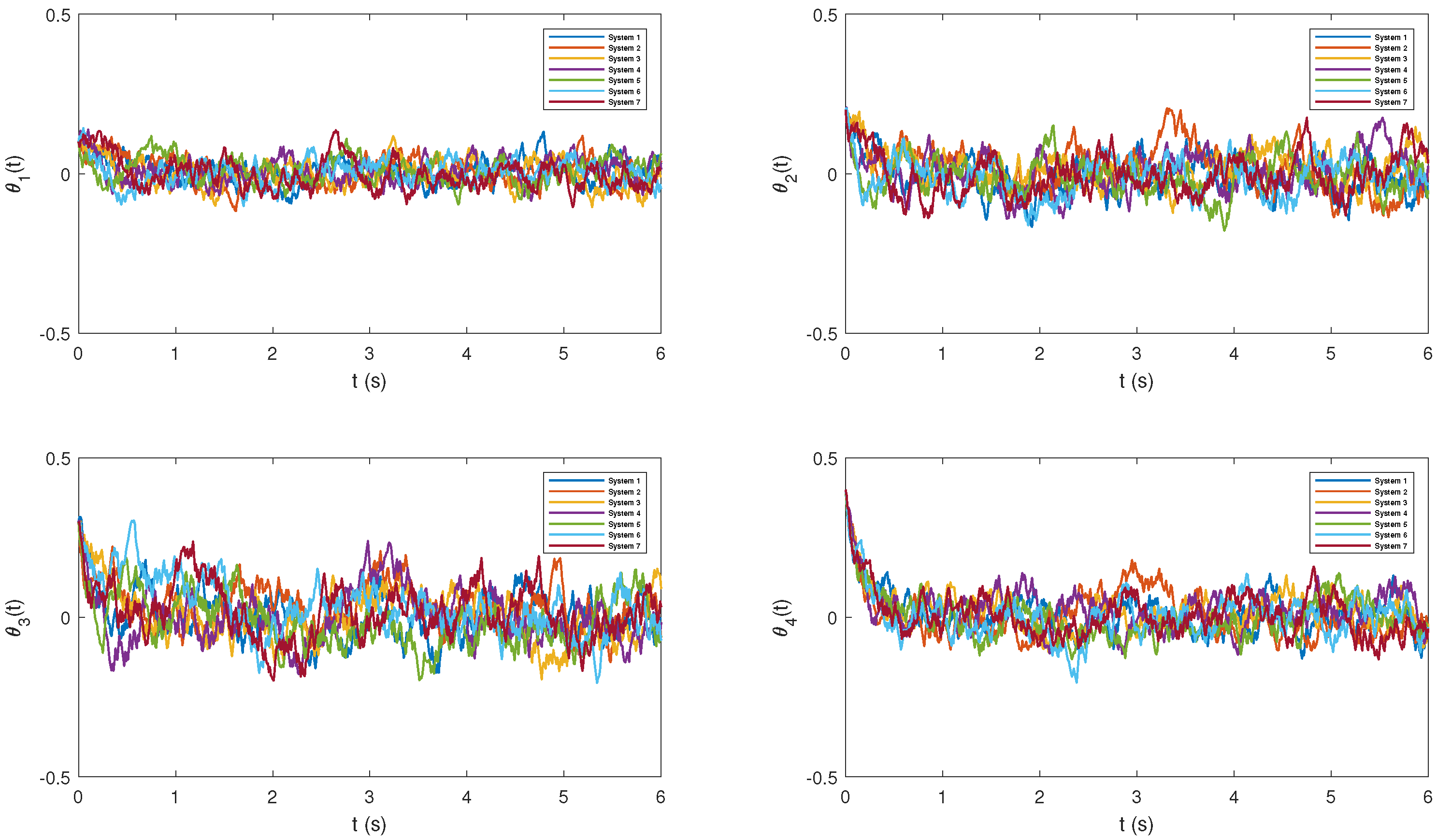
4. Numerical Test
5. Conclusions
Author Contributions
Funding
Data Availability Statement
Acknowledgments
Conflicts of Interest
References
- Kuramoto, Y. Self-entrainment of a population of coupled non-linear oscillators. In International Symposium on Mathematical Problems in Theoretical Physics, Kyoto, Japan, 23–29 January 1975; Springer: Berlin/Heidelberg, Germany, 1975; pp. 420–422. [Google Scholar]
- Nguyen, P.T.M.; Hayashi, Y.; Baptista, M.D.S.; Kondo, T. Collective almost synchronization-based model to extract and predict features of EEG signals. Sci. Rep. 2020, 10, 16342. [Google Scholar] [CrossRef] [PubMed]
- O´dor, G.; Kelling, J. Critical synchronization dynamics of the Kuramoto model on connectome and small world graphs. Sci. Rep. 2019, 9, 19621. [Google Scholar] [CrossRef] [PubMed]
- Gupta, S.; Zangrando, V.; Matijašević, L. Kuramoto model of coupled chemical oscillators: The effect of time-delay on synchronization. J. Chem. Phys. 2022, 157, 044108. [Google Scholar]
- Forrester, D.M. Arrays of coupled chemical oscillators. Sci. Rep. 2015, 5, 16994. [Google Scholar] [CrossRef] [PubMed]
- Guo, Y.; Zhang, D.; Li, Z.; Wang, Q.; Yu, D. Overviews on the applications of the Kuramoto model in modern power system analysis. Int. J. Electr. Power Energy Syst. 2021, 129, 106804. [Google Scholar] [CrossRef]
- Arinushkin, P.A.; Vadivasova, T.E. Nonlinear damping effects in a simplified power grid model based on coupled Kuramoto-like oscillators with inertia. Chaos Solitons Fractals 2021, 152, 111343. [Google Scholar] [CrossRef]
- Simpson-Porco, J.W. A theory of solvability for lossless power flow equations—Part II: Existence and uniqueness of high-voltage solutions. IEEE Trans. Control Netw. Syst. 2019, 6, 1117–1131. [Google Scholar]
- Naik, P.A.; Amer, M.; Ahmed, R.; Qureshi, S.; Huang, Z. Stability and bifurcation analysis of a discrete predator-prey system of Ricker type with refuge effect. Math. Biosci. Eng. 2024, 21, 4554–4586. [Google Scholar] [CrossRef]
- Naik, P.A.; Javaid, Y.; Ahmed, R.; Eskandari, Z.; Ganie, A.H. Stability and bifurcation analysis of a population dynamic model with Allee effect via piecewise constant argument method. J. Appl. Math. Comput. 2024, 70, 4189–4218. [Google Scholar] [CrossRef]
- West, D.B. Introduction to Graph Theory, 2nd ed.; Prentice Hall: Upper Saddle River, NJ, USA, 2001. [Google Scholar]
- Biggs, N.; Lloyd, E.K.; Wilson, R.J. Graph Theory, 1736–1936; Oxford University Press: Oxford, UK, 1986. [Google Scholar]
- Dragomir, S.S. Some Gronwall Type Inequalities and Applications; Nova Science: Hauppauge, NY, USA, 2003. [Google Scholar]
- Li, M.Y.; Shuai, Z. Global-stability problem for coupled systems of differential equations on networks. J. Differ. Equ. 2010, 248, 1–20. [Google Scholar] [CrossRef]
- Billingsley, P. Probability and Measure; John Wiley & Sons: Hoboken, NJ, USA, 2008. [Google Scholar]
- Krantz, S.G. Handbook of Complex Variables; Springer Science & Business Media: Berlin/Heidelberg, Germany, 1999. [Google Scholar]
- Mao, X. Stochastic Differential Equations and Applications; Elsevier: Amsterdam, The Netherlands, 2007. [Google Scholar]
- Zhang, J.; Zhu, J. Exponential synchronization of the high-dimensional Kuramoto model with identical oscillators under digraphs. Automatica 2019, 102, 122–128. [Google Scholar] [CrossRef]


Disclaimer/Publisher’s Note: The statements, opinions and data contained in all publications are solely those of the individual author(s) and contributor(s) and not of MDPI and/or the editor(s). MDPI and/or the editor(s) disclaim responsibility for any injury to people or property resulting from any ideas, methods, instructions or products referred to in the content. |
© 2024 by the authors. Licensee MDPI, Basel, Switzerland. This article is an open access article distributed under the terms and conditions of the Creative Commons Attribution (CC BY) license (https://creativecommons.org/licenses/by/4.0/).
Share and Cite
Tian, N.; Liu, X.; Kang, R.; Peng, C.; Li, J.; Gao, S. Noise-to-State Stability of Random Coupled Kuramoto Oscillators via Feedback Control. Mathematics 2024, 12, 3715. https://doi.org/10.3390/math12233715
Tian N, Liu X, Kang R, Peng C, Li J, Gao S. Noise-to-State Stability of Random Coupled Kuramoto Oscillators via Feedback Control. Mathematics. 2024; 12(23):3715. https://doi.org/10.3390/math12233715
Chicago/Turabian StyleTian, Ning, Xiaoqi Liu, Rui Kang, Cheng Peng, Jiaxi Li, and Shang Gao. 2024. "Noise-to-State Stability of Random Coupled Kuramoto Oscillators via Feedback Control" Mathematics 12, no. 23: 3715. https://doi.org/10.3390/math12233715
APA StyleTian, N., Liu, X., Kang, R., Peng, C., Li, J., & Gao, S. (2024). Noise-to-State Stability of Random Coupled Kuramoto Oscillators via Feedback Control. Mathematics, 12(23), 3715. https://doi.org/10.3390/math12233715