Article

Enhanced Carbon Price Forecasting Using Extended Sliding Window Decomposition with LSTM and SVR

1
School of Computer Science and Engineering, Macau University of Science and Technology, Macau 999078, China
2
Zhuhai-M.U.S.T. Science and Technology Research Institute, Zhuhai 519031, China
*
Author to whom correspondence should be addressed.
Mathematics 2024, 12(23), 3713; https://doi.org/10.3390/math12233713
Submission received: 22 September 2024 / Revised: 12 November 2024 / Accepted: 25 November 2024 / Published: 26 November 2024

Abstract

:
Accurately forecasting carbon prices plays a vital role in shaping environmental policies, guiding investment strategies, and accelerating the development of low-carbon technologies. However, traditional forecasting models often face challenges related to information leakage and boundary effects. This study proposes a novel extended sliding window decomposition (ESWD) mechanism to prevent information leakage and mitigate boundary effects, thereby enhancing decomposition quality. Additionally, a fully data-driven multivariate empirical mode decomposition (MEMD) technique is incorporated to further improve the model’s capabilities. Partial decomposition operations, combined with high-resolution and full-utilization strategies, ensure mode consistency. An empirical analysis of China’s largest carbon market, using eight key indicators from energy, macroeconomics, international markets, and climate fields, validates the proposed model’s effectiveness. Compared to traditional LSTM and SVR models, the hybrid model achieves performance improvements of 66.6% and 23.5% in RMSE for closing price prediction, and 73.8% and 10.8% for opening price prediction, respectively. Further integration of LSTM and SVR strategies enhances RMSE performance by an additional 82.7% and 8.3% for closing prices, and 30.4% and 4.5% for opening prices. The extended window setup (EW10) yields further gains, improving RMSE, MSE, and MAE by 11.5%, 35.4%, and 23.7% for closing prices, and 4.5%, 8.4%, and 4.2% for opening prices. These results underscore the significant advantages of the proposed model in enhancing carbon price prediction accuracy and trend prediction capabilities.

1. Introduction

Global warming, fueled by greenhouse gas emissions, threatens sustainable development, making emissions trading systems (ETSs) essential tools for climate mitigation [1,2,3]. The European Union’s ETS has led the way, and China, following its 2015 Paris Agreement commitments [4], launched a national carbon market in 2021 after successful pilot projects. By early 2021, China’s market covered over 20 industries and achieved substantial CO2 reductions, yet the path to its 2060 carbon neutrality goal remains challenging. Accurate carbon price forecasting is crucial, providing policymakers with insights for effective environmental strategies and guiding investors in sustainable projects [5]. Despite market complexities, advancing research in this field is vital to refine carbon pricing mechanisms and support global climate goals. However, the carbon market is a complex, nonlinear system influenced by various factors such as the economy, energy, financial markets, climate, and the environment, significantly increasing the difficulty of accurate predictions.
Current carbon price prediction methods include statistical models, artificial intelligence models, and decomposition–ensemble hybrid models. Traditional statistical economic models include autoregressive integrated moving average (ARIMA) models [6], vector autoregression (VAR) models [7], generalized autoregressive conditional heteroskedasticity (GARCH) models [8], and grey Markov models [9]. While these methods can achieve effective prediction results and provide a good theoretical basis grounded in statistical logic, they rely on linear assumptions and are primarily suitable for very short prediction spans, failing to fully capture the nonlinear characteristics hidden in time series data. To address this issue, artificial intelligence (AI) models have emerged and been applied to time series forecasting using data-driven approaches. These methods include artificial neural networks (ANNs) [10,11], support vector regression (SVR) [12], least squares support vector machines [13], extreme learning machines (ELMs) [14], and long short-term memory networks (LSTM) [15]. While AI models show promise, they often lack mechanisms to handle the instability and chaotic nature of carbon price series. For example, recent studies have explored the use of recurrent fuzzy neural networks (RFNNs) for chaotic time series [16] and combined Graph Convolutional Network (GCN) with Bidirectional Long Short-Term Memory (BiLSTM) to capture both spatial and temporal dependencies in economic data [17]. These advancements underscore the need for sophisticated AI models that can handle the complex dynamics of carbon prices, driving the development of hybrid and ensemble models that integrate multiple techniques to improve predictive accuracy.
Decomposition–ensemble hybrid models enhance robustness and accuracy by using decomposition techniques to capture the multi-scale information embedded in time series data. In this framework, the carbon price is decomposed into several simpler sub-signals, each of which is modeled independently. The final forecast is obtained by combining the predictions of these individual models. This approach effectively transforms the complex carbon price prediction task into a set of more manageable tasks, leading to improved overall prediction accuracy. A variety of decomposition techniques have been widely applied in decomposition–ensemble models. These include methods such as wavelet transform and variational mode decomposition (VMD) [18,19], which require researchers to select specific parameters in advance. For instance, wavelet transform necessitates the choice of a wavelet mother function, while VMD requires defining the number of decomposition layers. These requirements demand a certain level of expertise and familiarity with the data, adding complexity to their use. In contrast, empirical mode decomposition (EMD) [20] and its extensions, including ensemble empirical mode decomposition (EEMD) [21] and complete ensemble empirical mode decomposition with adaptive noise (CEEMDAN) [22], have gained significant attention due to their ability to adaptively decompose data without needing prior knowledge.
Cui et al. [23] combined EMD with PSO-SVM to improve carbon price prediction accuracy. Sun et al. [21] proposed a carbon price prediction model using EEMD and wavelet least squares support vector machine (wLSSVM), achieving higher prediction accuracy compared to single models. Yun et al. [24] introduced a hybrid model using CEEMDAN and LSTM to forecast carbon prices. Model validation using the settlement prices of European Union Allowance (EUA) products demonstrated significant improvements in prediction performance. Zhang et al. [25] applied EMD to decompose the original data and used ARIMA and LSSVM to predict different decomposed components, achieving better results than single models. Similarly, other researchers have found that using different prediction methods for different frequency components in decomposition–ensemble models can further improve prediction performance compared to using a single predictor [26,27,28,29].
Traditionally, the complete decomposition (CD) approach has been widely used, where the entire carbon price series is first decomposed and then split into training and testing sets. However, recent studies have raised concerns about potential information leakage with this method [30,31,32,33,34]. Specifically, during the CD process, future information from the test set may unintentionally be incorporated into the model during training, which relies on data that should not be accessible. This makes the CD method impractical for real-world applications, where future information is inherently unknown. To address this issue, researchers have employed a strategy called rolling decomposition (RD), which focuses on decomposing only the available data within the boundaries of known information during rolling forecasting [35,36,37].
However, the boundary effects that are commonly present in decomposition techniques can degrade the quality of the decomposed data as illustrated in Figure 1, ultimately reducing the predictive accuracy of decomposition–ensemble models. To address these challenges, this paper proposes a novel extended sliding decomposition strategy (ESWD) to prevent information leakage and improve the quality of data decomposition. Specifically, sliding decomposition is applied after the entire dataset has been divided into training and testing sets, ensuring that decomposition is performed exclusively on known information. For EMD and its extended techniques, boundary effects occur due to the lack of information outside the decomposition window, leading to uncertainty in determining the nature of extrema during cubic spline interpolation. In time series forecasting tasks, the data on the right side of the window represent future information, which is unknown and what the model is intended to predict. Since this future information is not available, boundary effects from the right side cannot be avoided. In contrast, the left side of the window contains known historical data. This allows us to suppress boundary effects on the left by extending the window to include more historical information, which provides a more accurate context for the decomposition. Our sliding decomposition strategy utilizes this extended window on the left to reduce left-side boundary effects, thereby improving the quality of data decomposition and enhancing the model’s prediction accuracy.
Additionally, most existing decomposition–ensemble models use univariate decomposition techniques. For multivariate data, this approach decomposes the univariate matrices one by one, potentially disrupting their intrinsic relationships and leading to biased results [38,39]. In contrast, multivariate empirical mode decomposition (MEMD) treats all variables as a unified system during the decomposition process. It analyzes the shared frequency distributions across all variables and extracts common frequencies in descending order from high to low. By doing so, MEMD preserves the multi-scale relationships between the target variable and its related variables more effectively, allowing for a deeper understanding of their interconnected dynamics. Using the MEMD method helps describe and interpret the driving factors of carbon prices at each time scale, thereby understanding their multi-scale driving processes and associated implications. Based on the above analysis, this paper proposes a new hybrid model for carbon price prediction. The model integrates MEMD, ESWD strategy, LSTM, and SVR. Its innovations and contributions include the following:
  • An ESWD strategy is proposed to address information leakage in carbon price forecasting. By incorporating an extended window on the left side, left-side boundary effects are mitigated, which enhances data decomposition quality.
  • Multivariate empirical mode decomposition (MEMD) is utilized for preprocessing multivariate data, which reduces prediction bias by preserving the intrinsic relationships between variables. Issues with inconsistent modal quantities are addressed through partial decomposition techniques.
  • A hybrid framework integrating MEMD and ESWD with SVR and LSTM models is developed to capture multi-scale features in carbon price data.
The remainder of this paper is structured as follows. Section 2 introduces the algorithms involved. Section 3 details the extended sliding window decomposition mechanism and the process of the proposed carbon price forecasting model. Section 4 describes the data used in the study, experimental setup and metrics, and the discussion of results, and the last section concludes the whole research work.

2. Methodology

2.1. Multivariate Empirical Mode Decomposition (MEMD)

The method of multivariate empirical mode decomposition (MEMD), proposed by Rehman and Mandic [40], serves as a multivariate extension of the EMD. It identifies common scales within multiple time series datasets and decomposes the signals into a similar number of intrinsic mode functions (IMFs) for each dataset. Multiple inputs are projected along different directions in an m-dimensional space. Let E ( t ) = e 1 ( t ) , e 2 ( t ) , , e m ( t ) denote the m data vectors as a function of time t, and let D θ k = d 1 k , d 2 k , , d m k denote the direction vector given by the angles θ k = θ 1 k , θ 2 k , , θ m 1 k in a direction set D where k = 1 , 2 , , N and N is the total number of directions. The IMFs of the m datasets can be obtained by the following algorithm:
(1) Create a set of suitable direction vectors by sampling from a unit hypersphere with ( m 1 ) dimensions.
(2) Calculate the projection P k θ ( t ) of the datasets E ( t ) along the direction vector D θ k for all k.
(3) Identify the temporal instants t i θ k corresponding to the maxima of the projection for all k.
(4) Interpolate t i θ k , E ( t i θ k ) to obtain the multivariate envelope curves e k θ ( t ) for all k.
(5) Calculate the mean of the envelope curves ( M ( t ) ) using M ( t ) = 1 N k = 1 N e θ k ( t ) .
(6) Extract the “detail” V ( t ) using V ( t ) = E ( t ) M ( t ) . If V ( t ) meets the stoppage criterion for a multivariate IMF, apply the aforementioned procedure to E ( t ) V ( t ) ; otherwise, apply it to V ( t ) .

2.2. Support Vector Regressions (SVR)

For data { x i , y i } i = 1 n , SVR can be described as a minimization problem:
minimize R = C to i = 1 n ( η i + η i * ) + 1 2 w T w
subject to y i w T φ ( x i ) b ε + η i y i + w T φ ( x i ) + b ε + η i * η i , η i * 0 , i = 1 , 2 , , n
where w represents the weight vector controlling the smoothness, b denotes the bias parameter, φ ( · ) is a nonlinear mapping function from the input space to the feature space, C to is a scalar parameter penalizing the extent of slack, η i and η i * denote two non-negative slack variables, and ε represents the tolerable error. By introducing Lagrange multipliers and optimality conditions, the problem described in Equations (1) and (2) can be transformed into a Lagrangian function. This function can be solved by maximizing its dual problem. The final solution for the weight vector w in Equations (1) and (2) is obtained in Equation (3).
w = i = 1 N ( μ i μ i * ) φ ( x i )
where μ i and μ i * , which satisfy the condition μ i μ i * = 0 , are the Lagrangian multipliers. Finally, based on Equation (3) and the use of the kernel function, the decision function is formulated as
f ( x ) = i = 1 N ( μ i μ i * ) Π ( x i , x j ) + b
where the kernel function Π ( x i , x j ) = φ T ( x i ) φ ( x j ) satisfies Mercer’s condition. The kernel function allows us to compute the mapping φ ( x ) implicitly, handling feature spaces of arbitrary dimensionality. The most common kernel functions include the polynomial kernel and the radial basis function (RBF). Each kernel has its parameters. Generally, among these kernel functions, the RBF kernel, given by Equation (5), is usually the preferred choice for constructing the SVR model because the RBF generally produces good results [41].
Π ( x i , x j ) = exp ( v x i x j 2 )
where v represents the kernel parameter.

2.3. Long Short-Term Memory Network (LSTM)

Long short-term memory (LSTM) networks are a specialized form of recurrent neural networks (RNNs) [42]. The primary motivation for the development of LSTMs was to address the issue of long-term dependencies in traditional RNNs, which often struggle to retain important information from distant points in time within a sequence. The LSTM architecture incorporates three pivotal gating mechanisms—an input gate, a forget gate, and an output gate—that collectively mitigate the problem of long-term dependencies, thereby enabling the network to capture and utilize information across extended temporal distances effectively.
The cell structure of LSTM is illustrated in Figure 2. The forget gate f t decides which information from the previous state unit S t 1 should be retained. It takes the previous output h t 1 and the current input x t , processes them through a sigmoid function and outputs a value between 0 and 1 to update the state unit S t . Similarly, the input gate g t determines which new information to store in the state unit. It filters h t 1 and x t through a sigmoid function to update the state unit S t . The output gate o t controls the information to be output from the state unit. It processes h t 1 and x t through a sigmoid function, and the state unit S t is then multiplied by o t after being processed by a tanh function to produce the output h t of the LSTM cell.
f t = σ ( b f + U f x t + W f h t 1 )
S t = f t S t 1 + g t σ ( b + U x t + W h t 1 )
g t = σ ( b g + U g x t + W g h t 1 )
o t = σ ( b o + U o x t + W o h t 1 )
h t = tanh ( S t ) o t
where f t , i t , o t , h t 1 , x t , and S t represent the forget gate, input gate, output gate, previous hidden state, current input, and current cell state, respectively. b, U, and W are the biases and weights associated with x t and h t 1 . σ denotes the sigmoid function, and tanh denotes the hyperbolic tangent function.

3. The Proposed Model

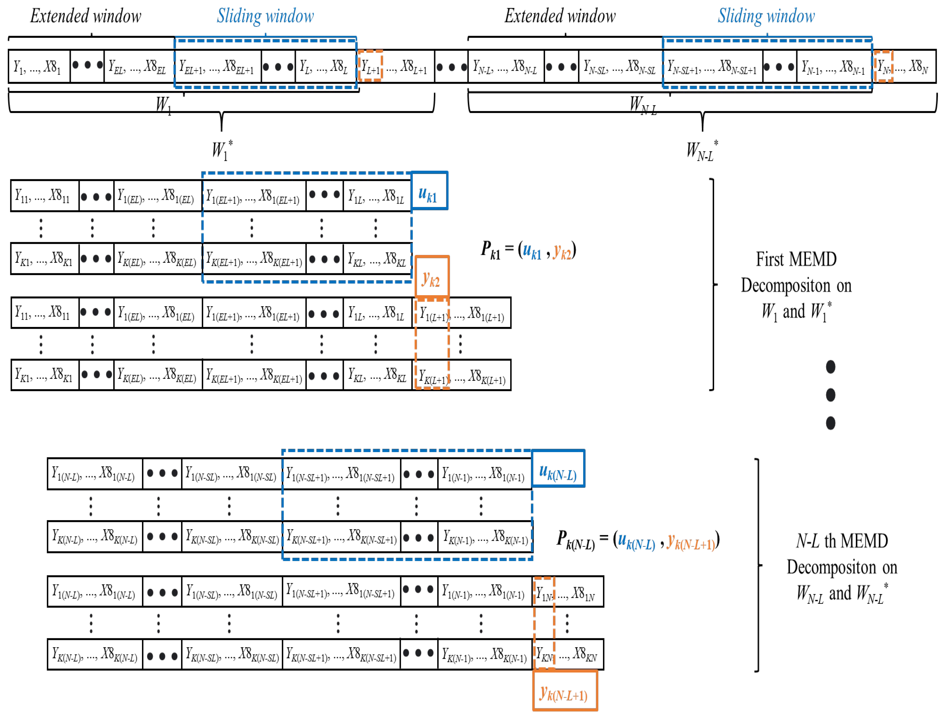
3.1. Extended Sliding Window Decomposition (ESWD) Mechanism

This paper introduces an extended sliding window decomposition (ESWD) mechanism, which aims to enhance the quality of data decomposition while mitigating the risk of information leakage in carbon price forecasting. The specific procedure is as follows: Initially, a window of length L is established to perform sliding segmentation on the multivariate time series, thereby generating a sequence of contiguous windows. Each window sequence W i encompasses carbon price and other variable data from time point i to i + L 1 , denoted as W i = { Y i , , X 8 i , , Y i + L 1 , , X 8 i + L 1 } . When forecasting the carbon price Y N on the N-th day, the ( N L ) -th window sequence W N L is selected and decomposed into K subsequences. This decomposition method, as illustrated in Figure 3, ensures that each subsequence contains only historical information, thereby eliminating the risk of data leakage.
To further suppress the boundary effect, we add an extended window to the sliding decomposition process. According to related research [43], the boundary effect typically stems from the uncertainty of values outside the window sequence edges. In time series forecasting tasks, future information on the right side of the window is unknown, while the historical information on the left side is known and can be utilized to improve the decomposition results [30]. Therefore, we construct a “real” window by merging the extended window (EW) and the sliding window (SW) for sliding decomposition, thereby improving the decomposition quality of the sliding window. Through this method, we obtain a series of window data for decomposition: { u k ( N L ) } = { u 1 ( N L ) , u 2 ( N L ) , , u K ( N L ) } , k [ 1 , K ] . Next, we decompose the window sequence W N L * that includes the data of the prediction day to obtain the multi-scale labels for the carbon price on the N-th day: { y k ( N L + 1 ) } = { Y 1 N , Y 2 N , , Y K N } . In this way, we can construct sample pairs for machine learning model training: P k ( N L ) = u k ( N L ) , y k ( N L + 1 ) .

3.2. Mode Number Selection Strategy

MEMD is a data-driven technique that adaptively decomposes data into subsequences, known as intrinsic mode functions (IMFs), based on the underlying frequency characteristics of the data. However, during the sliding window decomposition process, the frequency characteristics within each window can vary, resulting in different numbers of IMFs across windows. This variation leads to inconsistencies in the dimensionality of the resulting subsequences, u m k t , which creates challenges for predictive models that rely on uniform input dimensions. These inconsistencies can complicate the training and prediction processes, making it difficult to achieve accurate and efficient model performance.
To address this challenge, this paper introduces a partial decomposition strategy [30] that maintains a consistent number of modes across sliding windows by setting a minimum mode threshold. MEMD can adaptively decompose the original carbon price data into IMFs arranged sequentially from high to low frequencies, which enables the model to capture distinct frequency components and improve prediction accuracy. However, MEMD’s ability to vary the number of IMFs can lead to dimensional inconsistencies. For single-step prediction, high-frequency components are particularly important as they capture short-term fluctuations in carbon price, while low-frequency components are more stable and easier to predict. Therefore, we define a minimum number of components, K, during the sliding window decomposition process. By setting this threshold, we ensure that only the first K components are decomposed, with any remaining information aggregated into a residual component. This approach, known as partial decomposition, retains the lower-frequency content within the residual rather than decomposing it further, ensuring consistent input dimensions and enhancing model performance.
Based on this partial decomposition strategy, we propose two mode number selection strategies: the high-resolution strategy and the full-utilization strategy. These strategies define how the minimum mode number K is selected to balance multi-scale resolution with information retention:
  • High-resolution strategy: This strategy maintains a higher multi-scale resolution by discarding decomposition results that produce fewer than K modes. For example, if the minimum mode number standard is set to 6, then only windows that produce at least six IMFs are retained, with fewer-mode windows excluded from the model. This helps preserve finer details by focusing on windows with richer frequency content.
  • Full-utilization strategy: This strategy accepts a lower minimum mode number to maximize the use of available data, even if it means a slight reduction in multi-scale resolution. For example, if K = 5 , all windows with at least five IMFs are included. This strategy sacrifices some high-resolution detail but fully utilizes the information from all windows.
To illustrate these strategies, consider a sliding window decomposition distribution as follows: { ( 9 IMFs : 6 ) , ( 8 IMFs : 52 ) , ( 7 IMFs : 1078 ) , ( 6 IMFs : 634 ) , ( 5 IMFs : 1 ) } . Under the high-resolution strategy with K = 6 , only windows with at least six IMFs would be used, resulting in a higher degree of detail. In contrast, the full-utilization strategy with K = 5 would include all windows, potentially losing some finer detail but gaining more comprehensive data coverage.

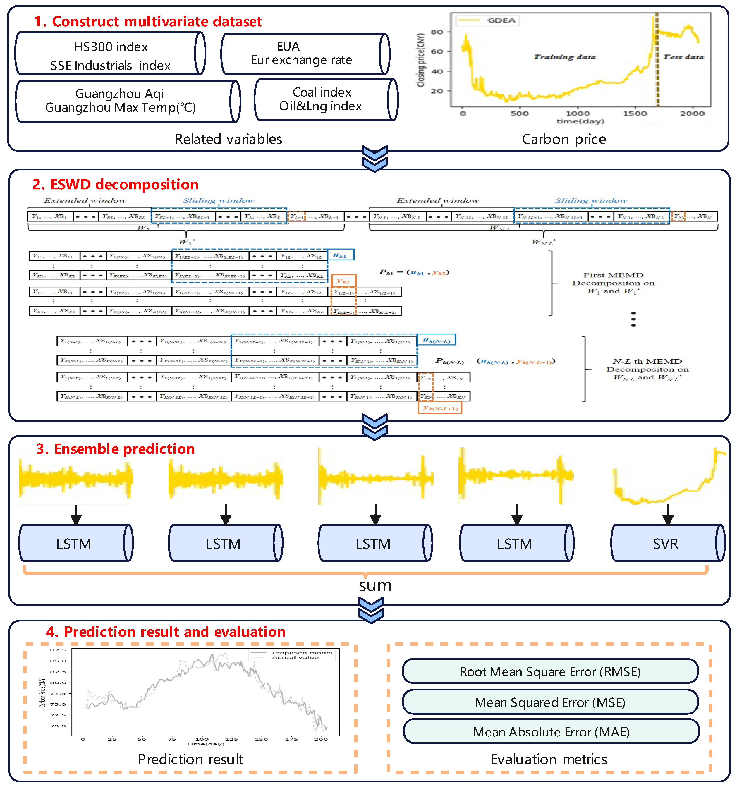
3.3. The Process of Carbon Price Forecasting

Ultimately, leveraging the aforementioned decomposition mechanism, a hybrid model for carbon price forecasting is constructed. This model is capable of synthesizing information from multiple subsequences and integrating learning outcomes to predict the carbon price in the subsequent phase. This process not only enhances the accuracy of predictions but also, by effectively utilizing historical data, mitigates the boundary effect, leading to more robust carbon price forecasting. The overall model flowchart is depicted in Figure 4, and the main steps are as follows:
1: Firstly, explore and analyze the factors influencing carbon trading prices, and then construct a dataset with series Y , X 1 , , X 8 .
2: Based on the extended sliding window technique, the original time series data are processed by slicing to generate a series of ordered window sequences, denoted as { W 1 , W 2 , , W N L } .
3: Decompose all window sequences and construct sample pairs P k ( N L ) = u k ( N L ) , y k ( N L + 1 ) based on the decomposition results, and then train the LSTM and SVR models.
4: Ultimately, apply the trained LSTM and SVR models to predict different subsequences. After the prediction is completed, aggregate the predicted results of these subsequences to obtain the final predicted value of the carbon price.

4. Case Studies

4.1. Study Object

The closing price of the daily carbon price of Guangzhou Carbon Emission Exchange is selected for the experiment. This exchange is a national platform and the sole non-free carbon emission quota trading platform designated by the Guangdong provincial government. It is also the only pilot in China to adopt paid allocation of carbon emission quotas. Thus, the Guangzhou carbon emission exchange is highly representative of China’s carbon emissions exchanges in terms of status and size. The data span from 14 March 2014 to 22 September 2023. As shown in Table 1, the multivariate dataset includes the target carbon price and eight additional influencing variables. Records with missing carbon price values were removed. For the experiments, the daily closing prices of carbon, energy, and macroeconomic indicators were used. The carbon price and additional variables series were divided into training, validation, and test sets in an 8:1:1 ratio as depicted in Figure 5. These sets were then segmented using a sliding window and decomposed with MEMD. Additionally, the samples were standardized to reduce noise influence. Additionally, Table 2 presents the target carbon price alongside eight influencing variables, summarizing key statistics—mean, max, min, standard deviation, and skewness—that capture the data’s variability and distribution.

4.2. Experimental Setup and Evaluation Metrics

When assessing the predictive accuracy of the model, we employed several commonly used statistical metrics, including root mean square error (RMSE), mean square error (MSE), mean absolute error (MAE), and directional accuracy (Dstat). The definitions of these metrics are as follows: where X i denotes the actual carbon price, Y i represents the predicted carbon price, and N is the number of samples. MSE measures the average of the squared differences between the predicted and actual values, while MAE is the mean of the absolute values of these differences. RMSE measures the magnitude of the average discrepancy between the predicted values of a statistical model and the actual values, making it suitable for continuous numerical forecasting problems. Dstat, on the other hand, measures the accuracy of direction prediction, indicating how often the model correctly predicts the up or down trend in carbon price. The lower the values of RMSE, MSE, and MAE, the higher the predictive accuracy of the model. A higher Dstat value indicates better accuracy in predicting the trend direction, which is especially valuable for decision-making in trading applications. The specific calculation methods for these evaluation metrics are as follows:
R M S E = 1 N i = 1 N X i Y i 2
M S E = 1 N i = 1 N X i Y i 2
M A E = 1 N i = 1 N X i Y i
D s t a t = 1 N 1 i = 1 N 1 1 , if ( X i + 1 X i ) ( Y i + 1 X i ) > 0 0 , otherwise × 100 %
In this study, the parameter settings and selection methods for the models used in the experiments are summarized in Table 3. We employ a grid search strategy to ascertain the hyperparameters of the SVR. Specifically, the GridSearchCV method is utilized to determine the kernel type, γ , and C. The GridSearchCV conducts an exhaustive search over a specified parameter grid. To elaborate, when employing the radial basis function (RBF) kernel, the candidates for γ are { 1 × 10 3 , 1 × 10 6 , 1 × 10 9 } , and the candidates for C are { 1 × 10 3 , 1 × 10 2 , 1 , 1 × 10 2 , 1 × 10 4 } . Conversely, when utilizing the linear kernel, only the C value is adjusted within the same range. For the setup of our LSTM network, we followed the recommendations from the literature [42]. The network is structured with two hidden layers and a batch size of 4, which is optimized for computational efficiency. The time step is configured to align with the size of the sliding window, enabling the model to use data from 60 trading days as input to predict the closing price of the next trading day. The input layer is designed with a dimension of 9, encompassing one target variable for forecasting and eight variables that represent influential factors. The experiments are implemented on the PyTorch platform, utilizing an Intel(R) Core(TM) i7-9750H CPU @ 2.60GHz and an NVIDIA GeForce GTX 1650 GPU for network training. The ADAM optimizer is employed with a batch size of B = 200 .

4.3. Discussion of Results

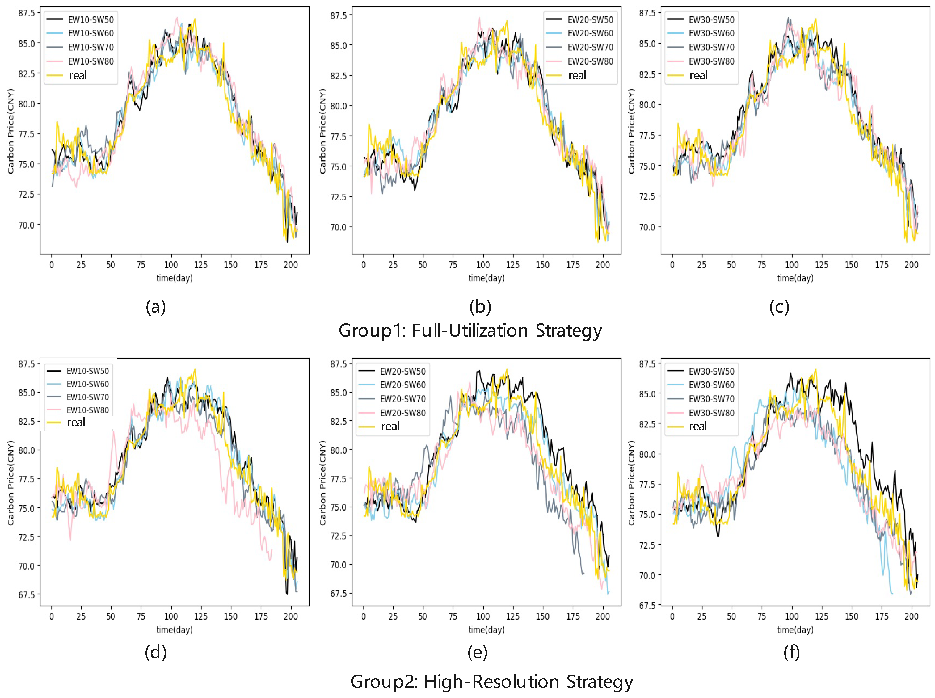
4.3.1. Expanded and Sliding Window Length Analysis

Before applying the ESWD mechanism, it is essential to determine an appropriate sliding window length. This parameter dictates the number of historical time steps considered when forecasting future carbon prices. To select a reasonable window length, we conducted a comprehensive analysis based on the autocorrelation of the carbon price series and its cross-correlation with other variables. In typical univariate time series forecasting, window size selection is primarily based on autocorrelation to capture relevant historical information. However, since our task involves multivariate forecasting, we extended this analysis to include cross-correlation between the target variable and related variables. This allows us to estimate an appropriate window range. Additionally, we refine the choice of window lengths by comparing the performance of different combinations on the validation set. While this selection is based on empirical observations, future work could aim to provide a more theoretical basis for determining optimal window length combinations.
As illustrated in Figure 6, the autocorrelation of the carbon price series diminishes with increasing time lags. However, for variables other than X6, X7, and X8, the cross-correlation with carbon prices increases with time lags. This indicates that selecting an appropriate window length is essential for capturing the relevance of carbon price fluctuations. A window that is too short may fail to fully leverage the available information, while a window that is too long could lead to excessive model complexity. Similarly, the length of the expansion window significantly impacts the quality of data decomposition and the complexity of the model. An expansion window that is too small might not adequately mitigate boundary effects, thereby affecting the quality of data and the model’s predictive performance. Conversely, an overly large expansion window could introduce redundant historical information, thereby increasing the model’s complexity. To strike a balance, we must explore suitable lengths for both the expansion and sliding windows in our experiments to ensure that we do not omit significant historical information while also avoiding overly complex models.

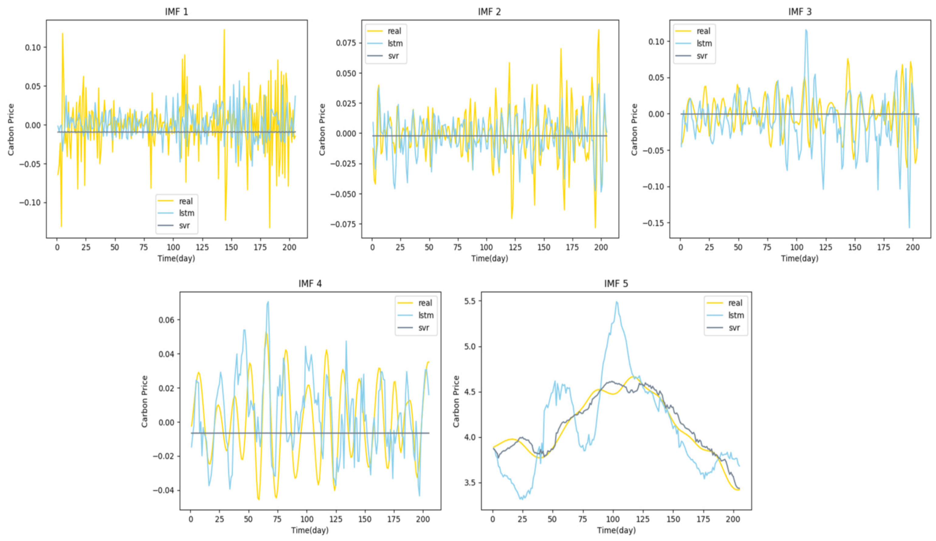
4.3.2. Decomposition Comparative Analysis

Following the parameter analysis of the ESWD mechanism, we proceeded to the validation phase, aimed at precisely assessing the specific impact of these parameters on model performance. Specifically, we meticulously adjusted the length of the sliding window, setting it to { 50 , 60 , 70 , 80 } , a range based on prior analysis intended to encompass key historical information that could be captured. Concurrently, the length of the expansion window was carefully selected as { 10 , 20 , 30 } to balance the suppression of boundary effects and model complexity. Subsequently, we performed the ESWD decomposition based on two-mode number selection strategies and compared the model’s performance under different settings.
In our study, we employed two mode number selection strategies to address the potential inconsistency. Table 4 provides a detailed account of the application outcomes of these strategies under various combinations of expansion and sliding windows. Specifically, when the extended window (EW) is set to 10 and the sliding window (SW) to 60, Figure 7 visually presents the distinct performance of these strategies in signal decomposition. As illustrated in Figure 7, “Y” represents the original carbon price time series, while “X1” to “X8” denote the time series of eight different factors influencing the carbon price. Through MEMD decomposition, we extracted mode components with similar frequencies from each series, labeled in descending order as “IMF 1” to “IMF 6”. Notably, compared to the original series, these mode components exhibit greater stability and regularity, laying a foundation for the construction of effective predictive models.
In Figure 7a,b, the first four mode components (“IMF 1” to “IMF 4”) are consistent across both strategies. However, the two strategies diverge in their treatment of the remaining mode components. Specifically, in Figure 7b, “IMF 5” is a composite of the low-frequency component “IMF 5” from Figure 7a and the residual component “IMF 6”. This discrepancy highlights the fundamental differences between the two strategies: the high-resolution strategy tends to decompose the signal into a greater number of components, potentially at the expense of some training data, whereas the full-utilization strategy prioritizes the integration of all available information, even if this leads to a reduction in the number of modal components.

4.3.3. Model Configuration Impact Analysis

In this study, we conducted an in-depth analysis of the predictive performance of the MEMD-ESWD-LSTM-SVR model under various window sizes and mode number selection strategies. As depicted in Figure 8, we observed that as the sliding window size increases, the performance initially improves to a peak and then gradually declines. For instance, with an extended window size of 10, the performance is optimal at SW-60, and it decreases at SW-70 and SW-80. This suggests that appropriately increasing the expansion window size can enhance model performance to a certain extent, but there exists an optimal range for the window size. This section is meant to offer a clearer illustration of the influence of window length and expansion window length on model performance, rather than serving as the basis for parameter selection.
The detailed metric evaluation results are summarized in Table 5. The study reveals that under the high-resolution strategy, when the sliding window size is set to 60 and the extended window size is 10, the model achieves the best values for most metrics, specifically RMSE, MSE, and MAE, with values of 2.567, 6.574, and 2.029, respectively. This finding indicates that this particular window configuration is most effective under the high-resolution strategy. Further analysis shows that under the same window configuration, the full-utilization strategy surpasses the high-resolution strategy in performance metrics, achieving an even lower RMSE of 2.469, MSE of 5.976, and MAE of 1.858, demonstrating a clear advantage of the full-utilization strategy for this specific configuration. In conclusion, selecting the appropriate sliding window length is crucial for optimizing model performance. Moreover, the full-utilization strategy provides higher predictive accuracy under specific window configurations, highlighting the need to consider the strategy’s specific impact on model performance when choosing a modal quantity selection strategy.

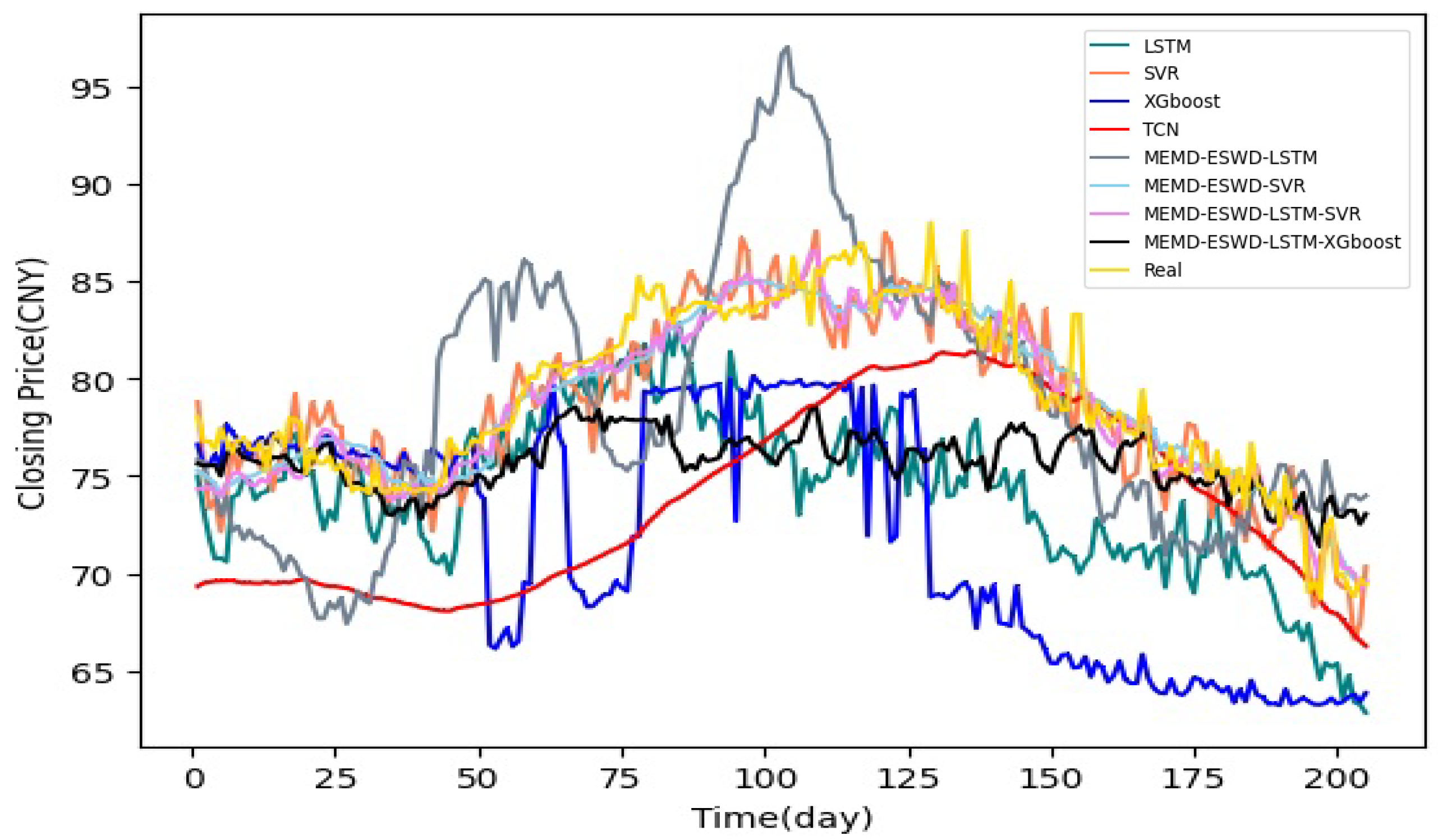
4.3.4. Prediction Performance Evaluation and Analysis

As mentioned in Section 1, research has shown that adopting differentiated predictive methods for components of different frequencies can yield superior forecasting results compared to using a single predictor [25,26,27,28,29]. Building upon this insight, we selected the LSTM and SVR models, both of which are widely used in time series forecasting. To evaluate the relative strengths of LSTM and SVR in predicting the different IMFs on a validation set, we conducted predictions for IMF1 through IMF5, with the results presented in Figure 9.
Our analysis reveals that SVR excels in capturing data trends, particularly demonstrating strong generalization capabilities when handling small-scale and high-dimensional data samples. However, its performance in capturing short-term fluctuations and high-frequency changes is somewhat limited. In contrast, the LSTM model is well suited for identifying and predicting short-term fluctuations and high-frequency components, although it may not be as smooth as SVR when fitting long-term trends. This differentiation highlights the rationale behind Figure 8, which visually underscores the complementary roles of SVR and LSTM in handling frequency-specific IMF predictions.
Therefore, to effectively combine the strengths of both models, the MEMD-ESWD-LSTM-SVR carbon price forecasting model proposed in this paper adopts the following strategy: high-frequency components are assigned to LSTM for prediction, while low-frequency and trend components are allocated to SVR. Through this integrated approach, we can more comprehensively predict the characteristics of different IMFs, achieving superior forecasting performance. In this study, we conducted a comprehensive evaluation of the performance of various models on the daily carbon price forecasting task. Initially, we employed single artificial intelligence models, including SVR and LSTM. Furthermore, in the hybrid models, we compared the performance of the MEMD-ESWD-LSTM model and the MEMD-ESWD-SVR model to assess their relative advantages compared to the proposed MEMD-ESWD-LSTM-SVR model. Concurrently, based on the discussion results in Section 4.3.3, we also selected two sets of window combinations (EW = 10 and SW = 50, and EW = 10 and SW = 60) for experiments with the decomposition ensemble forecasting model. The experiments for the single prediction models were based on sliding window sizes of 50 and 60. Figure 10 displays the specific predictive performance of these models. It was observed that the predictive performance of LSTM and MEMD-ESWD-LSTM was relatively poor, with significant deviations from the actual values. In contrast, the hybrid models that incorporated decomposition techniques, MEMD-ESWD-SVR and MEMD-ESWD-LSTM-SVR, demonstrated superior performance, with their forecast curves closely tracking the actual values.
A comprehensive comparison of model performance metrics is provided in Table 6, illustrating the comparative effectiveness of various approaches for both closing and opening price forecasts. The results suggest that, due to the multi-scale characteristics of the time series, single models generally perform less effectively than hybrid models. Specifically, the SVR model demonstrated stable predictive capabilities, particularly in capturing trend components of the series. In contrast, the predictive performance of the LSTM model exhibited greater variability, potentially due to the limited sample size, which may have hindered adequate training. In the case of hybrid models, all configurations—except those utilizing LSTM as the sole predictor—achieved superior predictive accuracy compared to single models. Notably, the MEMD-ESWD-LSTM-SVR hybrid model, which leverages the complementary strengths of LSTM and SVR, yielded the best overall performance across both closing and opening price predictions. With the EW10-SW60 window configuration, this model achieved RMSE, MSE, and MAE values of 1.503, 2.259, and 1.165 for closing prices and 1.601, 2.562, and 1.306 for opening prices, outperforming all other configurations (see Figure 11 and Table 7).
Compared to the best-performing single LSTM and SVR models, the proposed hybrid model showed RMSE improvements of 66.6% and 23.5% for closing prices and 73.8% and 10.8% for opening prices, respectively. Furthermore, in comparison with the MEMD-ESWD-LSTM and MEMD-ESWD-SVR models individually, the hybrid approach combining these two models achieved additional RMSE improvements of 82.7% over MEMD-ESWD-LSTM and 8.3% over MEMD-ESWD-SVR in the closing price prediction task, and 30.4% and 4.5%, respectively, for opening price predictions. The introduction of the EW10 extended window configuration also contributed positively, enhancing RMSE, MSE, and MAE by 11.5%, 35.4%, and 23.7% on average for closing prices and by 4.5%, 8.4%, and 4.2% for opening prices, when compared to configurations without the extended window setting. While these findings underscore the utility of ESWD preprocessing and the combination of LSTM with SVR for improved forecasting accuracy, there remains scope for further refinement in predictive precision.
In addition to accuracy metrics, the proposed model demonstrated promising performance in directional accuracy, as measured by the Dstat indicator. Achieving Dstat values of 0.566 for closing prices and 0.595 for opening prices, the MEMD-ESWD-LSTM-SVR hybrid model effectively captured the trend direction of carbon price movements. Directional accuracy is particularly significant, as it provides actionable insights that can guide strategic decision-making in carbon price trading. A high Dstat value indicates the model’s potential to identify upward or downward price trends, which is especially valuable in real-world applications where the direction of price movement is often as critical as the predicted price level.
In summary, the proposed MEMD-ESWD-LSTM-SVR model demonstrated consistent improvements in both accuracy and directional reliability for carbon price forecasting, leveraging the strengths of hybrid modeling and an extended sliding window approach. Although the results indicate significant enhancements over single models, further improvements in predictive precision remain possible, offering potential avenues for future research.

5. Conclusions

This paper presents an innovative multivariate approach for carbon price forecasting, aiming to enhance the accuracy and adaptability of forecasting models through advanced decomposition techniques. Initially, an ESWD mechanism was designed to effectively prevent information leakage issues inherent in traditional CD methods and to mitigate the adverse impact of boundary effects on decomposition quality by introducing an extended window. Subsequently, a fully data-driven MEMD technique was employed to further enhance the model’s capabilities. To address the issue of inconsistent mode numbers in window decomposition, the study introduced partial decomposition operations and proposed two strategies—the high-resolution strategy and the full-utilization strategy—to ensure the consistency of modal numbers.
In the empirical analysis, the study selected the largest carbon market in China as a case study and combined eight representative indicators from the fields of energy, macroeconomics, international markets, and climate to verify the effectiveness of the proposed model. The results show that, compared to traditional LSTM and SVR models, the proposed hybrid model achieved performance improvements of 66.6% and 23.5% in the RMSE indicator for closing price prediction, and 73.8% and 10.8% for opening price prediction, respectively. Furthermore, by integrating strategies using both LSTM and SVR models, the performance in the RMSE indicator was further enhanced by 82.7% and 8.3% in closing price prediction, and 30.4% and 4.5% in opening price prediction, respectively. Additionally, the introduction of the EW-10 extended window setting contributed to further performance improvements, achieving average gains of 11.5%, 35.4%, and 23.7% in the RMSE, MSE, and MAE indicators for closing prices, and 4.5%, 8.4%, and 4.2% for opening prices, respectively.
Besides accuracy metrics, the proposed model showed a promising directional accuracy, as indicated by the Dstat indicator, achieving values of 56.6% for closing prices and 59.5% for opening prices. Directional accuracy is particularly important for providing actionable insights in carbon trading, where understanding price trends—whether upward or downward—is critical for effective decision-making. The high Dstat values achieved by the proposed model underscore its potential to capture directional patterns, which adds practical value for stakeholders in the carbon market. It is also worth noting that while the study has demonstrated the effectiveness of the decomposition methods, optimizing predictive accuracy was not the primary objective. Consequently, further refinement is possible to enhance predictive precision. Future work may focus on fine-tuning model parameters and exploring additional strategies to achieve the highest possible forecasting performance.
The model proposed in this study is particularly tailored to the nonlinear and non-stationary characteristics of carbon price time series by organically combining MEMD decomposition with LSTM and SVR. This method not only enhances the model’s adaptability to market fluctuations but also significantly improves the accuracy of predictions. Accurate carbon price forecasting is of great significance for enterprises to make informed decisions in production and operation, to avoid market risks, and to optimize resource allocation. At the same time, it also provides scientific decision support for policymakers, helping governments to formulate more reasonable environmental policies and emission reduction targets and to effectively address the challenges of climate change. Despite its advantages, the proposed method has certain limitations. First, the MEMD and ESWD processes, while effective, are computationally intensive, potentially affecting real-time forecasting capabilities when applied to large datasets or high-frequency data. Additionally, the accuracy of the model is sensitive to the selection of parameters such as the number of IMFs and the sliding window size, which may require fine-tuning for different datasets. Finally, although the extended window helps mitigate boundary effects, further research is needed to fully understand its impact across diverse data patterns. Addressing these challenges will be key to refining the model for broader applications and improving its computational efficiency.

Author Contributions

X.C.: Conceptualization, methodology, formal analysis, writing—original draft preparation, visualization, software. D.L.: supervision and reviewing, methodology, project administration, validation. L.F.: investigation, data curation, formal analysis, software, validation, visualization. All authors have read and agreed to the published version of the manuscript.

Funding

This research was funded by the National Key R&D Program of China No. 2019YFB1804400 and the Science and Technology Development Fund (FDCT) of Macau under Grant 0095/2023/RIA2.

Data Availability Statement

The data are available from the corresponding author on reasonable request.

Conflicts of Interest

The authors declare no conflicts of interest.

References

  1. Wara, M. Is the global carbon market working? Nature 2007, 445, 595–596. [Google Scholar] [CrossRef] [PubMed]
  2. Boyce, J.K. Carbon pricing: Effectiveness and equity. Ecol. Econ. 2018, 150, 52–61. [Google Scholar] [CrossRef]
  3. Farouq, I.S.; Sambo, N.U.; Ahmad, A.U.; Jakada, A.H.; Danmaraya, I. Does financial globalization uncertainty affect CO2 emissions? Empirical evidence from some selected SSA countries. Quant. Financ. Econ 2021, 5, 247–263. [Google Scholar] [CrossRef]
  4. Savaresi, A. The Paris Agreement: A new beginning? J. Energy Nat. Resour. Law 2016, 34, 16–26. [Google Scholar] [CrossRef]
  5. Narassimhan, E.; Gallagher, K.S.; Koester, S.; Alejo, J.R. Carbon pricing in practice: A review of existing emissions trading systems. Clim. Policy 2018, 18, 967–991. [Google Scholar] [CrossRef]
  6. Zhu, B.; Chevallier, J.; Zhu, B.; Chevallier, J. Carbon price forecasting with a hybrid Arima and least squares support vector machines methodology. In Pricing and Forecasting Carbon Markets: Models and Empirical Analyses; Springer: Berlin/Heidelberg, Germany, 2017; pp. 87–107. [Google Scholar]
  7. Zhu, B.; Wang, P.; Chevallier, J.; Wei, Y.M.; Xie, R. Enriching the VaR framework to EEMD with an application to the European carbon market. Int. J. Financ. Econ. 2018, 23, 315–328. [Google Scholar] [CrossRef]
  8. Paolella, M.S.; Taschini, L. An econometric analysis of emission allowance prices. J. Bank. Financ. 2008, 32, 2022–2032. [Google Scholar] [CrossRef]
  9. Segnon, M.; Lux, T.; Gupta, R. Modeling and forecasting the volatility of carbon dioxide emission allowance prices: A review and comparison of modern volatility models. Renew. Sustain. Energy Rev. 2017, 69, 692–704. [Google Scholar] [CrossRef]
  10. Tsai, M.T.; Kuo, Y.T. A forecasting system of carbon price in the carbon trading markets using artificial neural network. Int. J. Environ. Sci. Dev. 2013, 4, 163. [Google Scholar] [CrossRef]
  11. Zou, Y.; Lin, Z.; Li, D.; Liu, Z. Advancements in Artificial Neural Networks for health management of energy storage lithium-ion batteries: A comprehensive review. J. Energy Storage 2023, 73, 109069. [Google Scholar] [CrossRef]
  12. Zhu, B.; Ye, S.; Wang, P.; Chevallier, J.; Wei, Y.M. Forecasting carbon price using a multi-objective least squares support vector machine with mixture kernels. J. Forecast. 2022, 41, 100–117. [Google Scholar] [CrossRef]
  13. Cai, X.; Luo, S. Prediction of Spot Price of Iron Ore Based on PSR-WA-LSSVM Combined Model. J. Comput. Inf. Technol. 2021, 29, 27–38. [Google Scholar] [CrossRef]
  14. Xu, H.; Wang, M.; Jiang, S.; Yang, W. Carbon price forecasting with complex network and extreme learning machine. Phys. A Stat. Mech. Its Appl. 2020, 545, 122830. [Google Scholar] [CrossRef]
  15. Huang, Y.; Shen, L.; Liu, H. Grey relational analysis, principal component analysis and forecasting of carbon emissions based on long short-term memory in China. J. Clean. Prod. 2019, 209, 415–423. [Google Scholar] [CrossRef]
  16. Nasiri, H.; Ebadzadeh, M.M. MFRFNN: Multi-functional recurrent fuzzy neural network for chaotic time series prediction. Neurocomputing 2022, 507, 292–310. [Google Scholar] [CrossRef]
  17. Lazcano, A.; Herrera, P.J.; Monge, M. A combined model based on recurrent neural networks and graph convolutional networks for financial time series forecasting. Mathematics 2023, 11, 224. [Google Scholar] [CrossRef]
  18. Wang, J.; Cui, Q.; He, M. Hybrid intelligent framework for carbon price prediction using improved variational mode decomposition and optimal extreme learning machine. Chaos Solitons Fractals 2022, 156, 111783. [Google Scholar] [CrossRef]
  19. Nasiri, H.; Ebadzadeh, M.M. Multi-step-ahead stock price prediction using recurrent fuzzy neural network and variational mode decomposition. Appl. Soft Comput. 2023, 148, 110867. [Google Scholar] [CrossRef]
  20. Zhu, B.; Han, D.; Wang, P.; Wu, Z.; Zhang, T.; Wei, Y.M. Forecasting carbon price using empirical mode decomposition and evolutionary least squares support vector regression. Appl. Energy 2017, 191, 521–530. [Google Scholar] [CrossRef]
  21. Sun, W.; Xu, C. Carbon price prediction based on modified wavelet least square support vector machine. Sci. Total Environ. 2021, 754, 142052. [Google Scholar] [CrossRef]
  22. Cheng, M.; Xu, K.; Geng, G.; Liu, H.; Wang, H. Carbon price prediction based on advanced decomposition and long short-term memory hybrid model. J. Clean. Prod. 2024, 451, 142101. [Google Scholar] [CrossRef]
  23. Huan-ying, C.; Xiang-sheng, D. Carbon price forecasts in Chinese carbon trading market based on EMD-GA-BP and EMD-PSO-LSSVM. Oper. Res. Manag. Sci. 2018, 27, 133. [Google Scholar]
  24. Yun, P.; Huang, X.; Wu, Y.; Yang, X. Forecasting carbon dioxide emission price using a novel mode decomposition machine learning hybrid model of CEEMDAN-LSTM. Energy Sci. Eng. 2023, 11, 79–96. [Google Scholar] [CrossRef]
  25. Zhang, W.; Wu, Z. Optimal hybrid framework for carbon price forecasting using time series analysis and least squares support vector machine. J. Forecast. 2022, 41, 615–632. [Google Scholar] [CrossRef]
  26. Zhu, J.; Wu, P.; Chen, H.; Liu, J.; Zhou, L. Carbon price forecasting with variational mode decomposition and optimal combined model. Phys. A Stat. Mech. Its Appl. 2019, 519, 140–158. [Google Scholar] [CrossRef]
  27. Zhang, Y.J.; Zhang, J.L. Volatility forecasting of crude oil market: A new hybrid method. J. Forecast. 2018, 37, 781–789. [Google Scholar] [CrossRef]
  28. Zhu, B.; Yuan, L.; Ye, S. Examining the multi-timescales of European carbon market with grey relational analysis and empirical mode decomposition. Phys. A Stat. Mech. Its Appl. 2019, 517, 392–399. [Google Scholar] [CrossRef]
  29. Zhang, J.; Wei, Y.M.; Li, D.; Tan, Z.; Zhou, J. Short term electricity load forecasting using a hybrid model. Energy 2018, 158, 774–781. [Google Scholar] [CrossRef]
  30. Cai, X.; Li, D. M-EDEM: A MNN-based Empirical Decomposition Ensemble Method for improved time series forecasting. Knowl.-Based Syst. 2024, 283, 111157. [Google Scholar] [CrossRef]
  31. Wu, F.; Li, D.; Zhao, J.; Jiang, H.; Luo, X. SDIPPWV: A novel hybrid prediction model based on stepwise decomposition-integration-prediction avoids future information leakage to predict precipitable water vapor from GNSS observations. Sci. Total Environ. 2024, 933, 173116. [Google Scholar] [CrossRef]
  32. Liu, T.; Ma, X.; Li, S.; Li, X.; Zhang, C. A stock price prediction method based on meta-learning and variational mode decomposition. Knowl.-Based Syst. 2022, 252, 109324. [Google Scholar] [CrossRef]
  33. Huang, Y.; Deng, Y. A new crude oil price forecasting model based on variational mode decomposition. Knowl.-Based Syst. 2021, 213, 106669. [Google Scholar] [CrossRef]
  34. He, M.; Wu, S.f.; Kang, C.x.; Xu, X.; Liu, X.f.; Tang, M.; Huang, B.b. Can sampling techniques improve the performance of decomposition-based hydrological prediction models? Exploration of some comparative experiments. Appl. Water Sci. 2022, 12, 175. [Google Scholar] [CrossRef]
  35. Yu, L.; Ma, Y.; Ma, M. An effective rolling decomposition-ensemble model for gasoline consumption forecasting. Energy 2021, 222, 119869. [Google Scholar] [CrossRef]
  36. Quilty, J.; Adamowski, J. Addressing the incorrect usage of wavelet-based hydrological and water resources forecasting models for real-world applications with best practices and a new forecasting framework. J. Hydrol. 2018, 563, 336–353. [Google Scholar] [CrossRef]
  37. Liu, Y.; Huang, S.; Tian, X.; Zhang, F.; Zhao, F.; Zhang, C. A stock series prediction model based on variational mode decomposition and dual-channel attention network. Expert Syst. Appl. 2024, 238, 121708. [Google Scholar] [CrossRef]
  38. He, K.; Zha, R.; Wu, J.; Lai, K.K. Multivariate EMD-based modeling and forecasting of crude oil price. Sustainability 2016, 8, 387. [Google Scholar] [CrossRef]
  39. Ghazani, M.M. Analyzing the drivers of CO2 allowance prices in EU ETS under the COVID-19 pandemic: Considering MEMD approach with a novel filtering procedure. J. Clean. Prod. 2023, 427, 139043. [Google Scholar]
  40. Rehman, N.; Mandic, D.P. Multivariate empirical mode decomposition. Proc. R. Soc. A Math. Phys. Eng. Sci. 2010, 466, 1291–1302. [Google Scholar] [CrossRef]
  41. Fan, G.F.; Peng, L.L.; Hong, W.C.; Sun, F. Electric load forecasting by the SVR model with differential empirical mode decomposition and auto regression. Neurocomputing 2016, 173, 958–970. [Google Scholar] [CrossRef]
  42. Hochreiter, S.; Schmidhuber, J. Long short-term memory. Neural Comput. 1997, 9, 1735–1780. [Google Scholar] [CrossRef]
  43. Huang, N.E.; Shen, Z.; Long, S.R.; Wu, M.C.; Shih, H.H.; Zheng, Q.; Yen, N.C.; Tung, C.C.; Liu, H.H. The empirical mode decomposition and the Hilbert spectrum for nonlinear and non-stationary time series analysis. Proc. R. Soc. London. Ser. A Math. Phys. Eng. Sci. 1998, 454, 903–995. [Google Scholar] [CrossRef]
Figure 1. Illustration of boundary effects. The red line shows the accurate decomposition outcome for the full signal A. In comparison, the green line represents the decomposition result obtained when future information from signal A is omitted, resulting in a noticeable discrepancy from the accurate outcome.
Mathematics 12 03713 g001
Figure 2. Architecture of LSTM unit.
Mathematics 12 03713 g002
Figure 3. Proposed extended sliding window decomposition mechanism. Two window sequences, W N L and W N L * , are rolling decomposed to construct the pairs P k ( N L ) = ( u k ( N L ) , y k ( N L + 1 ) ) .
Mathematics 12 03713 g003
Figure 4. Process of the proposed MEMD-ESWD-LSTM-SVR carbon price forecasting model.
Mathematics 12 03713 g004
Figure 5. Trends of daily carbon price and related variables over time (14 March 2014–22 September 2023).
Mathematics 12 03713 g005
Figure 6. Autocorrelation of carbon price series and correlation between other variables.
Mathematics 12 03713 g006
Figure 7. A simple example of different modal number selection strategies.
Mathematics 12 03713 g007
Figure 8. A comparative analysis of window configurations and modal number strategies on the performance of MEMD-ESWD-LSTM-SVR models. (ac) Performance under the Full-Utilization Strategy with extended window sizes from 10 to 30 and varying sliding window lengths. (df) Performance under the High-Resolution Strategy with the same settings.
Mathematics 12 03713 g008
Figure 9. Performance evaluation of LSTM and SVR on IMFs of carbon price.
Mathematics 12 03713 g009
Figure 10. Comparison of prediction performance of multiple models on the daily closing carbon price prediction task.
Mathematics 12 03713 g010
Figure 11. Comparison of prediction performance of multiple models on the daily opening carbon price prediction task.
Mathematics 12 03713 g011
Table 1. Overview of carbon prices and additional influencing variables.
VariableSymbolDescriptionReasons for Choosing Variables
GDEAYcarbon priceRegional carbon market allocates and trades quotas.
Coal indexX1energy priceRaw material prices impact energy producers and various sectors.
Oil&Lng indexX2energy price
HS300 indexX3macroeconomicsMacroeconomic changes reflect total social consumption and demand.
SSE Industrials indexX4macroeconomicsMacroeconomics affects carbon prices via industry and electricity, reflected by the SSE Industrials index.
EUAX5international marketImperfect pricing and trading affect international carbon market prices.
EUR exchange rateX6international marketUsed as a reference for pricing.
Guangzhou AqiX7climateAQI reflects greenhouse gas levels.
Guangzhou Max Temp (°C)X8climateTemperature affects residential and commercial energy consumption.
Table 2. Statistical characterization of data.
VariablesMaxMinMeanStdSkewness
Y35.4195.268.1024.450.91
X12749.695136.801587.81796.191.00
X22432.524415.321595.59462.320.75
X33801.725807.722086.97765.25−0.11
X42336.244837.491263.07524.680.88
X529.5597.673.9329.121.04
X67.588.586.490.41−0.14
X767.84205.0013.0030.461.17
X827.1238.006.006.35−0.62
Table 3. Parameter settings and selection methods for the models used in the experiments.
ModelsParameter Setting MethodParameter Setting and Search Range
SVRGrid SearchGrid search with RBF and linear kernels.
‘gamma’: [ 1 × 10 3 , 1 × 10 6 , 1 × 10 9 ],
‘C’: [0.001, 0.01, 1, 100, 10,000],
LSTMEmpirical settingLSTM layer with 60 units,
Optimized using SGD with momentum,
trained for 60 epochs.
XGboostEmpirical settingmaximum depth of 3,
learning rate η = 0.2
and 100 boosting rounds.
TCNEmpirical settingThree Conv1D layers with 128 filters,
kernel size 2, and increasing dilation rates (1, 2, 4).
Final fully connected layer for prediction.
Table 4. Results of modal number selection for different expanded and sliding window lengths.
Window LengthHigh-Resolution StrategyFull-Utilization Strategy
SW-50SW-60SW-70SW-80SW-50SW-60SW-70SW-80
EW-1066675556
EW-2066775566
EW-3067775666
Table 5. Model performance metrics for window configurations and modal number strategies.
Window
Length
MetricsHigh-Resolution StrategyFull-Utilization Strategy
SW-50SW-60SW-70SW-80SW-50SW-60SW-70SW-80
EW-10RMSE2.6652.5672.9343.4962.5182.4692.8853.178
MSE7.1716.5748.36711.9526.5745.9768.36710.160
MAE2.0782.0292.3712.8601.9561.8582.3962.567
EW-20RMSE3.3252.8113.0313.2022.7382.6162.9093.129
MSE11.3557.7698.96410.1607.7696.5748.3679.562
MAE2.5672.2252.4452.6162.1512.0782.2982.469
EW-30RMSE3.4222.8603.1053.5452.9342.7383.2023.276
MSE11.9528.3679.56212.5508.3677.76910.16010.757
MAE2.6402.3222.5912.9092.3222.2002.5912.665
Table 6. Comparison of closing price forecast results.
ModelsRMSEMSEMAEDstatTIME (s)
LSTM(SW60)4.49720.9763.34650.7%50.21
SVR(SW60)1.9653.8591.55153.6%22.43
XGboost(SW60)5.01825.1814.13551.1%1.13
TCN(SW60)6.89547.5456.56547.8%100.35
MEMD-ESWD-LSTM(EW10-SW60)8.99680.9297.43448.8%28,887.455
MEMD-ESWD-SVR(EW10-SW60)1.5372.3411.27953.2%50,264.21
MEMD-ESWD-LSTM-XGboost(EW10-SW60)4.89723.9763.74652.7%28,845.557
MEMD-ESWD-LSTM-SVR(EW10-SW60)1.5032.2591.16556.6%49,607.601
Table 7. Comparison of opening price forecast results.
ModelsRMSEMSEMAEDstatTIME (s)
LSTM(SW60)6.1245.2415.8250.6%30.786
SVR(SW60)1.7943.2171.43755.5%66.324
XGboost(SW60)4.89123.9213.76249.8%1.197
TCN(SW60)2.566.5562.23849.3%134.21
MEMD-ESWD-LSTM(EW10-SW60)7.30153.3086.40154.6%21,863.3
MEMD-ESWD-SVR(EW10-SW60)1.6772.8131.34854.1%49,881.365
MEMD-ESWD-LSTM-XGboost(EW10-SW60)3.43311.7882.7449.8%21,809.668
MEMD-ESWD-LSTM-SVR(EW10-SW60)1.6012.5621.30659.5%47,240.23
Disclaimer/Publisher’s Note: The statements, opinions and data contained in all publications are solely those of the individual author(s) and contributor(s) and not of MDPI and/or the editor(s). MDPI and/or the editor(s) disclaim responsibility for any injury to people or property resulting from any ideas, methods, instructions or products referred to in the content.

