Article

Approximation of Time-Frequency Shift Equivariant Maps by Neural Networks

Department of Mathematics and Big Data Science, Kumoh National Institute of Technology, Gumi 39177, Gyeongsangbuk-do, Republic of Korea
Mathematics 2024, 12(23), 3704; https://doi.org/10.3390/math12233704
Submission received: 27 October 2024 / Revised: 18 November 2024 / Accepted: 24 November 2024 / Published: 26 November 2024
(This article belongs to the Special Issue AI Advances in Edge Computing)

Abstract

:
Based on finite-dimensional time-frequency analysis, we study the properties of time-frequency shift equivariant maps that are generally nonlinear. We first establish a one-to-one correspondence between Λ -equivariant maps and certain phase-homogeneous functions and also provide a reconstruction formula that expresses Λ -equivariant maps in terms of these phase-homogeneous functions, leading to a deeper understanding of the class of Λ -equivariant maps. Next, we consider the approximation of Λ -equivariant maps by neural networks. In the case where Λ is a cyclic subgroup of order N in Z N × Z N , we prove that every Λ -equivariant map can be approximated by a shallow neural network whose affine linear maps are simply linear combinations of time-frequency shifts by Λ . This aligns well with the proven suitability of convolutional neural networks (CNNs) in tasks requiring translation equivariance, particularly in image and signal processing applications.

1. Introduction

Over the past decade, machine learning techniques based on deep neural networks, commonly referred to as deep learning [1], have achieved significant breakthroughs across a wide range of fields, including image recognition [2,3], speech recognition [4], language translation [5,6], and game playing [7], among others. These advancements are largely driven by the availability of increasingly large training datasets and greater computational resources. Another important factor is the development of specialized neural network architectures, including convolutional neural networks [2], residual networks [3], recurrent networks (notably LSTMs [5]), and transformer networks [6].
A common theme in the design of neural network architectures is the necessity to respect the symmetries inherent in the task at hand. For instance, in image classification, the classification result should remain invariant under small translations of the input image, making convolutional neural networks a suitable choice. Likewise, in audio classification [8], the classification result should be invariant to shifts in time or changes in pitch. In principle, a fully connected neural network can learn to respect such symmetries provided that training data are sufficiently given. Nevertheless, architectures that are inherently aligned with these symmetries tend to exhibit improved generalization and thus show better performance.
In mathematical terms, symmetries can be expressed as follows. Let V be a vector space and let GL ( V ) be the general linear group of V. For a group G and a map ρ : G GL ( V ) , we say that a map F : V V is equivariant under group actions of G (or simply G-equivariant) if F ρ ( λ ) = ρ ( λ ) F for all λ G , and invariant under group actions of G (or simply G-invariant) if F ρ ( λ ) = F for all λ G . We will be focusing on the case where V is a Hilbert space and ρ ( λ ) is a unitary operator for all λ G . (A Hilbert space is a vector space equipped with an inner product that induces a distance function, making it a complete metric space. Examples of Hilbert spaces include R d and C d , and Hilbert spaces are often regarded as natural generalizations of signal spaces.)
A particularly important and well-studied example of equivariance involves translations. It is well known that translation-equivariant linear operators are exactly the convolution operators (see, e.g., Section 2.3 of [9], Theorem 4.12 of [10], and Theorem 2.17 of [11]), and that convolutional neural networks (CNNs) are well-suited for approximating these operators. As a natural generalization of CNNs, Cohen and Welling [12] introduced the so-called group equivariant convolutional neural networks (GCNNs), which can handle more general symmetry groups than just translations. Later, Cohen et al. [13] developed a general framework for GCNNs on homogeneous spaces such as R d and S 2 , and Yarotsky [14] investigated the approximation of equivariant operators using equivariant neural networks. More recently, Cahill et al. [15] introduced the so-called group-invariant max filters, which are particularly useful for classification tasks involving symmetries, and Balan and Tsoukanis [16,17] constructed stable embeddings on quotient space modulo group action, yielding group-invariant representations via coorbits. Further advances include the work of Huang et al. [18], who designed approximately group-equivariant graph neural networks by focusing on active symmetries, and Blum-Smith and Villar [19], who introduced a method for parameterizing invariant and equivariant functions based on invariant theory. In addition, Wang et al. [20] provided a theoretical analysis of data augmentation and equivariant neural networks applied to non-stationary dynamics forecasting.
In this paper, we are particularly interested in the setting of finite-dimensional time-frequency analysis, which provides a versatile framework for a wide range of signal processing applications, see, e.g., [21,22]. It is known that every linear map from C N to C N can be expressed as a linear combination of compositions of translations and modulations (see (3) below). We consider maps F : C N C N that are generally nonlinear and are Λ-equivariant for a given subgroup Λ of Z N × Z N , that is, F π ( k , ) = π ( k , ) F for all ( k , ) Λ . Here, π ( k , ) : = M T k represents the time-frequency shift by ( k , ) , where T , M : C N C N are the translation and modulation operators defined as T x = ( x N 1 , x 0 , x 1 , , x N 2 ) and M x = ( ω 0 x 0 , ω 1 x 1 , , ω N 1 x N 1 ) , ω : = e 2 π i / N , for x = ( x 0 , x 1 , , x N 1 ) C N , respectively (see Section 2.1 for further details). For any F : C N C N and any nonzero v C N , we define F v : C N C by F v ( x ) = F ( x ) , v , x C N . For any Ω Z N , we say that a function H : C N C is Ω-phase homogeneous if H ( e 2 π i s / N x ) = e 2 π i s / N H ( x ) for all s Ω and x C N .
We first address the properties of the mapping F F v from the space of Λ -equivariant functions C N C N to the space of certain phase homogeneous functions.
Theorem 1
(see Theorem 3 below). Assume that span { π ( k , ) v : ( k , ) Λ } = C N for some subgroup Λ of Z N × Z N and some vector v C N . Then, the mapping F F v is an injective map from the space of Λ-equivariant functions C N C N to the space of Ω Λ -phase homogeneous functions C N C , where Ω Λ : = { k mod N : ( k , ) , ( k , ) Λ } . Moreover, if { π ( k , ) u } ( k , ) Λ is a dual frame of { π ( k , ) v } ( k , ) Λ in C N , then a Λ-equivariant function F : C N C N can be expressed as
F ( x ) = ( k , ) Λ e 2 π i k / N F v π ( k , ) x π ( k , ) u .
If | Λ | = N , then the mapping F F v is a bijective map from the space of Λ-equivariant functions C N C N to the space of Ω Λ -phase homogeneous functions C N C .
We then consider the approximation of Λ -equivariant maps. In particular, we show that if Λ is a cyclic subgroup of order N in Z N × Z N , then every Λ -equivariant map can be easily approximated by a shallow neural network whose affine linear maps consist of linear combinations of time-frequency shifts by Λ .
Theorem 2
(see Theorem 5 below). Assume that σ : C C is shallow universal and satisfies σ ( e π i / N z ) = e π i / N σ ( z ) for all z C . Let Λ = { ( 0 , 0 ) , ( 1 , s ) , , ( N 1 , ( N 1 ) s ) } for some s { 0 , 1 , , N 1 } . Then, any continuous Λ-equivariant map F : C N C N can be approximated (uniformly on compact sets) by a shallow neural network
x j = 1 J c j σ ( A j x + b j v ) ,
where A j span { π ( k , ) : ( k , ) Λ } , b j C for j = 1 , , J , and v C N satisfies π ( k , ) v = e k π i / N v for all ( k , ) Λ . Moreover, every map of this form is Λ-equivariant.
In the case s = 0 , i.e., Λ = { ( 0 , 0 ) , ( 1 , 0 ) , , ( N 1 , 0 ) } , the Λ -equivariant maps F : C N C N are precisely those that are translation equivariant, meaning that F T = T F . Furthermore, if F is linear, then F is just a convolutional map, which can be expressed as a linear combination of T k , k = 0 , , N 1 , or simply as an N × N circulant matrix. If F is nonlinear, then Theorem 2 shows that F can be approximated by a shallow neural network whose affine linear maps are convolutional maps, i.e., by a shallow convolutional neural network. This agrees with the well-established fact that convolutional neural networks (CNNs) are particularly well-suited for applications involving translation equivariance, especially in image and signal processing.

Organization of the Paper

In Section 2, we begin by reviewing some basic properties of time-frequency shift operators, followed by a discussion on time-frequency group equivariant maps, and then prove our first main result, Theorem 1, which establishes a 1:1 correspondence between Λ -equivariant maps and certain phase-homogeneous functions. Section 3 is devoted to the approximation of Λ -equivariant maps. We first discuss the embedding of Λ into the Weyl–Heisenberg group, which allows for the use of tools from group representation theory. (The finite Weyl–Heisenberg group H N is the set Z N × Z N × Z N equipped with group operation ( k , , s ) + ( k , , s ) : = ( k + k , + , s + s k ) . The noncommutativity of H N plays an important role in finite-dimensional time-frequency analysis; see, e.g., [21,23].) After reviewing key concepts from group representation theory, we consider the case of cyclic subgroups of Z N × Z N , where group representations can be defined directly without embedding into the Weyl–Heisenberg group. Section 3 concludes with the proof of our second main result, Theorem 2, which establishes the approximation of Λ -equivariant maps by a shallow neural network whose affine linear maps consist of linear combinations of time-frequency shifts by Λ .

2. Time-Frequency Shift Equivariant Maps

2.1. Time-Frequency Shift Operators

We define the translation (time shift) operator  T : C N C N by
T x = ( x N 1 , x 0 , x 1 , , x N 2 ) , x = ( x 0 , x 1 , , x N 1 ) C N ,
and the modulation (frequency shift) operator  M : C N C N by
M x = ( ω 0 x 0 , ω 1 x 1 , , ω N 1 x N 1 ) with ω : = e 2 π i / N .
These operators are linear unitary operators, which can be represented by N × N unitary matrices:
T = 0 0 0 0 1 1 0 0 0 0 0 1 0 0 0 0 0 0 0 0 0 0 0 1 0 , M = 1 0 0 0 0 0 ω 0 0 0 0 0 ω 2 0 0 0 0 0 ω N 2 0 0 0 0 0 ω N 1 .
Note that since T N = M N = I N , we have T N + k = T k and M N + = M for all integers k and . The time-frequency shift by ( k , ) Z N × Z N is defined by π ( k , ) : = M T k . Since T , M : C N C N are linear unitary operators, the operator π ( k , ) is also linear and unitary.
For a Hilbert space H , we will denote the class of all linear operators on H by L ( H ) , and the class of all linear unitary operators on H by U ( H ) .
Proposition 1.
For any k , = 0 , , N 1 , we have
M T k = ω k T k M .
This implies ( M T k ) ( M q T p ) = ω k q M + q T k + p = ω p k q ( M q T p ) ( M T k ) for k , , p , q = 0 , , N 1 , and consequently, the operators M T k and M q T p commute if and only if [ ( k , ) , ( p , q ) ] : = p k q is a multiple of N. Moreover, for any k , = 0 , , N 1 , we have
( M T k ) 1 = ω k M T k ,
that is, π ( k , ) 1 = ω k π ( k , ) .
Proof. 
The relation (1) is easily seen by computation. Using (1), we obtain
( M T k ) 1 = T k M = ω k M T k ,
which is exactly (2). □
Remark 1.
The definition of [ · , · ] remains unchanged for time-frequency shift operators of the form T k M with ( k , ) Z N × Z N . Indeed, (1) implies ( T k M ) ( T p M q ) = ω p k q ( T p M q ) ( T k M ) for k , , p , q = 0 , , N 1 , and consequently, the operators T k M and T p M q commute if and only if [ ( k , ) , ( p , q ) ] = p k q is a multiple of N.
For a subgroup Λ of Z N × Z N , its adjoint group is defined by
Λ : = { ( p , q ) Z N × Z N : ( M T k ) ( M q T p ) = ( M q T p ) ( M T k ) f o r a l l ( k , ) Λ } = { ( p , q ) Z N × Z N : p k q N Z f o r a l l ( k , ) Λ } .
Since { M T k : k , = 0 , , L 1 } forms a basis for L ( C N ) (see, e.g., Lemma 1 of [24]), every linear operator F L ( C N ) can be expressed as
F = k , = 0 L 1 a k , M T k for some a k , C , k , = 0 , , L 1 .
If F commutes with M T k for ( k , ) Λ , then we must have a k , = 0 for ( k , ) Λ , so that
F = ( k , ) Λ a k , M T k .
Therefore, the commutant (or centralizer) of ( π , Λ ) (see, e.g., Proposition 4.14 of [25]) is given by
C ( π , Λ ) : = { F L ( C N ) : F π ( k , ) = π ( k , ) F f o r a l l ( k , ) Λ } = span { π ( k , ) : ( k , ) Λ } .
Remark 2.
For a subgroup Λ of Z L × Z L , its adjoint group Λ has cardinality L 2 / | Λ | . While this fact is somewhat considered folklore, we could not find a suitable reference in the literature, so we provide a short proof of this fact in Appendix A.

2.2. Λ -Equivariant Maps

Definition 1.
For any Λ Z N × Z N , we say that a map F : C N C N is  Λ -equivariant if
F π ( k , ) = π ( k , ) F f o r a l l ( k , ) Λ .
Clearly, the set of Λ -equivariant linear maps is precisely C ( π , Λ ) , the commutant of ( π , Λ ) . According to (4), every ( π , Λ ) -equivariant linear map is of the form
( k , ) Λ a k , M T k for some { a k , } ( k , ) Λ C Λ .
Since the case of linear maps is obvious, our consideration of Λ -equivariant maps will be focused on nonlinear maps.
We first observe some necessary conditions for Λ -equivariance.
Proposition 2.
Let Λ be a subgroup of Z N × Z N , and assume that F : C N C N is Λ-equivariant. If Λ contains ( k , ) and ( k , ) with s = gcd ( k , N ) , then
F ( e 2 π i s / N x ) = e 2 π i s / N F ( x ) f o r a l l x C N .
Proof. 
Note that since Λ is a subgroup, we have ( k + k , + ) Λ . Using Proposition 1 and (5), we have
ω k π ( k + k , + ) F ( x ) = π ( k , ) π ( k , ) F ( x ) = F π ( k , ) π ( k , ) x = F ω k π ( k + k , + ) x = π ( k + k , + ) F ( ω k x ) ,
so that ω k F ( x ) = F ( ω k x ) . Since gcd ( k , N ) = s , there exist some p , q Z with p ( k ) + q N = s . In fact, we can choose p { 0 , , N 1 } such that p ( k ) s mod N . Then, for any x C N , we have
ω s F ( x ) = ω k p F ( x ) = ω k p 1 F ( ω k x ) = = F ( ω k ) p x = F ( ω s x ) ,
which is equivalent to (6). □
It is easily seen that for a subgroup Λ of Z N × Z N , the set
Ω Λ : = { k mod N : ( k , ) , ( k , ) Λ }
forms a subgroup of Z N ; in fact, Ω Λ = s 0 Z / N Z , where s 0 : = min { gcd ( k , N ) : ( k , ) , ( k , ) Λ } . This leads to the following definition.
Definition 2.
Let m , n N and N N . For any Ω Z N , we say that a map F : C n C m is  Ω -phase homogeneous if
F ( e 2 π i s / N x ) = e 2 π i s / N F ( x ) f o r a l l s Ω , x C n .
Definition 3.
For any F : C N C N and any nonzero v C N , we define F v : C N C by
F v ( x ) = F ( x ) , v , x C N .
We now present our first main theorem, which addresses the properties of the mapping F F v . Note that if F : C N C N is Λ -equivariant for a subgroup Λ of Z N × Z N , then it is Ω Λ -phase homogeneous by Proposition 2, and so is F v .
Before stating the theorem, we note that { π ( k , ) v : ( k , ) Z N × Z N } is a tight frame for C N whenever v 0 (see, e.g., Proposition 2 of [24]). Moreover, there exists a nonzero vector v C N such that every N elements of { π ( k , ) v : ( k , ) Z N × Z N } are linearly independent in C N . In fact, such vectors form a dense open set W N of full measure in C N (see Theorem 1 of [24]). If Λ Z N × Z N is a set of cardinality at least N, then for any v W N we have span { π ( k , ) v : ( k , ) Λ } = C N , in which case { π ( k , ) v } ( k , ) Λ forms a frame of C N .
Theorem 3.
Assume that span { π ( k , ) v : ( k , ) Λ } = C N for some subgroup Λ of Z N × Z N and some vector v C N . Then, the mapping F F v is an injective map from the space of Λ-equivariant functions C N C N to the space of Ω Λ -phase homogeneous functions C N C . Moreover, if { π ( k , ) u } ( k , ) Λ is a dual frame of { π ( k , ) v } ( k , ) Λ in C N , then a Λ-equivariant function F : C N C N can be expressed as
F ( x ) = ( k , ) Λ ω k F v π ( k , ) x π ( k , ) u .
If | Λ | = N , then the mapping F F v is a bijective map from the space of Λ-equivariant functions C N C N to the space of Ω Λ -phase homogeneous functions C N C .
Proof. 
To prove the injectivity of F F v , suppose that F v = H v for some Λ -equivariant functions F , H : C N C N . Then, for any ( k , ) Λ and x C N , we have
F ( x ) , π ( k , ) v = π ( k , ) 1 F ( x ) , v = ω k π ( k , ) F ( x ) , v = ω k F ( π ( k , ) x ) , v = ω k F v ( π ( k , ) x ) = ω k H v ( π ( k , ) x ) = ω k H ( π ( k , ) x ) , v = ω k π ( k , ) H ( x ) , v = π ( k , ) 1 H ( x ) , v = H ( x ) , π ( k , ) v .
Since { π ( k , ) v : ( k , ) Λ } is complete in C N , we obtain that F ( x ) = H ( x ) for all x C N .
Now, let { π ( k , ) u } ( k , ) Λ be a dual frame of { π ( k , ) v } ( k , ) Λ in C N , which means that
z = ( k , ) Λ z , π ( k , ) v π ( k , ) u , z C N .
Then, for any x C N , we have
( k , ) Λ ω k F v π ( k , ) x π ( k , ) u = ( k , ) Λ ω k F ( π ( k , ) x ) , v π ( k , ) u = ( k , ) Λ ω k π ( k , ) F ( x ) , v π ( k , ) u = ( k , ) Λ π ( k , ) 1 F ( x ) , v π ( k , ) u = ( k , ) Λ F ( x ) , π ( k , ) v π ( k , ) u = F ( x ) ,
which establishes (7).
Finally, assume that | Λ | = N . Then, { π ( k , ) v } ( k , ) Λ forms a Riesz basis for C N , so there exists a unique dual Riesz basis { π ( k , ) u } ( k , ) Λ of { π ( k , ) v } ( k , ) Λ in C N , which is necessarily biorthogonal to { π ( k , ) v } ( k , ) Λ (see, e.g., [26]). To prove the surjectivity of F F v , we pick any Ω Λ -phase homogeneous function g : C N C and set F : C N C N by
F ( x ) : = ( k , ) Λ ω k g π ( k , ) x π ( k , ) u , x C N .
Then, for any ( p , q ) Λ and x C N , we have
F ( π ( p , q ) x ) = ( k , ) Λ ω k g π ( k , ) π ( p , q ) x π ( k , ) u = ( k , ) Λ ω ( k + p ) ( + q ) g π ( k p , q ) π ( p , q ) x π ( k + p , + q ) u = ( 8 ) ( k , ) Λ ω ( k + p ) ( + q ) g ω ( k + p ) q π ( k , ) x ω p π ( p , q ) π ( k , ) u = ( k , ) Λ ω ( k + p ) ( + q ) ω ( k + p ) q g π ( k , ) x ω p π ( p , q ) π ( k , ) u = ( k , ) Λ ω k g π ( k , ) x π ( p , q ) π ( k , ) u = π ( p , q ) ( k , ) Λ ω k g π ( k , ) x π ( k , ) u = π ( p , q ) F ( x ) ,
which shows that F is Λ -equivariant. Since { π ( k , ) u } ( k , ) Λ and { π ( k , ) v } ( k , ) Λ are biorthogonal, it holds for any x C N that
F v ( x ) = F ( x ) , v = ( k , ) Λ ω k g π ( k , ) x π ( k , ) u , v = ( k , ) Λ g ω k π ( k , ) x π ( k , ) u , v = ( k , ) Λ g π ( k , ) 1 x π ( k , ) u , v = g ( x ) .
Hence, we conclude that the mapping F F v is also surjective. □
Remark 3.
As one would expect, the mapping F F v is not surjective if | Λ | > N . Indeed, if | Λ | > N and span { π ( k , ) v : ( k , ) Λ } = C N , then there are many dual frames of { π ( k , ) v : ( k , ) Λ } in C N . If g = F v for some F and v, then for any dual frames { π ( k , ) w } ( k , ) Λ and { π ( k , ) w ˜ } ( k , ) Λ of { π ( k , ) v } ( k , ) Λ we have
( k , ) Λ ω k g π ( k , ) x π ( k , ) w = F ( x ) = ( k , ) Λ ω k g π ( k , ) x π ( k , ) w ˜
for all x C N by (7). Certainly, not every Ω Λ -phase homogeneous function g : C N C satisfies this property.

3. Approximation of Λ -Equivariant Maps

In this section, we consider an approximation of continuous Λ -equivariant maps F : C N C N that are generally nonlinear, where Λ is a subgroup of Z N × Z N and the Λ -equivariance is defined by (5). For instance, the map F : C N C N given by F ( x ) = x p x with p > 0 , is a nonlinear continuous Λ -equivariant map.
As seen in Section 2.2 (particularly in Theorem 3 and its proof), working with the time-frequency shift operators π ( k , ) , ( k , ) Λ , usually requires careful bookkeeping of extra multiplicative phase factors due to the non-commutativity of T and M. (The non-commutativity of T and M can often be frustrating. However, it is precisely this non-commutativity that has given rise to the deep and rich theory of time-frequency analysis [23].) In fact, the map
π | Λ : Λ U ( C N ) , ( k , ) M T k ,
is generally not a group homomorphism; indeed,
π ( k , ) π ( k , ) = e 2 π i k / N π ( k + k , + )
is equal to π ( k + k , + ) only if k is a multiple of N (see Proposition 1). (Although π | Λ is not a group homomorphism and thus not a group representation, it is often referred to as a projective group representation of G on C N . In general, a map ρ : G U ( H ) is called a projective group representation of G on H if for each pair of g 1 , g 2 G , there exists a unimodular c ( g 1 , g 2 ) C such that ρ ( g 1 g 2 ) = c ( g 1 , g 2 ) ρ ( g 1 ) ρ ( g 2 ) ; see, e.g., [25].) Obviously, the computations involved would be simplified significantly if π | Λ were a group homomorphism in general. Note that, as mentioned in Section 1, a group homomorphism ρ : G U ( H ) whose images are unitary operators on H is called a (unitary) group representation of G on H , where G is a group and H is a separable Hilbert space. Therefore, the map π | Λ would be a unitary representation if it were a group homomorphism.
In the following, we first discuss a systematic method of avoiding such extra multiplicative phase factors by embedding Λ Z N × Z N into the Weyl–Heisenberg group. After briefly reviewing essential concepts on group representations and neural networks, we consider cyclic subgroups of Z N × Z N , in which case the map π | Λ can be replaced by a unitary group representation. We show that if Λ is a cyclic subgroup of Z N × Z N , then any Λ -equivariant map C N C N can be approximated with shallow neural networks involving the adjoint group Λ , which has significantly fewer degrees of freedom compared with standard shallow neural networks.

3.1. Embedding of Λ into the Weyl–Heisenberg Group

To avoid the bookkeeping of extra multiplicative phase factors, we can simply embed the subgroups of Z N × Z N into the finite Weyl–Heisenberg group H N = Z N × Z N × Z N , on which group representations can be defined. There exists a group representation τ : H N U ( C N ) , known as the Schrödinger representation, which satisfies τ ( k , , 0 ) = π ( k , ) for all ( k , ) Z N × Z N . In fact, for any subgroup Λ of Z N × Z N and any subgroup Ω of Z N containing Ω Λ : = { k mod N : ( k , ) , ( k , ) Λ } , the map
τ : Λ × Ω U ( H ) , τ ( k , , s ) = e 2 π i s / N M T k ,
is a group representation of G = Λ × Ω on C N , with the group operation on G given by
( k , , s ) + ( k , , s ) : = ( k + k , + , s + s k ) .
Clearly, we have τ ( k , , 0 ) = M T k = π ( k , ) for all ( k , ) Λ .
It is clear that a map F : C N C N is Λ -equivariance in the sense of (5) if and only if it is ( τ , Λ × { 0 } ) -equivariant in the sense of Definition 4. Moreover, in this case, Proposition 2 implies that F is Ω Λ -phase homogeneous, which is equivalent to F τ ( 0 , 0 , s ) = τ ( 0 , 0 , s ) F for all s Ω Λ . Consequently, we have the following proposition.
Proposition 3.
For any subgroup Λ of Z N × Z N and any F : C N C N , the following are equivalent.
(i) 
F is Λ-equivariant;
(ii) 
F is ( τ , Λ × { 0 } ) -equivariant;
(iii) 
F is ( τ , Λ × Ω Λ ) -equivariant.
Using the true group representation τ instead of π | Λ allows us to avoid the tedious bookkeeping of extra multiplicative phase factors. Note, however, that τ requires three input parameters, while π | Λ involves only two. In fact, the description of the extra phase factors is simply transferred to the third parameter of τ . Nevertheless, an important advantage of using τ instead of π | Λ is that it allows for the use of tools from group representation theory.

3.2. Group Representations and Neural Networks

In this section, we review some concepts and tools from group representation theory and introduce the so-called ♮-transform and its inverse transform for later use. We also review the basic structure of neural networks and the universal approximation theorem.
We assume that G is a finite group, and consider maps of the form F : H H , where H is a finite-dimensional Hilbert spaces on which a unitary representation ρ of G is defined. This means that for each λ G , the map ρ ( λ ) : H H is a linear unitary operator, and that ρ : G U ( H ) is a group homomorphism, i.e., ρ ( λ 1 λ 2 ) = ρ ( λ 1 ) ρ ( λ 2 ) for all λ 1 , λ 2 G . Let us formally state the definition of equivariance and invariance in this setting.
Definition 4
(Equivariance and Invariance). For a group G and a unitary representation ρ of G on a Hilbert space H , we say that a map F : H H is
  • ( ρ , G ) -equivariant if F ρ ( λ ) = ρ ( λ ) F for all λ G ;
  • ( ρ , G ) -invariant if F ρ ( λ ) = F for all λ G .
Note that a ( ρ , G ) -equivariant/invariant map F : H H is not necessarily linear or bounded.
Definition 5.
For a group G, the left translation of a vector x C G by λ G is given by
L λ x ( ν ) : = x ( λ 1 ν ) f o r ν G .
In fact, the map λ L λ is a group homomorphism from G to U ( C G ) , that is, L λ 1 λ 2 = L λ 1 L λ 2 for all λ 1 , λ 2 G , and therefore, it induces a group representation of G on C G . We say that a map Φ : C G C G is left G-translation equivariant if Φ L λ = L λ Φ for all λ G .
Definition 6.
Let G be a group and let ρ be a unitary representation of G on a Hilbert space H . Given a window g H , the set { ρ ( λ ) g : λ G } is called the orbit of g under ρ ( λ ) for λ G . The map U g : H C G defined by
U g ( f ) = { f , ρ ( λ ) g } λ G
is called the analysis operator of { ρ ( λ ) g : λ G } , and its adjoint operator U g : C G H given by
U g ( x ) = λ G x λ ρ ( λ ) g
is called the synthesis operator of { ρ ( λ ) g : λ G } .
It is easy to check that
U g ρ ( λ ) = L λ U g and U g L λ = ρ ( λ ) U g , λ G .
We are particularly interested in the case where the orbit of g spans H , that is, span { ρ ( λ ) g : λ G } = H . Since H is finite-dimensional, this implies that { ρ ( λ ) g : λ G } is a frame for H and the associated frame operator S g : = U g U g is a positive, self-adjoint bounded operator on H . It follows from (10) that S g ρ ( λ ) = ρ ( λ ) S g and thus S g 1 ρ ( λ ) = ρ ( λ ) S g 1 for all λ G . For any f H , we have
f = S g 1 S g f = S g 1 λ G U g f ( λ ) ρ ( λ ) g = λ G U g f ( λ ) S g 1 ρ ( λ ) g = λ G U g f ( λ ) ρ ( λ ) S g 1 ( g ) = λ G U g f ( λ ) ρ ( λ ) g = U g U g f ,
where g : = S g 1 ( g ) H . This shows that U g U g is the identity operator on H , i.e.,
U g U g = Id H ,
and correspondingly, { ρ ( λ ) g : λ G } is the canonical dual frame of { ρ ( λ ) g : λ G } .
In light of (11), we newly introduce a transform which lifts a map H H to a map C G C G , and also its inverse transform.
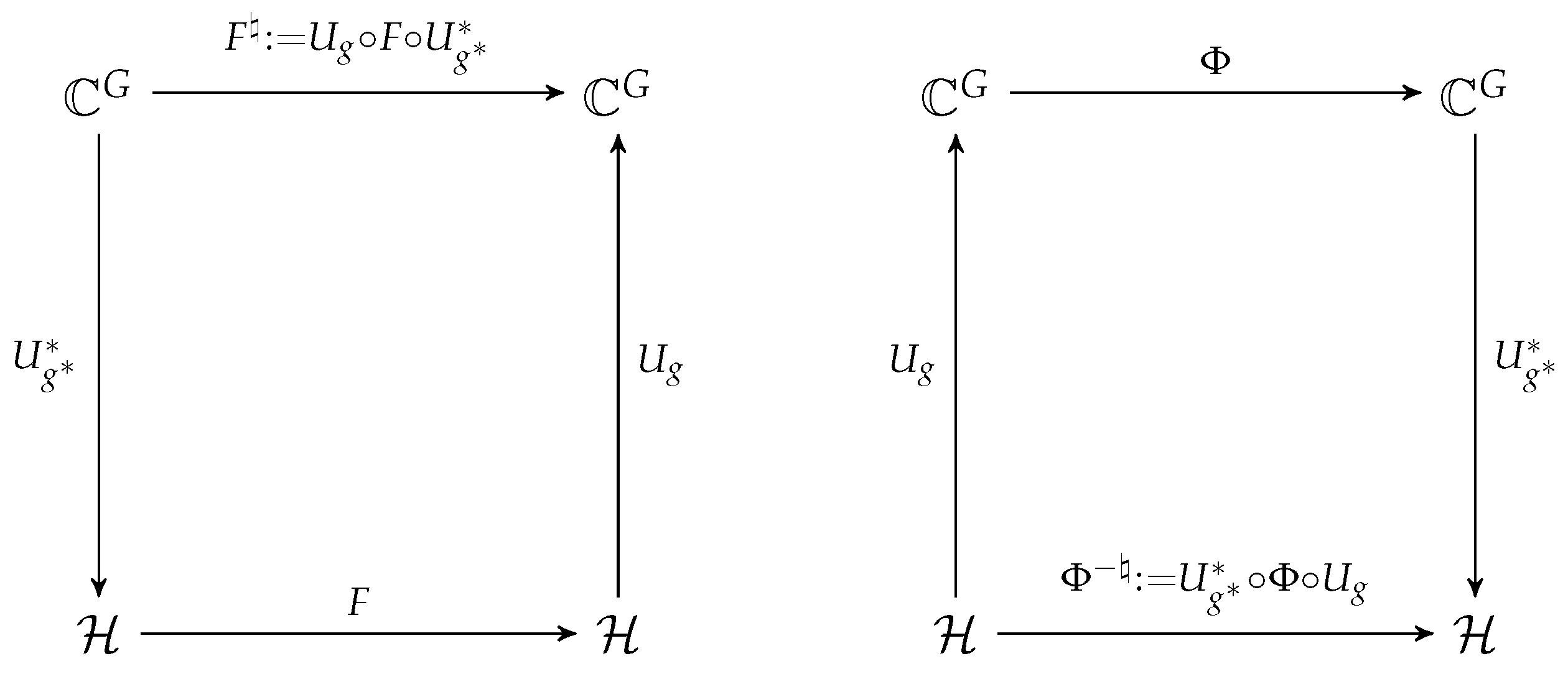
Definition 7.
Let G be a finite group and let ρ be a unitary representation of G on a finite-dimensional Hilbert space H . Assume that span { ρ ( λ ) g : λ G } = H , and let S g : = U g U g and g : = S g 1 ( g ) . For any map F : H H , the ♮-transform of F is defined by
F : = U g F U g : C G C G .
For any map Φ : C G C G , the inverse ♮-transform of Φ is defined by
Φ : = U g Φ U g : H H .
As shown in Figure 1, the ♮-transform converts a map H H into a map C G C G , and the inverse ♮-transform converts a map C G C G into a map H H .
Proposition 4.
Let G be a finite group, and let ρ be a unitary representation of G on a finite-dimensional Hilbert space H . Assume that span { ρ ( λ ) g : λ G } = H , and let S g : = U g U g and g : = S g 1 ( g ) . Then, the following hold.
(i) 
( F ) = F for any map F : H H .
(ii) 
A map F : H H is continuous if and only if F is continuous.
(iii) 
A map F : H H is ( ρ , G ) -equivariant if and only if F is left G-translation equivariant.
Proof. 
(i) It follows from (11) that ( F ) = U g ( U g F U g ) U g = F for any F : H H .
  • (ii) Since the maps U g : H C G and U g : C G H are bounded linear operators, the continuity of F implies the continuity of F = U g F U g . Similarly, the continuity of F implies the continuity of F = ( F ) = U g F U g .
  • (iii) It follows from (10) that the G-equivariance of F implies the left G-translation equivariance of F = U g F U g . Similarly, the left G-translation equivariance of F implies the G-equivariance of F = ( F ) = U g F U g . □
We now provide a brief review of neural networks and the universal approximation theorem.
Let K be either R or C . An activation function is a function σ : K K that acts componentwise on vectors; that is, σ ( x 1 , , x n ) = σ ( x 1 ) , , σ ( x n ) for any ( x 1 , , x n ) K n .
A fully connected feedforward neural network with P hidden layers is given by
Ψ : K d K n , Ψ ( x ) = R ( P ) σ R ( P 1 ) σ R ( 0 ) ,
where R ( p ) : K N p K N p + 1 , x A ( p ) x + b ( p ) is affine-linear with N 0 = d and N P + 1 = n . Such a function Ψ is often called a neural network, but we will call it a σ-neural network to specify the activation function employed.
A shallow neural network is a neural network with a single ( P = 1 ) hidden layer. In particular, a shallow neural network with output dimension n = 1 is given by
Ψ : K d K , Ψ ( x ) = j = 1 J c j σ ( w j T x + b j ) with some J N , c j , b j K , w j K d .
Definition 8.
A function σ : K K is called shallow universal if the set of K -valued shallow σ-networks is dense in the set of all continuous functions f : K d K , with respect to locally uniform convergence.
The following theorem, known as the universal approximation theorem, is a fundamental result in the theory of neural networks.
Theorem 4
(The universal approximation theorem; see [27,28,29,30,31] for K = R , and [32] for K = C ). Let d N .
  • A function σ : R R is shallow universal if and only if σ is not a polynomial.
  • A function σ : C C is shallow universal if and only if σ is not a polyharmonic. Here, a function τ : C C is called polyharmonic if there exists m N such that τ C 2 m in the sense of real variables and Δ m σ 0 , where Δ = 2 x 2 + 2 y 2 is the usual Laplace operator on C R 2 .
In 1996, Mhaskar [33] obtained a quantitative result for approximation of C n functions using shallow networks with smooth activation functions. More recently, Yarotsky [34] derived a quantitative approximation result for deep ReLU networks, where ReLU networks are given by (12) with K = R and the ReLU activation function σ : R R , σ ( x ) = max { x , 0 } , and “deep” refers to having a large P N in (12). For the case of complex-valued deep neural networks, we refer to [35].

3.3. Cyclic Subgroups Λ of Z N × Z N

We now consider the case of cyclic subgroups of Z N × Z N , where group representations can be defined directly without embedding into the Weyl–Heisenberg group. The cyclic subgroups of order N in Z N × Z N are given by
Λ s = { ( 0 , 0 ) , ( 1 , s ) , , ( N 1 , ( N 1 ) s ) } = ( 1 , s ) , s = 0 , , N 1 , Λ = { ( 0 , 0 ) , ( 0 , 1 ) , , ( 0 , N 1 ) } = ( 0 , 1 ) .
If N is prime, these are the only nontrivial proper subgroups of Z N × Z N , but if N is composite, there exist noncyclic subgroups of order N in Z N × Z N ; for instance, { 0 , 2 , 4 } × { 0 , 3 } is a noncyclic subgroup of order 6 in Z 6 × Z 6 . It is easily seen that the adjoint group of Λ s in Z N × Z N is Λ s itself; that is, ( Λ s ) = Λ s (see Section 2.1).
We define the map ρ : Λ s U ( C N ) by
ρ ( k , ) x ( n ) = e k π i / N e 2 π i n / N x ( n k ) , ( k , ) Λ s , x C N .
Setting ω 0 : = e π i / N , we may simply write
ρ ( k , ) = ω 0 k M T k = ω 0 k T k M , ( k , ) Λ s .
For any ( k , ) , ( k , ) Λ s , we have
ρ ( k + k , + ) = ω 0 ( k + ) ( k + ) M + T k + k = ω 0 k k 2 k M + T k + k = ( 8 ) ω 0 k k M T k M T k = ρ ( k , ) ρ ( k , ) ,
where we used the fact that k = k for all ( k , ) , ( k , ) Λ s . This shows that ρ is a group homomorphism and thus a unitary group representation of Λ s on C N . Due the symmetry in (14), ρ is called the symmetric representation of Λ s on C N .
Note that for any F : C N C N and ( k , ) Z N × Z N , we have F π ( k , ) = π ( k , ) F if and only if F ρ ( k , ) = ρ ( k , ) F , where we used the relation ρ ( k , ) = ω 0 k π ( k , ) from (14). This implies that a map F : C N C N is Λ s -equivariant in the sense of Definition 1 if and only if it is ( ρ , Λ s ) -equivariant in the sense of Definition 4. Importantly, employing ( ρ , Λ s ) -equivariance in place of Λ s -equivariance will allow us to apply the tools from group representation theory described in Section 3.2.
We are interested in approximating Λ s -equivariant (or ( ρ , Λ s ) -equivariant) maps F : C N C N by neural networks. For this, we need to choose a complex-valued activation function σ : C C (see Section 3.2) for the neural networks. Since σ acts componentwise on its input, i.e., ( x 1 , , x N ) ( σ ( x N ) , , σ ( x N ) ) , it clearly commutes with all translations, i.e., σ T = T σ ; however, σ does not commute with modulations in general. As shown in (14), the representation ρ includes the multiplicative phase factor ω 0 = e π i / N , so we will assume that σ : C C is e π i / N -phase homogeneous (see Definition 2):
σ ( e π i / N z ) = e π i / N σ ( z ) , z C ,
which ensures that σ commutes with all ρ ( k , ) and all modulations.
We first need the following lemma. Below, we denote by 1 N : = ( 1 , 1 , , 1 ) C N the vector whose entries are all equal to 1.
Lemma 1.
Assume that σ : C C is shallow-universal. If a map F : C N C N satisfies F T = T F , then there exists a shallow convolutional neural network
Ψ : C N C N , Ψ ( x ) = j = 1 J c j σ ( B j x + b j 1 N ) , x C N ,
where B j span { T k : k = 0 , , N 1 } and b j C for j = 1 , , J , which approximates F uniformly on compact sets in C N .
Proof. 
Using the universal approximation theorem (see Theorem 4), the first output component map F 0 : C N C , x ( F x ) ( 0 ) , can be approximated by a shallow network
ψ : C N C , x j = 1 J c j σ ( w j T x + b j )
with some J N , b j , c j C , w j C N . Note that since F T = T F and since T N is the identity map on C N , we have F T n = T n F for all n Z . This condition provides approximations for other component maps F n : C N C , x ( F x ) ( n ) , with n = 1 , , N 1 , in terms of Ψ . In fact, we have
( F x ) ( n ) = ( T n F x ) ( 0 ) = ( F T n x ) ( 0 ) ψ ( T n x ) , x C N , n = 1 , , N 1 .
Consequently, the map F : C N C N , x { ( F x ) ( n ) } n = 0 N 1 , is approximated by the map Ψ : C N C N defined by ( Ψ x ) ( n ) = ψ ( T n x ) for n = 0 , , N 1 . For x , y C N , let x y be the circular convolution of a and b defined by ( x y ) ( n ) = k = 0 N 1 x k y n k , where x and y are understood as N-periodic sequences on the integers. Then, for any x C N and n = 0 , , N 1 , we have
Ψ ( T n x ) = j = 1 J c j σ ( w j x ) ( n ) + b j ,
and therefore, we may write
Ψ : C N C N , Ψ ( x ) = { ψ ( T n x ) } n = 0 N 1 = j = 1 J c j σ ( w j x ) ( n ) + b j n = 0 N 1 .
It is easily seen that every convolutional map C N C N , x w x , is a linear map, and in fact, a linear combination of T k , k = 0 , , N 1 . Hence, the map Ψ : C N C N can be rewritten as
Ψ ( x ) = j = 1 J c j σ ( B j x + b j 1 N ) , x C N ,
where B j span { T k : k = 0 , , N 1 } for j = 1 , , J . The fact that Ψ approximates F uniformly on compact sets in C N follows from the uniform approximation of F 0 by ψ on compact sets in C . Finally, we note that Ψ expressed above is a shallow convolutional neural network described in Section 3.2. This completes the proof. □
Theorem 5.
Assume that σ : C C is shallow universal and satisfies σ ( e π i / N z ) = e π i / N σ ( z ) for all z C . Let Λ = Λ s for some s { 0 , 1 , , N 1 } . Then, any continuous ( ρ , Λ ) -equivariant (or Λ-equivariant) map F : C N C N can be approximated (uniformly on compact sets) by a shallow neural network
x j = 1 J c j σ ( A j x + b j v ) ,
where A j span { ρ ( k , ) : ( k , ) Λ } and b j C for j = 1 , , J , and v C N satisfies ρ ( k , ) v = v for all ( k , ) Λ . Moreover, every map of this form is ( ρ , Λ ) -equivariant (or Λ-equivariant).
Remark 4.
Since ρ ( k , ) = ω 0 k π ( k , ) by (14), we have span { ρ ( k , ) : ( k , ) Λ } = span { π ( k , ) : ( k , ) Λ } for any Λ Z N × Z N . On the other hand, the vectors satisfying ρ ( k , ) b = b can be significantly different from those satisfying π ( k , ) b = b .
Proof. 
Since Λ = Λ s is cyclic, we order its elements as ( 0 , 0 ) , ( 1 , s ) , , ( N 1 , ( N 1 ) s ) , and treat C Λ as C N , since C Λ C N . Then, the operators U g : C N C Λ and U g : C Λ C N , given in Definition 6, can be represented as the N × N matrices
U g = ρ ( 0 , 0 ) g ρ ( N 1 , ( N 1 ) s ) g , U g = ρ ( 0 , 0 ) g , , ρ ( N 1 , ( N 1 ) s ) g ,
respectively, where ( · ) denotes the conjugate transpose. Setting g = ( 1 , 0 , , 0 ) C N , we have
U g = diag ( e k 2 s π i / N ) k = 0 N 1 = 1 0 0 0 e 1 2 s π i / N 0 0 0 e ( N 1 ) 2 s π i / N ,
so that S g = U g U g = Id N and g : = S g 1 g = g . As a result, the set { ρ ( k , ) g } ( k , ) Λ forms an orthonormal basis for C N .
Note that for any continuous ( ρ , Λ ) -equivariant F : C N C N , the map F : = U g F U g : C Λ C Λ is continuous and left Λ -translation equivariant (see Proposition 4). If F is linear, then F is also linear and can be represented as a circulant matrix, equivalently, F = k = 0 N 1 c k T k : C Λ C Λ for some c 0 , , c N 1 C , so that
F = U g ( U g F U g ) U g = U g F U g = k = 0 N 1 c k ( U g T U g ) k .
Therefore, the commutant of ( ρ , Λ ) is given by
C ( ρ , Λ ) : = { F L ( C N ) : F ρ ( k , ) = ρ ( k , ) F for all ( k , ) Λ } = span { U g T k U g : k = 0 , , N 1 } .
On the other hand, since ρ ( k , ) = ω 0 k π ( k , ) by (14), the commutant of ( ρ , Λ ) coincides with that of ( π , Λ ) , i.e.,
C ( ρ , Λ ) = C ( π , Λ ) = ( 4 ) span { π ( k , ) : ( k , ) Λ } = span { ρ ( k , ) : ( k , ) Λ } .
Since the adjoint group of Λ = Λ s is itself, i.e., Λ = Λ (see Section 2.1), we obtain
span { ρ ( k , ) : ( k , ) Λ } = C ( ρ , Λ ) = span { U g T k U g : k = 0 , , N 1 } .
Now, we consider the general case where F : C N C N is possibly nonlinear. If F is nonlinear, then F = U g F U g : C Λ C Λ is a nonlinear left Λ -translation equivariant map. Since Λ = Λ s = { ( 0 , 0 ) , ( 1 , s ) , , ( N 1 , ( N 1 ) s ) } is an additive group and since | Λ | = N and C Λ C N , the map F can be viewed as a map from C N to C N . For simplicity, we will abuse notation and write F : C N C N instead of F : C Λ C Λ ; thus, the first component of F ( x ) C Λ ( C N ) will be simply denoted by ( F x ) ( 0 ) instead of ( F x ) ( 0 , 0 ) . Then, the left Λ -translation equivariance of F can be expressed as F T = T F . By applying Lemma 1 to F : C N C N , we obtain a shallow convolutional neural network
Ψ : C N C N , Ψ ( x ) = j = 1 J c j σ ( B j x + b j 1 N ) , x C N ,
where B j span { T k : k = 0 , , N 1 } , and b j C for j = 1 , , J , which approximates F uniformly on compact sets in C N ; that is,
F ( x ) = ( U g F U g ) ( x ) Ψ ( x ) = j = 1 J c j σ ( B j x + b j 1 N ) x C N .
By the continuity of the operators U g and U g , we obtain
F ( x ) = U g ( U g F U g ) U g ( x ) j = 1 J c j U g σ ( B j U g x + b j 1 N ) , x C N .
Note that since σ ( e π i / N z ) = e π i / N σ ( z ) for all z C , the function σ : C C commutes with U g given by (15), that is, U g σ = σ U g . Therefore, we have
F ( x ) j = 1 J c j σ ( U g B j U g x + b j U g 1 N ) = j = 1 J c j σ ( A j x + b j v ) , x C N ,
where A j : = U g B j U g span { ρ ( k , ) : ( k , ) Λ } by (16), and the vector v : = U g 1 N C N satisfies
ρ ( k , ) v = ρ ( k , ) U g 1 N = ( 4 ) U g L λ 1 N = U g 1 N = v , ( k , ) Λ .
Finally, we note that for any ( k , ) Λ ,
ρ ( k , ) j = 1 J c j σ ( A j x + b j v ) = j = 1 J c j ρ ( k , ) σ ( A j x + b j v ) = j = 1 J c j σ ρ ( k , ) A j x + b j ρ ( k , ) v = j = 1 J c j σ A j ρ ( k , ) x + b j v ,
where we used that ρ ( k , ) is a linear (unitary) operator commuting with σ , and that A j C ( ρ , Λ ) by (16) and ρ ( k , ) v = v by (17). Therefore, every map of the form x j = 1 J c j σ ( A j x + b j v ) is ( ρ , Λ ) -equivariant. □
Remark 5.
The proof relies on observing (16) and choosing g C N such that U g σ = σ U g . To obtain U g σ = σ U g , we have chosen g C N so that U g is a diagonal matrix with exponential entries, and required an appropriate phase-homogeneity on σ so that σ commutes with those exponentials. This technique does not work for Λ because U g cannot be expressed as a diagonal matrix for any g C N in that case.
Example 1.
Let N = 4 and s = 1 , so that Λ = Λ 1 = { ( 0 , 0 ) , ( 1 , 1 ) , ( 2 , 2 ) , ( 3 , 3 ) } Z 4 × Z 4 . In this case, we have ω = e 2 π i / 4 = i , ω 0 = e π i / 4 = 1 2 ( 1 + i ) , and ρ ( k , ) = ω 0 k M T k . Then,
ρ ( 0 , 0 ) = I 4 , ρ ( 1 , 1 ) = ω 0 1 M T = ω 0 1 1 0 0 0 0 i 0 0 0 0 1 0 0 0 0 i 0 0 0 1 1 0 0 0 0 1 0 0 0 0 1 0 = ω 0 1 0 0 0 1 i 0 0 0 0 1 0 0 0 0 i 0 , ρ ( 2 , 2 ) = ω 0 4 M 2 T 2 = 1 0 0 0 0 1 0 0 0 0 1 0 0 0 0 1 0 0 1 0 0 0 0 1 1 0 0 0 0 1 0 0 = 0 0 1 0 0 0 0 1 1 0 0 0 0 1 0 0 , ρ ( 3 , 3 ) = ω 0 9 M 2 T 2 = ω 0 1 1 0 0 0 0 i 0 0 0 0 1 0 0 0 0 i 0 1 0 0 0 0 1 0 0 0 0 1 1 0 0 0 = ω 0 1 0 1 0 0 0 0 i 0 0 0 0 1 i 0 0 0 ,
and ρ ( k , k ) ρ ( k , k ) = ρ ( k + k , k + k ) for all k , k = 0 , 1 , 2 , 3 . With g = ( 1 , 0 , 0 , 0 ) T , we have
U g = ρ ( 0 , 0 ) g ρ ( 1 , 1 ) g ρ ( 2 , 2 ) g ρ ( 3 , 3 ) g = 1 0 0 0 0 ω 0 0 0 0 0 1 0 0 0 0 ω 0 , v : = U g 1 4 = 1 0 0 0 0 ω 0 0 0 0 0 1 0 0 0 0 ω 0 1 1 1 1 = 1 ω 0 1 ω 0 .
It is easy to check that v is invariant under ρ ( 0 , 0 ) , ρ ( 1 , 1 ) , ρ ( 2 , 2 ) , ρ ( 3 , 3 ) ; that is, ρ ( k , k ) v = v for all k = 0 , 1 , 2 , 3 . Theorem 5 shows that any Λ-equivariant map F : C 4 C 4 can be approximated (uniformly on compact sets) by functions of the form
x m = 1 M c m σ ( A m x + b m v ) ,
where A m span { ρ ( k , k ) : k = 0 , 1 , 2 , 3 } and b m C for m = 1 , , M . It is worth noting that while ρ is a unitary group representation of Λ = { ( 0 , 0 ) , ( 1 , 1 ) , ( 2 , 2 ) , ( 3 , 3 ) } on C 4 , the map π | Λ given by π ( k , ) = M T k for ( k , ) Λ is not a group representation of Λ on C 4 , since π ( 1 , 1 ) π ( 1 , 1 ) = ( i ) π ( 2 , 2 ) by (8).

4. Discussion

In this paper, we used finite-dimensional time-frequency analysis to investigate the properties of time-frequency shift equivariant maps that are generally nonlinear.
First, we established a one-to-one correspondence between Λ -equivariant maps and certain phase-homogeneous functions, accompanied by a reconstruction formula expressing Λ -equivariant maps in terms of these functions. This deepens our understanding of the structure of Λ -equivariant maps by connecting them to their corresponding phase-homogeneous functions.
Next, we considered the approximation of Λ -equivariant maps by neural networks. When Λ is a cyclic subgroup of order N in Z N × Z N , we proved that every Λ -equivariant map can be approximated by a shallow neural network with affine linear maps formed as linear combinations of time-frequency shifts by Λ . For the subgroup Λ = ( 1 , 0 ) = { ( 0 , 0 ) , ( 1 , 0 ) , , ( N 1 , 0 ) } , the Λ -equivariance corresponds to translation equivariance, and our result shows that every translation equivariant map can be approximated by a shallow convolutional neural network, which aligns well with the established effectiveness of convolutional neural networks (CNNs) for applications involving translation equivariance. In this context, our result extends the approximation of translation equivariant maps to general Λ -equivariant maps, with potential applications in signal processing.
Finally, we note that the tools used to prove the approximation result (Theorem 2) are applicable in a more general setting than the one described in Section 3.3. In particular, Definitions 6 and 7, and Proposition 4 apply to general unitary representations of arbitrary groups. Therefore, our approach can be adapted to derive similar results for general group-equivariant maps, which we leave as a direction for future research.

Funding

This work was supported by the National Research Foundation of Korea (NRF) grant funded by the Korean government (MSIT) (RS-2023-00275360).

Data Availability Statement

Data are contained within the article.

Acknowledgments

The author would like to thank Andrei Caragea, Johannes Maly, Goetz Pfander, and Felix Voigtlaender for their valuable discussions during the early stages of this paper.

Conflicts of Interest

The author declares no conflicts of interest.

Appendix A. A Proof of the Fact That |Λ°| = L2/|Λ| for Any Subgroup Λ of ℤL × ℤL

For finite abelian groups, it is known (see Lemma 4.2 of [25]) that the adjoint Λ of a subgroup Λ G × G ^ is the symplectic analogue of the dual subgroup Λ , in the sense that Λ = J Λ , where
J = 0 I | G | I | G | 0 .
(In fact, a similar characterization is known for locally compact Abelian groups; see, e.g., Lemma 3.5.9 and Lemma 7.7.3 of [36]. In particular, for separable subgroups Λ = Λ 1 × Λ 2 < G × G ^ , we have Λ = Λ 2 × Λ 1 while Λ = Λ 1 × Λ 2 .) This implies that Λ has the same cardinality as Λ .
Here, the dual (annihilator) H of a subgroup H of G is defined as
H = { m G ^ : m , n = 1 for all n H } ,
where m , n = e 2 π i ( m 1 n 1 / N 1 + + m d n d / N d ) for m = ( m 1 , , m d ) , n = ( n 1 , , n d ) , if G = Z N 1 × × Z N d . It is easily seen that | H | · | H | = | G | , for instance, by taking x = 1 G = ( 1 , 1 , , 1 ) in Theorem 6.3 of [21],
| H | · h H x ( h ) = m H x ^ ( m ) , x C G .
Therefore, we have | Λ | = | Λ | = | Z L × Z L | / | Λ | = L 2 / | Λ | .

References

  1. LeCun, Y.; Bengio, Y.; Hinton, G. Deep learning. Nature 2015, 521, 436–444. [Google Scholar] [CrossRef] [PubMed]
  2. Krizhevsky, A.; Sutskever, I.; Hinton, G.E. ImageNet Classification with Deep Convolutional Neural Networks. In Proceedings of the 26th International Conference on Neural Information Processing Systems, Lake Tahoe, NV, USA, 5–10 December 2013; Pereira, F., Burges, C.J.C., Bottou, L., Weinberger, K.Q., Eds.; Curran Associates, Inc.: Red Hook, NY, USA, 2012; Volume 25. [Google Scholar]
  3. He, K.; Zhang, X.; Ren, S.; Sun, J. Deep residual learning for image recognition. arXiv 2015, arXiv:1512.03385. [Google Scholar]
  4. Hinton, G.; Deng, L.; Yu, D.; Dahl, G.E.; Mohamed, A.; Jaitly, N.; Senior, A.; Vanhoucke, V.; Nguyen, P.; Sainath, T.N.; et al. Deep neural networks for acoustic modeling in speech recognition: The shared views of four research groups. IEEE Signal Process. Mag. 2012, 29, 82–97. [Google Scholar] [CrossRef]
  5. Sutskever, I.; Vinyals, O.; Le, Q.V. Sequence to Sequence Learning with Neural Networks. In Proceedings of the Advances in Neural Information Processing Systems, Montreal, QC, USA, 8–13 December 2014; Ghahramani, Z., Welling, M., Cortes, C., Lawrence, N., Weinberger, K.Q., Eds.; Curran Associates, Inc.: Red Hook, NY, USA, 2014; Volume 27. [Google Scholar]
  6. Vaswani, A.; Shazeer, N.; Parmar, N.; Uszkoreit, J.; Jones, L.; Gomez, A.N.; Kaiser, L.; Polosukhin, I. Attention Is All You Need. In Proceedings of the Advances in Neural Information Processing Systems, Long Beach, CA, USA, 4–9 December 2017; Guyon, I., Luxburg, U.V., Bengio, S., Wallach, H., Fergus, R., Vishwanathan, S., Garnett, R., Eds.; Curran Associates, Inc.: Red Hook, NY, USA, 2017; Volume 30. [Google Scholar]
  7. Silver, D.; Huang, A.; Maddison, C.J.; Guez, A.; Sifre, L.; Van Den Driessche, G.; Schrittwieser, J.; Antonoglou, I.; Panneershelvam, V.; Lanctot, M.; et al. Mastering the game of Go with deep neural networks and tree search. Nature 2016, 529, 484–489. [Google Scholar] [CrossRef] [PubMed]
  8. Hershey, S.; Chaudhuri, S.; Ellis, D.P.W.; Gemmeke, J.F.; Jansen, A.; Moore, R.C.; Plakal, M.; Platt, D.; Saurous, R.A.; Seybold, B.; et al. CNN Architectures for Large-Scale Audio Classification. In Proceedings of the 2017 IEEE International Conference on Acoustics, Speech and Signal Processing (ICASSP), New Orleans, LA, USA, 5–9 March 2017; pp. 131–135. [Google Scholar] [CrossRef]
  9. Oppenheim, A.; Schafer, R. Discrete-Time Signal Processing, 3rd ed.; Pearson: Upper Saddle River, NJ, USA, 2010. [Google Scholar]
  10. Walnut, D. An Introduction to Wavelet Analysis; Birkhäuser: Boston, MA, USA, 2002. [Google Scholar]
  11. Boggess, A.; Narcowich, F.J. A First Course in Wavelets with Fourier Analysis, 2nd ed.; John Wiley & Sons: Hoboken, NJ, USA, 2009. [Google Scholar]
  12. Cohen, T.; Welling, M. Group Equivariant Convolutional Networks. In Proceedings of the 33rd International Conference on Machine Learning, New York, NY, USA, 20–22 June 2016; Volume 48, pp. 2990–2999. [Google Scholar]
  13. Cohen, T.; Geiger, M.; Weiler, M. A general theory of equivariant CNNs on homogeneous spaces. arXiv 2018, arXiv:1811.02017. [Google Scholar]
  14. Yarotsky, D. Universal approximations of invariant maps by neural networks. Constr. Approx. 2022, 55, 407–474. [Google Scholar] [CrossRef]
  15. Cahill, J.; Iverson, J.W.; Mixon, D.G.; Packer, D. Group-invariant max filtering. arXiv 2022, arXiv:2205.14039. [Google Scholar] [CrossRef]
  16. Balan, R.; Tsoukanis, E. G-invariant representations using coorbits: Bi-lipschitz properties. arXiv 2023, arXiv:2308.11784. [Google Scholar]
  17. Balan, R.; Tsoukanis, E. G-invariant representations using coorbits: Injectivity properties. arXiv 2023, arXiv:2310.16365. [Google Scholar]
  18. Huang, N.; Levie, R.; Villar, S. Approximately equivariant graph networks. arXiv 2023, arXiv:2308.10436. [Google Scholar]
  19. Blum-Smith, B.; Villar, S. Machine learning and invariant theory. arXiv 2022, arXiv:2209.14991. [Google Scholar] [CrossRef]
  20. Wang, R.; Walters, R.; Yu, R. Data augmentation vs. equivariant networks: A theory of generalization on dynamics forecasting. arXiv 2022, arXiv:2206.09450. [Google Scholar]
  21. Pfander, G.E. Gabor frames in finite dimensions. In Finite Frames; Casazza, P.G., Kutyniok, G., Eds.; Applied and Numerical Harmonic Analysis; Birkhäuser: Boston, MA, USA, 2013; pp. 193–239. [Google Scholar]
  22. Kaplan, A.; Lee, D.G.; Pfander, G.E.; Pohl, V. Sparse deterministic and stochastic channels: Identification of spreading functions and covariances. In Compressed Sensing in Information Processing; Kutyniok, G., Rauhut, H., Kunsch, R.J., Eds.; Springer International Publishing: New York, NY, USA, 2022; pp. 105–144. [Google Scholar]
  23. Gröchenig, K. Foundations of Time-Frequency Analysis; Applied and Numerical Harmonic Analysis; Birkhäuser: Boston, MA, USA, 2001. [Google Scholar] [CrossRef]
  24. Lawrence, J.; Pfander, G.E.; Walnut, D. Linear independence of Gabor systems in finite dimensional vector spaces. J. Fourier Anal. Appl. 2005, 11, 715–726. [Google Scholar] [CrossRef]
  25. Feichtinger, H.G.; Kozek, W.; Luef, F. Gabor analysis over finite Abelian groups. Appl. Comput. Harmon. Anal. 2009, 26, 230–248. [Google Scholar] [CrossRef]
  26. Christensen, O. An Introduction to Frames and Riesz Bases, 2nd ed.; Birkhäuser: New York, NY, USA, 2016. [Google Scholar]
  27. Cybenko, G. Approximation by superpositions of a sigmoidal function. Math. Control. Signals Syst. 1989, 2, 303–314. [Google Scholar] [CrossRef]
  28. Hornik, K. Approximation capabilities of multilayer feedforward networks. Neural Netw. 1991, 4, 251–257. [Google Scholar] [CrossRef]
  29. Hornik, K.; Stinchcombe, M.; White, H. Multilayer feedforward networks are universal approximators. Neural Netw. 1989, 2, 359–366. [Google Scholar] [CrossRef]
  30. Leshno, M.; Lin, V.; Pinkus, A.; Schocken, S. Multilayer feedforward networks with a nonpolynomial activation function can approximate any function. Neural Netw. 1993, 6, 861–867. [Google Scholar] [CrossRef]
  31. Pinkus, A. Approximation theory of the MLP model in neural networks. Acta Numer. 1999, 8, 143–195. [Google Scholar] [CrossRef]
  32. Voigtlaender, F. The universal approximation theorem for complex-valued neural networks. Appl. Comput. Harmon. Anal. 2023, 64, 33–61. [Google Scholar] [CrossRef]
  33. Mhaskar, H.N. Neural networks for optimal approximation of smooth and analytic functions. Neural Comput. 1996, 8, 164–177. [Google Scholar] [CrossRef]
  34. Yarotsky, D. Error bounds for approximations with deep ReLU networks. Neural Netw. 2017, 94, 103–114. [Google Scholar] [CrossRef] [PubMed]
  35. Caragea, A.; Lee, D.G.; Maly, J.; Pfander, G.E.; Voigtlaender, F. Quantitative approximation results for complex-valued neural networks. SIAM J. Math. Data Sci. 2022, 4, 553–580. [Google Scholar] [CrossRef]
  36. Feichtinger, H.G.; Strohmer, T. (Eds.) Gabor Analysis and Algorithms; Birkhäuser: Boston, MA, USA, 1998. [Google Scholar] [CrossRef]
Figure 1. The ♮-transform and its inverse transform.
Mathematics 12 03704 g001
Disclaimer/Publisher’s Note: The statements, opinions and data contained in all publications are solely those of the individual author(s) and contributor(s) and not of MDPI and/or the editor(s). MDPI and/or the editor(s) disclaim responsibility for any injury to people or property resulting from any ideas, methods, instructions or products referred to in the content.

