
An Efficient Simulated Annealing Algorithm for the Vehicle Routing Problem in Omnichannel Distribution

 ,
,  ,
,  and
and
Abstract
1. Introduction
2. Review of Related Literature
2.1. The Pickup and Delivery Problem in Vehicle Routing
2.2. VRP in Omnichannel Distribution Context

| Year | Authors | VRP Class | Problem Attributes | Solution Approach |
|---|---|---|---|---|
| 2020 | Martins et al. [9] | PD | Handles retail store replenishment and customer deliveries using a shared fleet for both tasks. | Savings-Based Heuristic |
| 2020 | Martins et al. [10] | SPD | Replenishes retail stores and serves direct home deliveries with stochastic travel times. | Simheuristic and Biased-Randomized Heuristic |
| 2020 | Bayliss et al. [11] | MPD | Integrates retailer replenishment and direct home deliveries; combines store replenishment with customer-focused routes. | Discrete-Event Heuristic and Local Search |
| 2020 | Guerrero-Lorente et al. [14] | PD | Manages deliveries and returns across a multi-facility network; supports customer preference with city distribution centers and parcel stations. | Mixed-Integer Programming and Continuous Approximation |
| 2021 | Sawicki et al. [12] | Multi-echelon VRP with Direct Delivery | Serves retail stores and online customers through a two-tier distribution system; focuses on optimizing direct deliveries from central depots and intermediate hubs. | Mixed-integer programming |
| 2021 | Janjevic et al. [13] | Multi-Tier, Multi-Service Level VRP | Replenishes multiple levels of retail inventory; involves replenishing retail stores and satellite hubs, as well as delivering products directly to customers. | Capacitated Location-Routing and Continuum Approximation |
| 2022 | Liu et al. [15] | MPD | Serves retail stores and home customers; integrates replenishment of stores with direct customer deliveries, aiming for cost minimization and customer satisfaction. | Multi-Objective Gray Wolf Optimizer (MOGWO) and Non-dominated Sorting Genetic Algorithm II (NSGA-II) |
| 2022 | Hendalianpour et al. [16] | Multi-product, Multi-level Omnichannel VRP | Replenishes multiple levels of retail inventory; involves replenishing retail stores and satellite hubs, as well as delivering products directly to customers. | Benders Decomposition and Lagrangian Relaxation |
| 2022 | Li et al. [17] | Selective Many-to-Many Pickup and Delivery (SMMPDPH) | Manages selective pickup and delivery among multiple nodes; focuses on minimizing handling costs in omnichannel last-mile delivery. | Mixed-Integer Programming, Iterated Local Search (ILS), and Memetic Algorithm (MA) |
| 2023 | Yang and Li [18] | PD | Performs pickup and delivery between distribution centers, retail stores, and end customers; focuses on efficient transport of heterogeneous goods in omnichannel retail. | Mixed-Integer Programming, Tabu Thresholding and Memetic Algorithms |
| 2025 | Li and Wang [20] | PD | Replenishes retail stores and satellites; manages split deliveries under strict time window constraints for various product types. | Adaptive Large Neighborhood Search (ALNS) |
| 2025 | Qiu et al. [19] | Inventory Replenishment VRP with Capacity-Sharing | Replenishes inventory across retail stores; uses a capacity-sharing strategy to reduce travel and inventory holding costs while meeting online and in-store demands. | Optimization Model and Solution Procedure |
3. Solution Approach
3.1. Solution Encoding
3.2. Initialization
| Algorithm 1: ESA Initialization for the VRPO | |||||||
| Function: Initialize to obtain an initial solution; | |||||||
| Do | |||||||
| A vehicle departs from the depot; | |||||||
| A vehicle travels to the closest unused local store; | |||||||
| Update: (1) vehicle’s current location, (2) vehicle load; | |||||||
| Do | |||||||
| Find the closest unserved customer which satisfies the following conditions: | |||||||
| (1) The current vehicle can provide enough goods for this customer; | |||||||
| (2) If this customer is served and the current vehicle | |||||||
| goes back to the warehouse, it will not violate the max time of the vehicle; | |||||||
| If (one customer is found) { | |||||||
| The current vehicle goes to serve this customer; and | |||||||
| Update current vehicle location and the amount of goods in the vehicle; | |||||||
| Update the partial solution; | |||||||
| } | |||||||
| } Until no unserved customer can be added to the current vehicle route; | |||||||
| The current vehicle goes back to the depot; | |||||||
| Update the partial solution; | |||||||
| } Until all local stores are used | |||||||
3.3. Neighborhood Operators: Swap, Insert, and Invert
3.4. Efficient Simulated Annealing (ESA) Algorithm
| Algorithm 2: ESA for the VRPO | ||||||
| Function: ESA-VRPO to find the best solution, Sbest; | ||||||
| Inputs: T0, Niter, Nnimp, UnitP, beta, and “problem instances”; | ||||||
| begin | ||||||
| Generate initial solution, S ← Initialize; | ||||||
| T ←T0, Sbest←S, Ncount←0, OFVbest← OF(S, UnitP); | ||||||
| While (nimp < Nnimp) do | ||||||
| For iter = 1 to Niter do | ||||||
| Generate prob = uniform (0,1); | ||||||
| If (prob <= ⅓) ←Swap; | ||||||
| If (⅓ < prob <= ⅔) ← Insert; | ||||||
| If (⅔ < prob <= 1) ←Invert; | ||||||
| delta = OF(S′, UnitP)-OF(S, UnitP); | ||||||
| If (delta <= 0) then | ||||||
| S ←S′; | ||||||
| else | ||||||
| Generate lambda = uniform (0,1); | ||||||
| If (lambda <= e(-delta/T)) then | ||||||
| S ←S′; | ||||||
| endif | ||||||
| endif | ||||||
| If (S′ is feasible and OF(S′, UnitP) <= OFVbest) then | ||||||
| Sbest←S′, OFVbest = OF(S′, UnitP), nimp ← 0; | ||||||
| endif | ||||||
| endfor | ||||||
| nimp = nimp +1; T ←T(beta); | ||||||
| endwhile | ||||||
| return Sbest, OFVbest; | ||||||
| end | ||||||
4. Experiment
4.1. Test Instances
4.2. Parameter Setting and Fine-Tuning
4.3. Results and Discussion
4.3.1. Small Instances
4.3.2. Large Instances
- 1.
- Best Know Solutions (BKS): The ESA found fifty-nine new BKS out of sixty large problem instances compared to the 2PH and MAC results. However, for instance b31, MAC’s result remains the BKS (refer to the BKS column).
- 2.
- Performance Comparison Based on BKS: Using the BKS, we calculated the percentage gaps for 2PH and MAC, which are shown in the %Gap (2PH) and %Gap (MAC) columns. Table 7d summarizes the performance improvements of ESA over 2PH and MAC.
- For the ESA-Best results, ESA outperformed 2PH by 78.033%, 80.934%, and 41.853% in low, moderate, and high inventory cases, respectively. For the ESA-Ave results, ESA outperformed 2PH by 75.124%, 77.683%, and 4.941% in the respective cases.
- Against MAC, ESA outperformed with ESA-Best results by 10.185%, 10.478%, and 4.990% for low, moderate, and high inventory cases, respectively. For the ESA-Ave results, ESA outperformed MAC by 7.275%, 7.218%, and 4.077% for each corresponding scenario.
- 3.
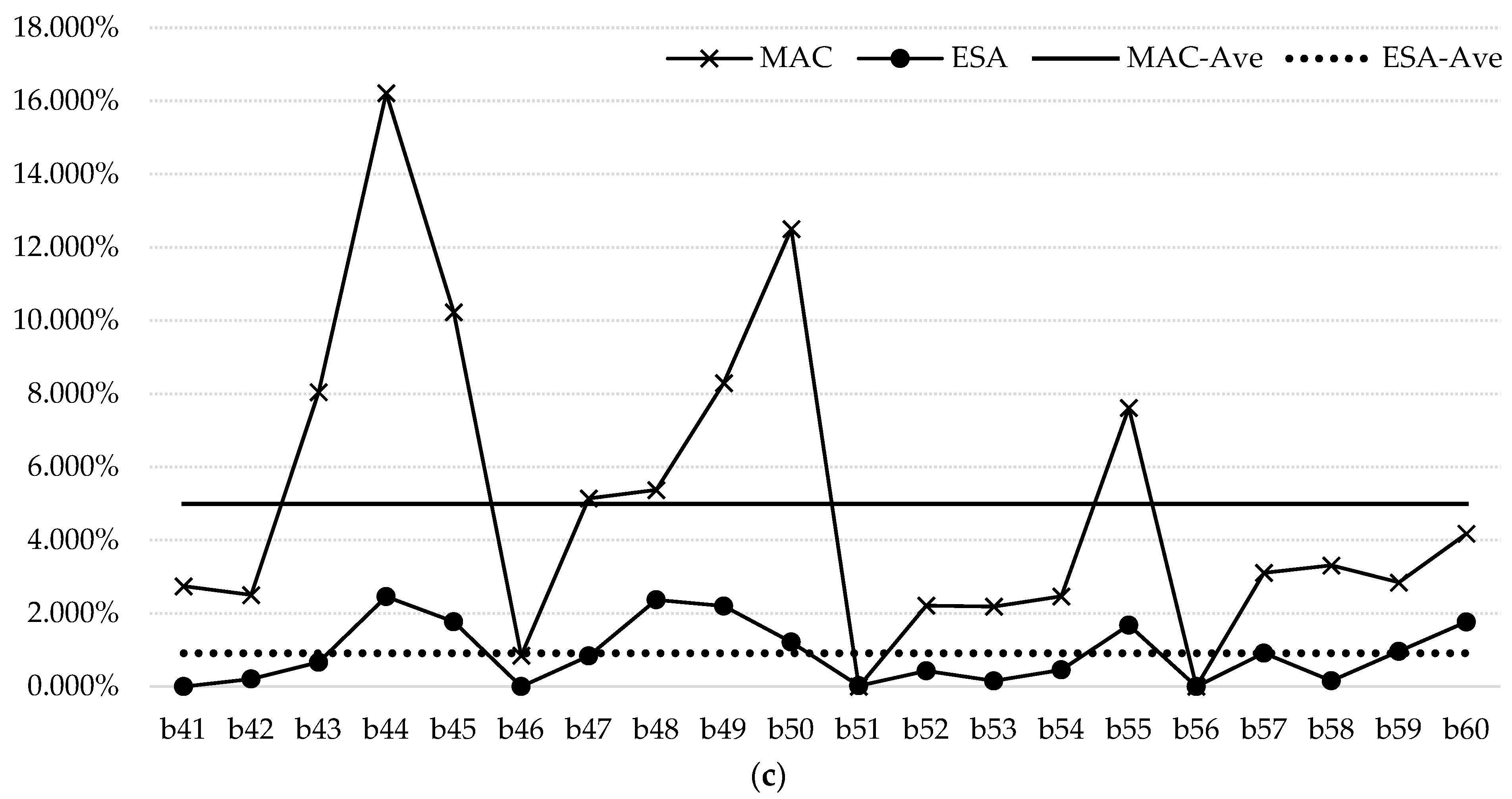
- Stability and Robustness Analysis: To assess the stability and robustness of ESA, we calculated the percentage deviation between the average fitness values (ESA-Ave) and the best solution found (ESA-Best). High-inventory cases exhibited the smallest deviation at 0.913%, indicating strong stability. Deviations for low and moderate cases are 2.909% and 3.275%, respectively, reflecting consistent performance across inventory levels. Figure 2a–c illustrate the percentage gaps of ESA compared to MAC across instances per scenario, showing that ESA consistently maintains greater stability around the average gaps. Additionally, the gaps decrease as the scenarios become more challenging, demonstrating ESA’s robustness.
- 4.
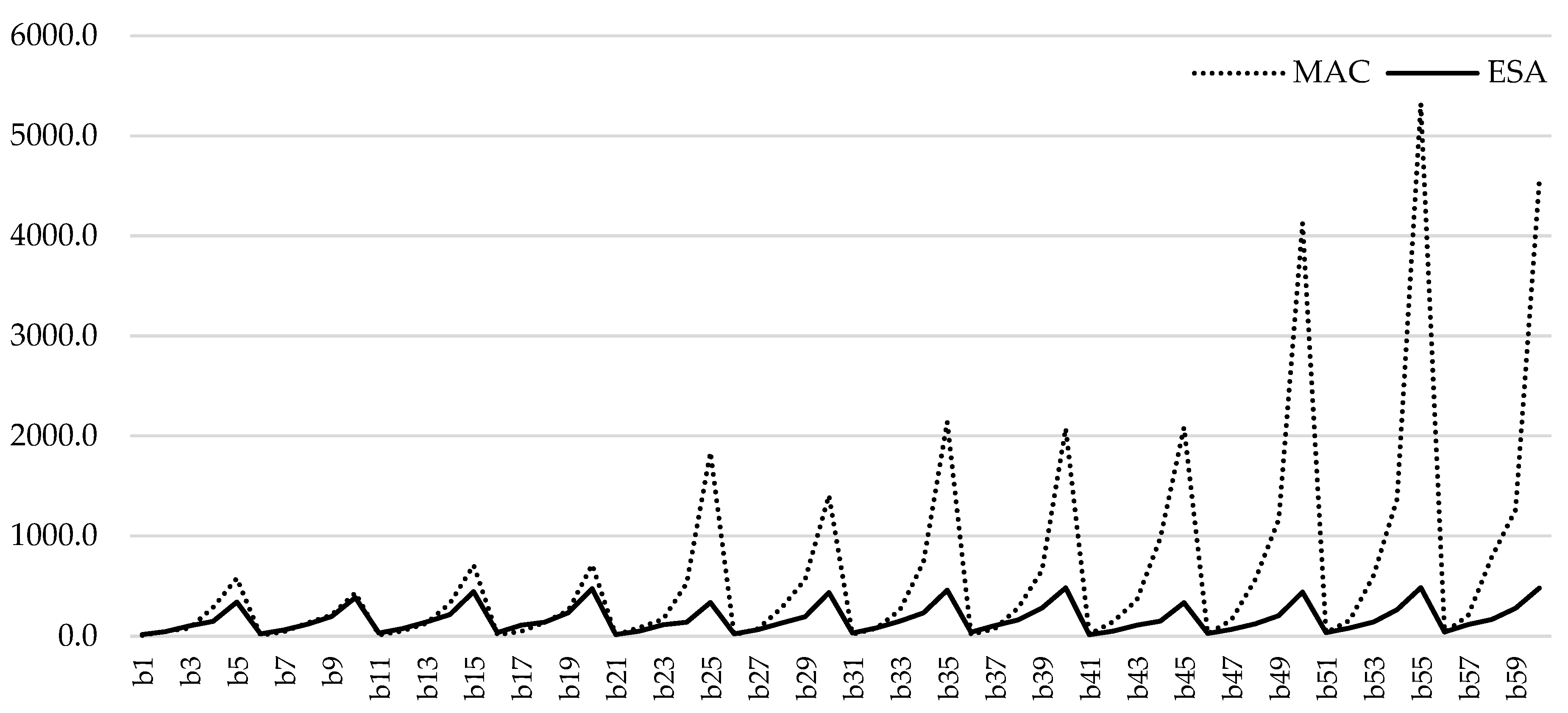
- Average Computational Time: ESA outperformed MAC in 68.33% of the sixty cases. Specifically, ESA demonstrated shorter computation times in 50% of the low inventory cases, 70% of the moderate inventory cases, and 85% of the high inventory cases. As instance difficulty increases ESA’s performance becomes better. Figure 3 compares the computational times of MAC and ESA across three cases. While MAC’s computational time increased significantly with harder instances, ESA maintained a stable trend, demonstrating consistent efficiency and highlighting its scalability and effectiveness.
| (a) | ||||||||||||
|---|---|---|---|---|---|---|---|---|---|---|---|---|
| Ins | BKS | Abdulkader et al. [3] | Efficient Simulated Annealing (ESA) | |||||||||
| 2PH | MAC | Time (sec.) | %Gap (2PH) | %Gap (MAC) | ESA (Best) | ESA (Ave.) | Time (sec.) | %Gap * (Best) | %Gap * (Ave.) | |||
| b1 | 965.658 | 1631.63 | 1002.47 | 7.0 | 68.966% | 3.812% | 965.658 | 972.471 | 14.8 | 0.000% | 0.706% | |
| b2 | 1131.951 | 2057.50 | 1191.97 | 47.0 | 81.766% | 5.302% | 1131.951 | 1175.557 | 44.8 | 0.000% | 3.852% | |
| b3 | 1523.503 | 3006.19 | 1815.42 | 79.0 | 97.321% | 19.161% | 1523.503 | 1600.928 | 102.9 | 0.000% | 5.082% | |
| b4 | 1486.468 | 2830.16 | 1529.04 | 286.0 | 90.395% | 2.864% | 1486.468 | 1582.114 | 145.6 | 0.000% | 6.434% | |
| b5 | 1757.472 | 3478.72 | 1905.19 | 576.0 | 97.939% | 8.405% | 1757.472 | 1800.644 | 339.8 | 0.000% | 2.456% | |
| b6 | 1312.778 | 1774.35 | 1313.69 | 7.0 | 35.160% | 0.069% | 1312.778 | 1345.565 | 20.5 | 0.000% | 2.498% | |
| b7 | 1430.900 | 2461.83 | 1522.29 | 44.0 | 72.048% | 6.387% | 1430.900 | 1446.444 | 62.2 | 0.000% | 1.086% | |
| b8 | 1669.546 | 3545.11 | 2101.77 | 131.0 | 112.340% | 25.889% | 1669.546 | 1726.145 | 119.4 | 0.000% | 3.390% | |
| b9 | 2038.427 | 3528.98 | 2329.53 | 209.0 | 73.123% | 14.281% | 2038.427 | 2118.569 | 196.1 | 0.000% | 3.932% | |
| b10 | 2314.624 | 4916.75 | 3012.18 | 430.0 | 112.421% | 30.137% | 2314.624 | 2413.788 | 384.2 | 0.000% | 4.284% | |
| b11 | 1574.268 | 2432.56 | 1611.34 | 11.0 | 54.520% | 2.355% | 1574.268 | 1592.868 | 29.4 | 0.000% | 1.182% | |
| b12 | 1720.667 | 2695.34 | 1800.87 | 50.0 | 56.645% | 4.661% | 1720.667 | 1773.679 | 73.9 | 0.000% | 3.081% | |
| b13 | 2406.040 | 3936.67 | 2406.04 | 127.0 | 92.430% | 17.611% | 2045.768 | 2078.285 | 140.6 | 0.000% | 1.589% | |
| b14 | 2227.445 | 3826.14 | 2483.81 | 327.0 | 71.773% | 11.509% | 2227.445 | 2292.73 | 214.5 | 0.000% | 2.931% | |
| b15 | 2432.789 | 4496.05 | 2679.15 | 708.0 | 84.811% | 10.127% | 2432.789 | 2498.48 | 443.2 | 0.000% | 2.700% | |
| b16 | 1630.361 | 2254.87 | 1669.56 | 13.0 | 38.305% | 2.404% | 1630.361 | 1648.857 | 33.2 | 0.000% | 1.134% | |
| b17 | 1904.518 | 3020.80 | 1965.56 | 46.0 | 58.612% | 3.205% | 1904.518 | 1928.351 | 109.1 | 0.000% | 1.251% | |
| b18 | 2279.020 | 3963.52 | 2449.76 | 136.0 | 73.913% | 7.492% | 2279.020 | 2354.603 | 138.3 | 0.000% | 3.316% | |
| b19 | 2412.603 | 4933.86 | 2788.48 | 257.0 | 104.504% | 15.580% | 2412.603 | 2501.918 | 233.5 | 0.000% | 3.702% | |
| b20 | 2570.524 | 4721.26 | 2890.29 | 712.0 | 83.669% | 12.440% | 2570.524 | 2662.451 | 474.0 | 0.000% | 3.576% | |
| Ave. | 210.1 | 78.033% | 10.185% | 166.0 | 0.000% | 2.909% | ||||||
| (b) | ||||||||||||
| Ins | BKS | Abdulkader et al. [3] | Efficient Simulated Annealing (ESA) | |||||||||
| 2PH | MAC | Time (sec.) | %Gap (2PH) | %Gap (MAC) | ESA (Best) | ESA (Ave.) | Time (sec.) | %Gap * (Best) | %Gap * (Ave.) | |||
| b21 | 830.576 | 1571.63 | 879.16 | 10.0 | 89.222% | 5.849% | 830.576 | 838.639 | 15.0 | 0.000% | 0.971% | |
| b22 | 985.593 | 1920.59 | 1083.66 | 85.0 | 94.866% | 9.950% | 985.593 | 1007.615 | 49.2 | 0.000% | 2.234% | |
| b23 | 1307.761 | 2699.23 | 1591.52 | 167.0 | 106.401% | 21.698% | 1307.761 | 1356.962 | 111.7 | 0.000% | 3.762% | |
| b24 | 1180.631 | 2305.09 | 1437.68 | 528.0 | 95.242% | 21.772% | 1180.631 | 1267.620 | 138.9 | 0.000% | 7.368% | |
| b25 | 1341.064 | 2700.41 | 1520.51 | 1836.0 | 101.363% | 13.381% | 1341.064 | 1421.077 | 336.2 | 0.000% | 5.966% | |
| b26 | 1177.616 | 1665.15 | 1180.83 | 11.0 | 41.400% | 0.273% | 1177.616 | 1182.247 | 21.2 | 0.000% | 0.393% | |
| b27 | 1326.928 | 2320.66 | 1329.26 | 73.0 | 74.890% | 0.176% | 1326.928 | 1348.179 | 62.9 | 0.000% | 1.602% | |
| b28 | 1504.426 | 3016.45 | 1692.41 | 279.0 | 100.505% | 12.495% | 1504.426 | 1586.755 | 129.2 | 0.000% | 5.472% | |
| b29 | 1685.024 | 3302.39 | 2016.40 | 567.0 | 95.985% | 19.666% | 1685.024 | 1779.461 | 193.3 | 0.000% | 5.604% | |
| b30 | 1812.834 | 3918.97 | 2399.60 | 1407.0 | 116.179% | 32.367% | 1812.834 | 1970.385 | 435.6 | 0.000% | 8.691% | |
| b31 | 1495.790 | 1993.49 | 1495.79 | 16.0 | 33.273% | 0.000% | 1500.196 | 1514.549 | 29.9 | 0.295% | 1.254% | |
| b32 | 1583.288 | 2713.01 | 1656.86 | 76.0 | 71.353% | 4.647% | 1583.288 | 1604.756 | 80.6 | 0.000% | 1.356% | |
| b33 | 1715.007 | 3393.34 | 1799.64 | 262.0 | 97.862% | 4.935% | 1715.007 | 1772.595 | 147.7 | 0.000% | 3.358% | |
| b34 | 1821.977 | 3127.49 | 2018.50 | 740.0 | 71.654% | 10.786% | 1821.977 | 1883.839 | 230.5 | 0.000% | 3.395% | |
| b35 | 2008.901 | 3742.21 | 2290.95 | 2141.0 | 86.281% | 14.040% | 2008.901 | 2092.139 | 458.0 | 0.000% | 4.143% | |
| b36 | 1496.488 | 2032.06 | 1550.01 | 15.0 | 35.789% | 3.577% | 1496.488 | 1518.099 | 37.3 | 0.000% | 1.444% | |
| b37 | 1833.898 | 3130.52 | 1939.50 | 73.0 | 70.703% | 5.758% | 1833.898 | 1880.449 | 104.1 | 0.000% | 2.538% | |
| b38 | 1944.259 | 3433.23 | 2088.58 | 283.0 | 76.583% | 7.423% | 1944.259 | 1964.290 | 162.2 | 0.000% | 1.030% | |
| b39 | 1996.767 | 3824.46 | 2244.14 | 656.0 | 91.533% | 12.389% | 1996.767 | 2023.750 | 280.6 | 0.000% | 1.351% | |
| b40 | 2051.460 | 3447.89 | 2229.43 | 2077.0 | 68.070% | 8.675% | 2051.460 | 2124.600 | 480.9 | 0.000% | 3.565% | |
| Ave. | 565.1 | 80.958% | 10.493% | 175.3 | 0.015% | 3.275% | ||||||
| (c) | ||||||||||||
| Ins | BKS | Abdulkader et al. [3] | Efficient Simulated Annealing (ESA) | |||||||||
| 2PH | MAC | Time (sec.) | %Gap (2PH) | %Gap (MAC) | ESA (Best) | ESA (Ave.) | Time (sec.) | %Gap (Best) | %Gap (Ave.) | |||
| b41 | 692.317 | 897.55 | 711.29 | 16.0 | 29.644% | 2.741% | 692.317 | 692.317 | 14.7 | 0.000% | 0.000% | |
| b42 | 853.859 | 1287.81 | 875.24 | 143.0 | 50.822% | 2.504% | 853.859 | 855.624 | 49.2 | 0.000% | 0.207% | |
| b43 | 1047.763 | 1531.06 | 1132.05 | 358.0 | 46.127% | 8.044% | 1047.763 | 1054.713 | 108.8 | 0.000% | 0.663% | |
| b44 | 1053.330 | 1636.54 | 1224.11 | 978.0 | 55.368% | 16.213% | 1053.330 | 1079.247 | 148.9 | 0.000% | 2.460% | |
| b45 | 1155.630 | 1551.75 | 1273.86 | 2085.0 | 34.277% | 10.231% | 1155.630 | 1176.100 | 332.5 | 0.000% | 1.771% | |
| b46 | 988.557 | 1264.32 | 996.93 | 22.0 | 27.896% | 0.847% | 988.557 | 988.557 | 26.1 | 0.000% | 0.000% | |
| b47 | 1027.516 | 1488.07 | 1080.34 | 159.0 | 44.822% | 5.141% | 1027.516 | 1036.107 | 66.3 | 0.000% | 0.836% | |
| b48 | 1188.503 | 1815.22 | 1252.35 | 559.0 | 52.732% | 5.372% | 1188.503 | 1216.658 | 121.3 | 0.000% | 2.369% | |
| b49 | 1471.915 | 2242.40 | 1594.02 | 1167.0 | 52.346% | 8.296% | 1471.915 | 1504.279 | 203.3 | 0.000% | 2.199% | |
| b50 | 1503.470 | 2459.52 | 1691.42 | 4126.0 | 63.590% | 12.501% | 1503.470 | 1521.713 | 439.8 | 0.000% | 1.213% | |
| b51 | 1302.884 | 1660.91 | 1302.89 | 33.0 | 27.479% | 0.000% | 1302.884 | 1303.162 | 33.7 | 0.000% | 0.021% | |
| b52 | 1272.812 | 1740.66 | 1300.98 | 156.0 | 36.757% | 2.213% | 1272.812 | 1278.270 | 80.2 | 0.000% | 0.429% | |
| b53 | 1391.373 | 2096.76 | 1421.77 | 605.0 | 50.697% | 2.185% | 1391.373 | 1393.505 | 139 | 0.000% | 0.153% | |
| b54 | 1601.141 | 2226.39 | 1640.60 | 1370.0 | 39.050% | 2.464% | 1601.141 | 1608.418 | 263.5 | 0.000% | 0.454% | |
| b55 | 1638.572 | 2518.16 | 1763.31 | 5321.0 | 53.680% | 7.613% | 1638.572 | 1666.076 | 484.8 | 0.000% | 1.679% | |
| b56 | 1311.628 | 1550.71 | 1311.63 | 36.0 | 18.228% | 0.000% | 1311.628 | 1311.628 | 39.9 | 0.000% | 0.000% | |
| b57 | 1423.865 | 1835.39 | 1468.12 | 203.0 | 28.902% | 3.108% | 1423.865 | 1436.874 | 113.7 | 0.000% | 0.914% | |
| b58 | 1601.873 | 2276.94 | 1654.92 | 791.0 | 42.142% | 3.312% | 1601.873 | 1604.410 | 166.5 | 0.000% | 0.158% | |
| b59 | 1532.106 | 2061.86 | 1575.67 | 1262.0 | 34.577% | 2.843% | 1532.106 | 1546.861 | 277.8 | 0.000% | 0.963% | |
| b60 | 1587.046 | 2347.76 | 1653.30 | 4549.0 | 47.933% | 4.175% | 1587.046 | 1615.076 | 478.5 | 0.000% | 1.766% | |
| Ave. | 1196.9 | 41.853% | 4.990% | 179.4 | 0.000% | 0.913% | ||||||
| (d) | ||||||||||||
| Mean %Gaps w.r.t. BKS per Scenario | ESA Outperforms 2PH by: | ESA Outperforms MAC by: | ||||||||||
| Case | ESA (Best) | ESA (Ave) | 2PH | MAC | ESA (Best) | ESA (Ave) | ESA (Best) | ESA (Ave) | ||||
| Low | 0.000% | 2.909% | 78.033% | 10.185% | −78.033% | −75.124% | −10.185% | −7.275% | ||||
| Moderate | 0.015% | 3.275% | 80.958% | 10.493% | −80.943% | −77.683% | −10.478% | −7.218% | ||||
| High | 0.000% | 0.913% | 41.853% | 4.990% | −41.853% | −40.941% | −4.990% | −4.077% | ||||

5. Summary and Conclusions
Author Contributions
Funding
Data Availability Statement
Conflicts of Interest
References
- Lokin, F.C.J. Procedures for Travelling Salesman Problems with Additional Constraints. Eur. J. Oper. Res. 1979, 3, 135–141. [Google Scholar] [CrossRef]
- Berbeglia, G.; Cordeau, J.-F.; Gribkovskaia, I.; Laporte, G. Static Pickup and Delivery Problems: A Classification Scheme and Survey. TOP 2007, 15, 1–31. [Google Scholar] [CrossRef]
- Abdulkader, M.M.S.; Gajpal, Y.; ElMekkawy, T.Y. Vehicle Routing Problem in Omni-Channel Retailing Distribution Systems. Int. J. Prod. Econ. 2018, 196, 43–55. [Google Scholar] [CrossRef]
- Braekers, K.; Caris, A.; Janssens, G.K. Exact and Meta-Heuristic Approach for a General Heterogeneous Dial-a-Ride Problem with Multiple Depots. Transp. Res. Part B Methodol. 2014, 67, 166–186. [Google Scholar] [CrossRef]
- Parragh, S.N.; Doerner, K.F.; Hartl, R.F. A Survey on Pickup and Delivery Problems. Part I: Transportation Between Customers and Depot. J. Für Betriebswirtschaft 2008, 58, 21–51. [Google Scholar] [CrossRef]
- Battarra, M.; Cordeau, J.-F.; Iori, M. Chapter 6: Pickup-and-Delivery Problems for Goods Transportation. In Vehicle Routing: Problems, Methods, and Applications; MOS-SIAM Series on Optimization; Society for Industrial and Applied Mathematics: Philadelphia, PA, USA, 2014; pp. 161–191. [Google Scholar]
- Parragh, S.N.; Doerner, K.F.; Hartl, R.F. A Survey on Pickup and Delivery Problems: Part II: Transportation Between Pickup and Delivery Locations. J. Für Betriebswirtschaft 2008, 58, 81–117. [Google Scholar] [CrossRef]
- Beck, N.; Rygl, D. Categorization of Multiple Channel Retailing in Multi-, Cross-, and Omni-Channel Retailing for Retailers and Retailing. J. Retail. Consum. Serv. 2015, 27, 170–178. [Google Scholar] [CrossRef]
- Martins, L.D.C.; Bayliss, C.; Juan, A.A.; Panadero, J.; Marmol, M. A Savings-Based Heuristic for Solving the Omnichannel Vehicle Routing Problem with Pick-up and Delivery. Transp. Res. Procedia 2020, 47, 83–90. [Google Scholar] [CrossRef]
- Martins, L.D.C.; Bayliss, C.; Copado-Méndez, P.J.; Panadero, J.; Juan, A.A. A Simheuristic Algorithm for Solving the Stochastic Omnichannel Vehicle Routing Problem with Pick-up and Delivery. Algorithms 2020, 13, 237. [Google Scholar] [CrossRef]
- Bayliss, C.; Martins, L.d.C.; Juan, A.A. A Two-Phase Local Search with a Discrete-Event Heuristic for the Omnichannel Vehicle Routing Problem. Comput. Ind. Eng. 2020, 148, 106695. [Google Scholar] [CrossRef]
- Sawicki, P.; Sawicka, H. Optimisation of the Two-Tier Distribution System in Omni-Channel Environment. Energies 2021, 14, 7700. [Google Scholar] [CrossRef]
- Janjevic, M.; Merchán, D.; Winkenbach, M. Designing Multi-Tier, Multi-Service-Level, and Multi-Modal Last-Mile Distribution Networks for Omni-Channel Operations. Eur. J. Oper. Res. 2021, 294, 1059–1077. [Google Scholar] [CrossRef]
- Guerrero-Lorente, J.; Gabor, A.F.; Ponce-Cueto, E. Omnichannel Logistics Network Design with Integrated Customer Preference for Deliveries and Returns. Comput. Ind. Eng. 2020, 144, 106433. [Google Scholar] [CrossRef]
- Liu, P.; Hendalianpour, A.; Feylizadeh, M.; Pedrycz, W. Mathematical Modeling of Vehicle Routing Problem in Omni-Channel Retailing. Appl. Soft Comput. 2022, 131, 109791. [Google Scholar] [CrossRef]
- Hendalianpour, A.; Fakhrabadi, M.; Sangari, M.S.; Razmi, J. A Combined Benders Decomposition and Lagrangian Relaxation Algorithm for Optimizing a Multi-Product, Multi-Level Omni-Channel Distribution System. Sci. Iran. 2022, 29, 355–371. [Google Scholar] [CrossRef]
- Li, Y. A Selective Many-to-Many Pickup and Delivery Problem with Handling Cost in the Omni-Channel Last-Mile Delivery. IEEE Access 2022, 10, 111284–111296. [Google Scholar] [CrossRef]
- Yang, J.; Li, Y. A Multicommodity Pickup and Delivery Problem with Time Windows and Handling Time in the Omni-Channel Last-Mile Delivery. Int. Trans. Oper. Res. 2023. [Google Scholar] [CrossRef]
- Qiu, R.; Yuan, M.; Sun, M.; Fan, Z.P.; Xu, H. Optimizing Omnichannel Retailer Inventory Replenishment Using Vehicle Capacity-Sharing with Demand Uncertainties and Service Level Requirements. Eur. J. Oper. Res. 2025, 320, 417–432. [Google Scholar] [CrossRef]
- Li, N.; Wang, Z. Vehicle Routing Problem for Omnichannel Retailing Including Multiple Types of Time Windows and Products. Comput. Oper. Res. 2025, 173, 106828. [Google Scholar] [CrossRef]
- Wang, C.; Mu, D.; Zhao, F.; Sutherland, J.W. A Parallel Simulated Annealing Method for the Vehicle Routing Problem with Simultaneous Pickup-Delivery and Time Windows. Comput. Ind. Eng. 2015, 83, 111–122. [Google Scholar] [CrossRef]
- Avci, M.; Topaloglu, S. An Adaptive Local Search Algorithm for Vehicle Routing Problem with Simultaneous and Mixed Pickups and Deliveries. Comput. Ind. Eng. 2015, 83, 15–29. [Google Scholar] [CrossRef]
- Danloup, N.; Allaoui, H.; Goncalves, G. A Comparison of Two Meta-Heuristics for the Pickup and Delivery Problem with Transshipment. Comput. Oper. Res. 2018, 100, 155–171. [Google Scholar] [CrossRef]
- Koç, Ç.; Laporte, G.; Tükenmez, İ. A Review of Vehicle Routing with Simultaneous Pickup and Delivery. Comput. Oper. Res. 2020, 122, 104987. [Google Scholar] [CrossRef]
- Kirkpatrick, S.; Gelatt, C.D.; Vecchi, M.P. Optimization by Simulated Annealing. Science 1983, 220, 671–680. [Google Scholar] [CrossRef]
- İlhan, İ. An Improved Simulated Annealing Algorithm with Crossover Operator for Capacitated Vehicle Routing Problem. Swarm Evol. Comput. 2021, 64, 100911. [Google Scholar] [CrossRef]
- Lin, S.W.; Cheng, C.Y.; Pourhejazy, P.; Ying, K.C. Multi-Temperature Simulated Annealing for Optimizing Mixed-Blocking Permutation Flowshop Scheduling Problems. Expert Syst. Appl. 2021, 165, 113837. [Google Scholar] [CrossRef]
- Yu, V.F.; Anh, P.T.; Gunawan, A.; Han, H. A Simulated Annealing with Variable Neighborhood Descent Approach for the Heterogeneous Fleet Vehicle Routing Problem with Multiple Forward/Reverse Cross-Docks. Expert Syst. Appl. 2024, 237, 121631. [Google Scholar] [CrossRef]
- Leite, N.; Melício, F.; Rosa, A.C. A Fast Simulated Annealing Algorithm for the Examination Timetabling Problem. Expert Syst. Appl. 2019, 122, 137–151. [Google Scholar] [CrossRef]
- Rodríguez-Esparza, E.; Masegosa, A.D.; Oliva, D.; Onieva, E. A New Hyper-Heuristic Based on Adaptive Simulated Annealing and Reinforcement Learning for the Capacitated Electric Vehicle Routing Problem. Expert Syst. Appl. 2024, 252, 124197. [Google Scholar] [CrossRef]
- Yu, V.F.; Indrakarna, P.A.Y.; Ngurah, A.A.; Redi, P.; Lin, S.-W. Simulated Annealing with Mutation Strategy for the Share-a-Ride Problem with Flexible Compartments. Mathematics 2021, 9, 2320. [Google Scholar] [CrossRef]
- Lin, S.W.; Yu, V.F. Solving the Team Orienteering Problem with Time Windows and Mandatory Visits by Multi-Start Simulated Annealing. Comput. Ind. Eng. 2017, 114, 195–205. [Google Scholar] [CrossRef]
- Ying, K.C.; Lin, S.W. Minimizing Total Completion Time in the No-Wait Jobshop Scheduling Problem Using a Backtracking Metaheuristic. Comput. Ind. Eng. 2022, 169, 108238. [Google Scholar] [CrossRef]
- Lin, S.W.; Cheng, C.Y.; Pourhejazy, P.; Ying, K.C.; Lee, C.H. New Benchmark Algorithm for Hybrid Flowshop Scheduling with Identical Machines. Expert Syst. Appl. 2021, 183, 115422. [Google Scholar] [CrossRef]
- Yu, V.F.; Susanto, H.; Yeh, Y.-H.; Lin, S.-W.; Huang, Y.-T. The Vehicle Routing Problem with Simultaneous Pickup and Delivery and Parcel Lockers. Mathematics 2022, 10, 920. [Google Scholar] [CrossRef]
- Stamadianos, T.; Kyriakakis, N.A.; Marinaki, M.; Marinakis, Y. A Hybrid Simulated Annealing and Variable Neighborhood Search Algorithm for the Close-Open Electric Vehicle Routing Problem. Ann. Math. Artif. Intell. 2023. [Google Scholar] [CrossRef]
- Xiao, S.; Peng, P.; Zheng, P.; Wu, Z. A Hybrid Adaptive Simulated Annealing and Tempering Algorithm for Solving the Half-Open Multi-Depot Vehicle Routing Problem. Mathematics 2024, 12, 947. [Google Scholar] [CrossRef]
| Case | Stock Availability | Description |
|---|---|---|
| (1) Low | Total stock in the network exceeds consumer demand by 10–20%. | |
| (2) Moderate | Inventory exceeds demand by 50–100%. | |
| (3) High | Each store’s stock can fully meet all demands across the network. |
| Parameter | Definition | Levels |
|---|---|---|
| T0 | Initial temperature | 10, 20, 30, 40 |
| Niter | Number of iterations per T level | 2000 L, 2500 L, 3000 L, 3500 L |
| beta | Cooling coefficient | 0.90, 0.93, 0.96, 0.99 |
| Nnimp | Maximum iterations over non-improving solutions | 20, 30, 40, 50 |
| UnitP | Unit penalty per constraint violation | 1500, 2000, 2500, 3000 |
| Combinations | T0 | Niter | beta | Nnimp | UnitP | %Gap * (Ave.) | Time (Ave.) |
|---|---|---|---|---|---|---|---|
| 1 | 10 | 2000 L | 0.90 | 20 | 1500 | 8.561 | 28.87 |
| 2 | 10 | 2500 L | 0.93 | 30 | 2000 | 7.524 | 49.28 |
| 3 | 10 | 3000 L | 0.96 | 40 | 2500 | 6.161 | 91.06 |
| 4 | 10 | 3500 L | 0.99 | 50 | 3000 | 4.164 | 279.94 |
| 5 | 20 | 2000 L | 0.93 | 40 | 3000 | 7.191 | 49.56 |
| 6 | 20 | 2500 L | 0.90 | 50 | 2500 | 7.548 | 57.93 |
| 7 | 20 | 3000 L | 0.99 | 20 | 2000 | 6.810 | 202.49 |
| 8 | 20 | 3500 L | 0.96 | 30 | 1500 | 5.060 | 109.09 |
| 9 | 30 | 2000 L | 0.96 | 50 | 2000 | 5.847 | 79.33 |
| 10 | 30 | 2500 L | 0.99 | 40 | 1500 | 4.795 | 252.13 |
| 11 | 30 | 3000 L | 0.90 | 30 | 3000 | 6.682 | 54.22 |
| 12 | 30 | 3500 L | 0.93 | 20 | 2500 | 5.634 | 68.91 |
| 13 | 40 | 2000 L | 0.99 | 30 | 2500 | 8.863 | 176.05 |
| 14 | 40 | 2500 L | 0.96 | 20 | 3000 | 5.803 | 78.35 |
| 15 | 40 | 3000 L | 0.93 | 50 | 1500 | 6.116 | 85.33 |
| 16 | 40 | 3500 L | 0.90 | 40 | 2000 | 6.155 | 72.60 |
| Levels | %Gap (Ave.) | Time (Ave.) | |||||||||
|---|---|---|---|---|---|---|---|---|---|---|---|
| T0 | Niter | beta | Nnimp | UnitP | T0 | Niter | beta | Nnimp | UnitP | ||
| 1 | 6.6025 | 7.6154 | 7.2365 | 6.7021 | 6.1330 | 107.26 | 81.71 | 52.46 | 92.06 | 114.50 | |
| 2 | 6.6522 | 6.4177 | 6.6164 | 7.0323 | 6.5843 | 100.09 | 105.42 | 62.18 | 95.40 | 97.22 | |
| 3 | 5.7398 | 6.4424 | 5.7177 | 6.0756 | 7.0516 | 109.94 | 104.98 | 86.35 | 111.95 | 96.84 | |
| 4 | 6.7344 | 5.2535 | 6.1583 | 5.9189 | 5.9601 | 103.08 | 128.27 | 219.39 | 120.97 | 111.82 | |
| Range | 0.9946 | 2.3619 | 1.5188 | 1.1134 | 1.0915 | 9.85 | 46.56 | 166.93 | 28.90 | 17.66 | |
| Rank | 5 | 1 | 2 | 3 | 4 | 5 | 2 | 1 | 3 | 4 | |
| MINLP by Gurobi | Abdulkader et al. [3] | ESA | ||||||||||
|---|---|---|---|---|---|---|---|---|---|---|---|---|
| Ins | Optimal | Time (sec.) | 2PH | %Gap | MAC | %Gap | ESA (Best) | ESA (Ave.) | Time (Ave.) | %Gap * (Best) | %Gap * (Ave.) | |
| a1 | 386.906 | 0.11 | 479.19 | 23.85 | 386.91 | 0.00 | 386.906 | 386.906 | 1.00 | 0.00 | 0.00 | |
| a2 | 416.346 | 1.31 | 589.63 | 41.62 | 416.35 | 0.00 | 416.346 | 416.346 | 1.50 | 0.00 | 0.00 | |
| a3 | 424.309 | 5.27 | 512.32 | 20.74 | 424.31 | 0.00 | 424.309 | 424.309 | 2.40 | 0.00 | 0.00 | |
| a4 | 455.288 | 28.70 | 767.06 | 68.48 | 455.29 | 0.00 | 455.288 | 455.288 | 3.80 | 0.00 | 0.00 | |
| a5 | 601.363 | 179.55 | 936.20 | 55.68 | 601.36 | 0.00 | 601.363 | 702.640 | 4.90 | 0.00 | 16.84 | |
| a6 | 419.327 | 2.16 | 512.12 | 22.13 | 419.32 | 0.00 | 419.327 | 419.327 | 1.20 | 0.00 | 0.00 | |
| a7 | 455.912 | 14.66 | 688.39 | 50.99 | 455.91 | 0.00 | 455.912 | 455.912 | 1.80 | 0.00 | 0.00 | |
| a8 | 448.831 | 153.45 | 711.89 | 58.61 | 449.35 | 0.12 | 448.831 | 448.831 | 2.80 | 0.00 | 0.00 | |
| a9 | 457.319 | 8.31 | 746.57 | 63.25 | 457.32 | 0.00 | 457.319 | 457.319 | 4.20 | 0.00 | 0.00 | |
| a10 | 514.376 | 607.81 | 740.80 | 44.02 | 514.38 | 0.00 | 514.376 | 518.290 | 5.40 | 0.00 | 0.76 | |
| a11 | 486.037 | 4.70 | 545.72 | 12.28 | 486.04 | 0.00 | 486.037 | 486.037 | 1.40 | 0.00 | 0.00 | |
| a12 | 624.812 | 48.09 | 881.95 | 41.15 | 624.81 | 0.00 | 624.812 | 624.812 | 1.90 | 0.00 | 0.00 | |
| a13 | 535.437 | 139.53 | 961.67 | 79.60 | 535.44 | 0.00 | 535.437 | 535.437 | 3.10 | 0.00 | 0.00 | |
| a14 | 605.028 | 166.98 | 838.93 | 38.66 | 605.03 | 0.00 | 605.028 | 605.028 | 4.40 | 0.00 | 0.00 | |
| a15 | 708.226 | 601.25 | 898.75 | 26.90 | 709.89 | 0.23 | 708.226 | 708.890 | 6.30 | 0.00 | 0.09 | |
| a16 | 468.885 | 6.30 | 582.10 | 24.15 | 468.89 | 0.00 | 468.885 | 468.885 | 1.60 | 0.00 | 0.00 | |
| a17 | 468.610 | 139.83 | 608.99 | 29.96 | 468.61 | 0.00 | 468.610 | 468.610 | 2.70 | 0.00 | 0.00 | |
| a18 | 586.624 | 14,400.00 | 924.41 | 57.58 | 586.62 | 0.00 | 586.624 | 586.624 | 3.70 | 0.00 | 0.00 | |
| a19 | 750.937 | 437.11 | 964.11 | 28.39 | 750.94 | 0.00 | 750.937 | 750.937 | 5.10 | 0.00 | 0.00 | |
| a20 | 588.654 | 14,400.00 | 1005.72 | 70.85 | 601.71 | 2.22 | 588.654 | 599.751 | 6.90 | 0.00 | 1.89 | |
Disclaimer/Publisher’s Note: The statements, opinions and data contained in all publications are solely those of the individual author(s) and contributor(s) and not of MDPI and/or the editor(s). MDPI and/or the editor(s) disclaim responsibility for any injury to people or property resulting from any ideas, methods, instructions or products referred to in the content. |
© 2024 by the authors. Licensee MDPI, Basel, Switzerland. This article is an open access article distributed under the terms and conditions of the Creative Commons Attribution (CC BY) license (https://creativecommons.org/licenses/by/4.0/).
Share and Cite
Yu, V.F.; Lin, C.-H.; Maglasang, R.S.; Lin, S.-W.; Chen, K.-F. An Efficient Simulated Annealing Algorithm for the Vehicle Routing Problem in Omnichannel Distribution. Mathematics 2024, 12, 3664. https://doi.org/10.3390/math12233664
Yu VF, Lin C-H, Maglasang RS, Lin S-W, Chen K-F. An Efficient Simulated Annealing Algorithm for the Vehicle Routing Problem in Omnichannel Distribution. Mathematics. 2024; 12(23):3664. https://doi.org/10.3390/math12233664
Chicago/Turabian StyleYu, Vincent F., Ching-Hsuan Lin, Renan S. Maglasang, Shih-Wei Lin, and Kuan-Fu Chen. 2024. "An Efficient Simulated Annealing Algorithm for the Vehicle Routing Problem in Omnichannel Distribution" Mathematics 12, no. 23: 3664. https://doi.org/10.3390/math12233664
APA StyleYu, V. F., Lin, C.-H., Maglasang, R. S., Lin, S.-W., & Chen, K.-F. (2024). An Efficient Simulated Annealing Algorithm for the Vehicle Routing Problem in Omnichannel Distribution. Mathematics, 12(23), 3664. https://doi.org/10.3390/math12233664