1. Introduction
Consider the following problem. Let be the unknown transition matrix of an ergodic Markov chain on a finite, discrete state-space of size d. Let be the unknown stationary distribution vector associated with P. Assume that we are interested in approximating based on a single sample path characterized by a sequence of observed states , where N is a positive integer. Assume that is the maximum likelihood estimate of P based on and that admits the unique stationary distribution vector .
A question that naturally arises is: how close is
to
? This question is likely to occur in many applications where a process is assumed to follow a Markov chain; we are interested in the steady-state value of a quantity of interest, which can be expressed as a function
g, where
. More specifically, in this context we are interested in
where
is unknown.
This paradigm is likely to arise in areas as diverse as computational physics [
1,
2], social and environmental sciences [
3], and Markov decision processes (MDPs), particularly in the case of infinite-horizon undiscounted MDPs, also called average reward processes [
4].
Depending on the exact context, it may be useful to derive confidence regions for and/or confidence intervals for . In this paper, we propose an approach to this effect that, to the best of our knowledge, has not been previously suggested in the literature.
There is a vast statistical literature on Markov chain estimation. With regards to research that is relevant to the previously mentioned context, the research can be divided into two main categories.
The first category comprises asymptotic results (e.g., [
5,
6]) that are useful to understand the limiting behavior of
but are not suitable for finite-time, non-asymptotic analysis, as is required for the context we described. For instance, it is known that the sample mean
converges almost surely to
for
[
6]. Moreover, it is also known that, under certain conditions, for
the distribution of
converges toward a normal distribution with mean 0 and asymptotic variance
[
5].
The second category includes results that are appropriate for non-asymptotic analysis (e.g., [
7,
8,
9,
10,
11]) but assumes that some of the key properties of the Markov chain are known, such as the mixing time (see [
12] for more details on this concept), the spectral gap, or even
P itself.
Our work adds to the existing literature in that our main result in
Section 2 is suitable for non-asymptotic analysis whilst making no assumptions about the properties of
P beyond what can be inferred from
. To achieve this, we expand on the results in [
11].
Despite not strictly falling within the statistical domain, we deem it relevant to mention a third category of results due to the wealth of available literature. This category of results revolves around deriving so-called perturbation bounds for
and analyzing the sensitivity of
(see [
13,
14,
15,
16,
17,
18,
19]). By and large, the existing literature revolves around absolute bounds of the following form:
where
k is derived in a variety of ways;
is a perturbation of
P; and
or, alternatively,
and
. Much of the focus of the existing literature is on ways to derive
k, whereby
k is commonly expressed in terms of either the fundamental matrix of the underlying Markov chain; the mean first passage times; or the group inverse of
, where
I is the identity matrix. While inequalities of the form of (1) are useful when
is known, in the setting that we described in the introduction,
is unknown.
Given the rich available literature on bounds of the form (1), a natural place to start for our purposes is to derive a confidence bound on , which can then be plugged into a suitable variation of inequality (1). However, numerical experiments revealed that the realized coverage ratios obtained with this approach far exceeded the level of confidence. A major challenge with this kind of approach is that worst-case assumptions need to be made in order to derive inequalities of form (1), which are absolute bounds. We found that confidence regions based on such inequalities therefore tend to be exceedingly conservative. By contrast, our proposed approach relies on asymptotically exact relationships and therefore is not affected by the same shortcoming.
The rest of this paper proceeds as follows.
Section 2 presents the results underpinning the proposed approach as well as the proofs of these results.
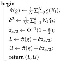
Section 3 presents the proposed approach.
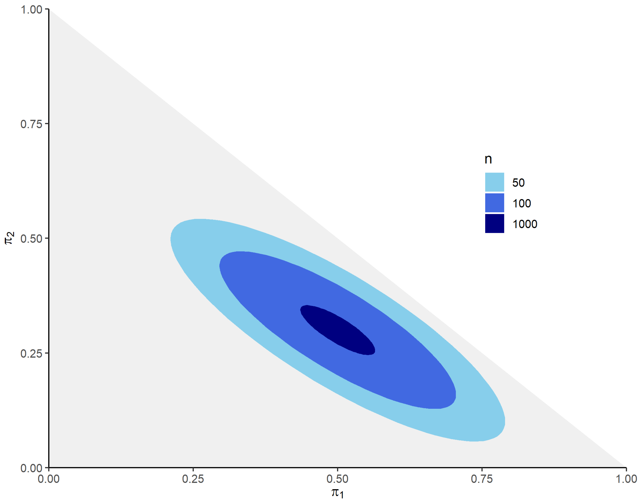
Section 4 illustrates the proposed approach with examples and presents numerical experiments to analyze the coverage characteristics of the approach.
Section 5 concludes this work and discusses potential future directions of research.
2. Results Underpinning the Proposed Approach and Proofs
2.1. Results Underpinning the Proposed Approach
Let be an irreducible Markov chain with finite and discrete state-space . Throughout this paper, for any integer n we denote as the set of indices from 1 to n. Let P be the transition matrix, and assume that P admits the unique stationary distribution vector .
Let be based on a sample path of this Markov chain, and let be the maximum likelihood estimate of P based on this sample path. Assume that admits the unique stationary distribution vector . Furthermore, , let . Assume that , .
Theorem 1. andwhere is a symmetric matrix that depends on the kth row of ; is a column vector that depends on the column of a one-condition g-inverse of ; and , The definition of a one-condition g-inverse is given in
Section 2.2. We then expose the proof of Theorem 1 in
Section 2.3. The proof of Equation (
3) is similar to that of Theorem 3.1 in [
11]. The key difference between Equation (
3) and Theorem 3.1 in [
11] is that Equation (3) only involves inputs that can be inferred from
.
2.2. Core Concepts Underlying the Proof of Theorem 1
The following definition and Equation (
4) are drawn from [
19].
Definition 1 (One-condition g-inverse). A one-condition g-inverse (or one-condition generalized inverse) of a matrix A is any matrix such that
Let
be the transition matrix of a finite irreducible Markov chain, which is assumed to have the associated steady-state distribution vector
. Let
be the transition matrix of the perturbed Markov chain, where
is the matrix of perturbations. Notice that
, and
.
is assumed to admit the unique steady-state distribution vector
. Then, according to Theorem 2.1 in [
19],
where
,
,
I is the identity matrix, and
G is a one-condition g-inverse of
.
An exhaustive review of the different ways to compute matrix
G (and therefore matrix
H) is beyond the scope of this work. For the purposes of the examples in
Section 4, we computed
G as the so-called group inverse (see [
20]) of
. This choice is mainly motivated by ease of computation for the transition matrix of an ergodic Markov chain (Theorem 5.2 in [
20]). Indeed, the most computationally intensive step is the calculation of the inverse of a
principal submatrix of
.
It bears mentioning that
H can also be derived based on the matrix of mean first passage times and the steady-state distribution vector (see [
19]), which can enhance interpretability.
For a sample path of length N characterized by the sequence of observed states of a discrete ergodic Markov chain with transition matrix P, let . For any pair of states , let be the number of transitions from to in the sample path , or more formally . We will refer to as the sequence matrix. Also, throughout this work, we will assume that .
Lemma 1. Conditional on , the rows of M are mutually independent and respectively follow multinomial distributions with trials and unknown event probabilities .
Proof. Conditional on , the joint outcome of can be equated to independent trials (independence follows from the Markov property) where the outcome of each trial has a categorical distribution with fixed success probabilities . In other words, conditional on , jointly follow a multinomial distribution with trials and event probabilities .
Also, for
let
be a vector corresponding to row
i of the sequence matrix M and let
be a vector corresponding to row
i of the unknown transition matrix
P. Given known
and unknown
, for
:
□
Importantly, independence between the rows only holds conditional on the knowledge of . Otherwise, the rows of M are of course not independent since crucially depends on .
2.3. Proof of Theorem 1
Notice that for a sample path of an irreducible Markov chain with discrete and finite state-space , transition matrix P, and unique steady-state distribution vector , we can build the maximum likelihood estimate of P based on the sequence matrix. Moreover, can be viewed as a perturbation of P (and vice versa).
Assume that admits the unique steady-state distribution vector . Let and , where , I is the identity matrix, and G is a one-condition g-inverse of . In this context, the following lemmas apply.
Proof. By matrix multiplication and following Equation (
4),
Hence,
The second equality follows from conditional independence between the rows of the sequence matrix (Lemma 1). □
The following three lemmas are corollaries of Lemmas 3.4–3.6 in [
11], except that here
and
, whereby
,
I is the identity matrix, and
G is a one-condition g-inverse of
. For the sake of brevity, we refer the reader to [
11] for the respective proofs.
Lemma 5. Without a loss of generality, assume that the row vector has only nonzero elements. ,whereand Notice that
From these equalities and Lemma 5
and
Additionally, given Lemmas 2 and 4, respectively,
and
which proves Theorem 1.
5. Conclusions
In this paper, we proposed a method to numerically determine confidence regions for the steady-state probabilities and confidence intervals for additive functionals of an ergodic finite-state Markov chain. The novelty of our method stems from the fact that it simultaneously fulfills three conditions. First, our method is asymptotically exact. Second, our method requires only a single sample path as an input. Third, our method does not require any inputs beyond what can be inferred from . To the best of our knowledge, no method that satisfies all three conditions has previously been proposed in the literature.
Since our method relies on asymptotically exact results, we expect it to work well for large enough values of
N, as exemplified by the numerical experiment in
Section 4.2. However, since the premise of this paper is that nothing is known about the Markov chain beyond what can be inferred from
, what constitutes a large enough value of
N cannot be known with certainty. If
N is too small, the variance estimate
may become numerically unstable, as illustrated in
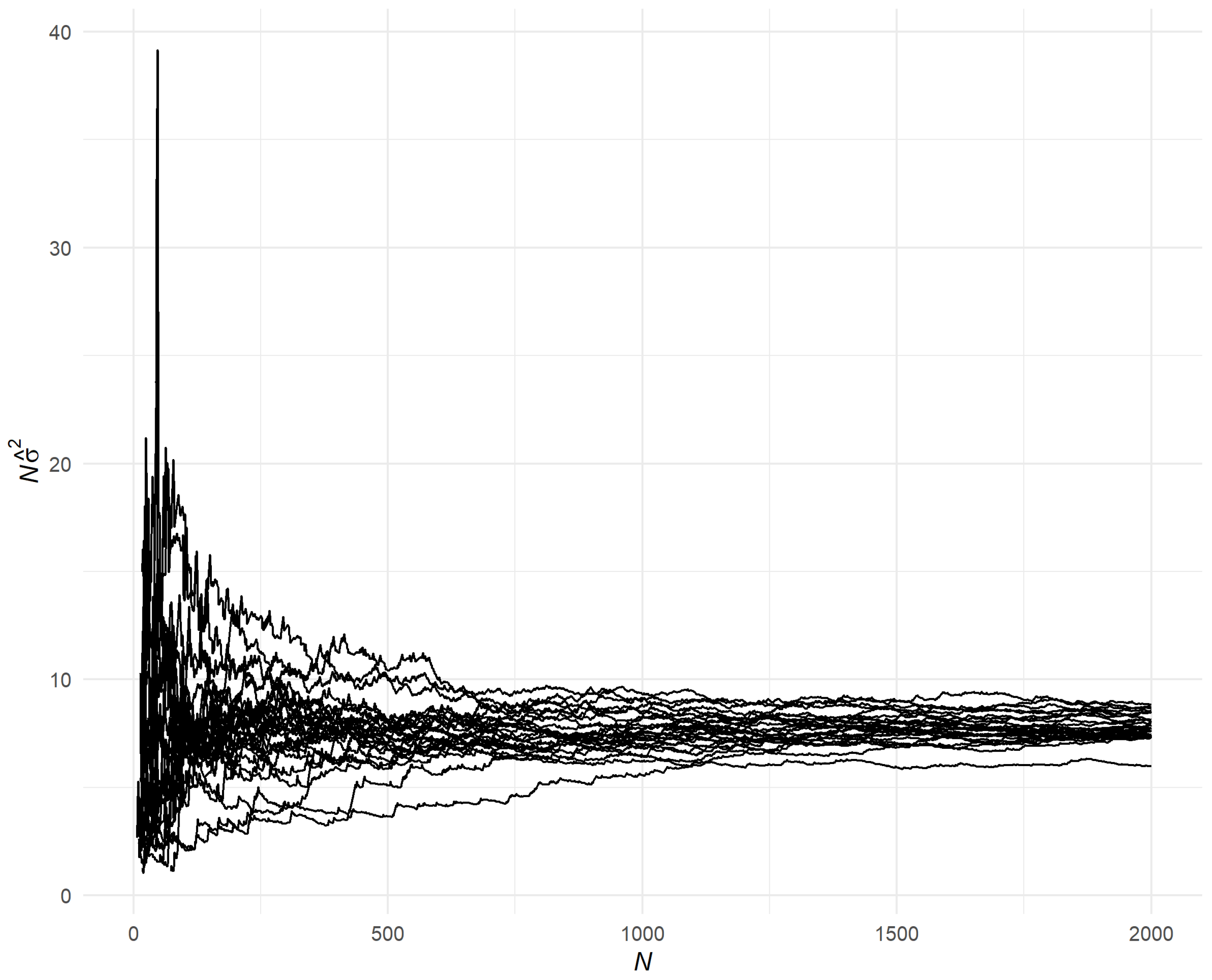
Section 4.2. In this case, the confidence interval’s realized coverage level could undershoot the desired confidence level. One way to mitigate this risk could be to analyze the convergence of
as
N is increased to include the entire sample path (see
Section 4.2 and in particular
Figure 2).
Another aspect to consider is bias, which could be a potential concern for small values of
N. In order for the confidence intervals discussed in
Section 3 to be valid, we need to be able to assume that
(or at least that
). This is not a strong assumption for large
N since
is an unbiased estimator of
, assuming the initial state is sampled from
. However, given the premise that nothing is known beyond what can be inferred from
, it may be difficult to determine with certainty whether
is large enough to make this assumption. One way to address this issue could be through the lens of mixing time (see [
12] for more details). If
N exceeds the mixing time, then bias is likely close to 0. An approach to estimating mixing time based on a single sample path was proposed in [
24].
Lastly, an open question is how one might extend our proposed approach to infinite state-space Markov chains.


