Generalized Laplace Transform with Adomian Decomposition Method for Solving Fractional Differential Equations Involving ψ-Caputo Derivative

Abstract

In this study, we introduced the $\psi$-Laplace transform Adomian decomposition method, which is a combination of the efficient Adomian decomposition method with the generalization of the classical Laplace transform to treat fractional differential equations with respect to another function, $\psi$, in the Caputo sense. To validate the effectiveness of this method, we applied the derived recurrent scheme of the $\psi$-Laplace Adomian decomposition on several test numerical problems, including a real-life scenario in pharmacokinetics that models the movement of drug concentration in human blood. The solutions obtained closely matched the known solutions for the test problems. Additionally, in the pharmacokinetics case, the results were consistent with the available physical data. Consequently, this method simplifies the verification of numerous related aspects and proves advantageous in solving various $\psi$-fractional differential equations.

1. Introduction

The field of fractional-order calculus focuses on the analysis and investigation of derivatives and integrals of non-integer orders. In addition, the area has recently seen increasing advancements with immense relevance in various fields of contemporary applications, like control theory, fluid flow, probability theory, thermodynamics, and dynamical systems [1,2]. Furthermore, the field of fractional calculus is multidirectional, as it lacks a unique definition compared to classical calculus, which follows a single approach. Different definitions of fractional derivatives exist, such as Riemann–Liouville, Caputo, Hadamard, Erdelyi–Kober, Riesz, Hilfer, and Atangana–Baleanu. The history of this topic is available in [3,4,5]. Several studies have investigated the application of different types of fractional derivatives to handle various classes of fractional differential equations (FDEs). These studies highlight the versatility of fractional calculus in modeling complex phenomena across multiple fields.

A new version of the fractional derivative was proposed by Almeida [6]. The $\psi$-Caputo fractional derivative generalizes various other formulations of fractional derivatives, such as the Caputo and Hadamard ones. Various types of fixed-point theorems are currently used as essential tools to demonstrate the existence and uniqueness of solutions for diverse classes of $\psi$-fractional differential equations ($\psi$-FDEs) [7,8,9,10]. Recently, the field of fractional calculus has grown to encompass numerous novel fractional integral and derivative operators. Generally, the introduction of a new fractional derivative arises from one of two motives: either to represent physical phenomena that current fractional derivatives cannot adequately describe or to incorporate specific mathematical characteristics absent from existing fractional derivatives. In addition, recent studies on the $\psi$-Caputo differential operators suggest that $\psi$-FDEs offer greater flexibility and yield appropriate results in various scenarios. Almeida, in a study focusing on world population growth, employed the $\psi$-Caputo derivative and showcased that the model’s accuracy relies on carefully choosing the fractional operator. Additionally, opting for a suitable trial function is vital for accurately representing physical phenomena and improves the practical applicability of the approach from a standpoint [7,11]. Currently, it is noted that $\psi$-FDEs do not realize analytical solutions; approximation methods, including semi-analytical methods, will be suitable tools for their analysis. The literature presents various methods for the acquisition of both the analytical and computation solutions of the initial value problem (IVP) for $\psi$-FDEs, such as the $\psi$-Haar wavelet method [12], and the operational matrix by introducing the $\psi$-shifted Legendre polynomial [13]. Developing appropriate techniques to derive analytical and numerical solutions for specific classes of $\psi$-FDEs is among the taxing challenges in the area of fractional calculus. Thus, in recent years, various scientists have shown interest in devising new analytical and numerical methods to tackle the blazing occurrence of complex physical phenomena. In this regard, this discussion will focus on the generalized Laplace transform introduced by [14], referred to as the $\psi$-Laplace transform ($\psi$-LT). This operator smoothly integrates with fractional derivatives and integrals involving functions [15] for some special applications on certain differential equations.

Furthermore, the Adomian decomposition method (ADM) is a semi-analytical technique that has proven highly effective for solving a wide range of FDEs. It finds significant applications in various domains of the life sciences. Notably, ADM requires less effort than many established methods, making it a practical choice. This method reduces the computational workload. The decomposition process in Adomian’s method is achieved effortlessly without linearizing the given problem.

ADM has proven to be a powerful tool for solving various FDEs. Its applications include analyzing relaxation-oscillation differential equations using the $\psi$-Caputo derivative [16] and studying generalized fractional Riccati differential equations with respect to another function, $\psi$ [17]. To enhance accuracy and efficiency, ADM has undergone several modifications aimed at improving convergence speed and reducing computational time. These advancements have led to significant progress, resulting in the faster convergence of series solutions compared to the standard ADM. The modified ADM has demonstrated computational efficiency across various models, making it invaluable for researchers in applied science. Recently, an efficient modification [18] was introduced to solve nonlinear FDEs. Additionally, researchers have integrated ADM with various integral transformations, such as Laplace, Sumudu, Natural, and Elzaki transforms. These combinations have proven effective in solving different FDEs models. By utilizing the decomposition technique instead of standard procedures for obtaining accurate solutions, the coupling of the Laplace transform with the Adomian decomposition method leads to the Laplace–Adomian decomposition method (LADM). This efficient approach continues to be widely used in various types of FDEs, which model a broad range of applications in science and engineering [19,20].

Motivated by the need to expand the applicability of recently proposed $\psi$-fractional definitions to more realistic scientific scenarios, this paper aims to apply the standard ADM alongside the generalized Laplace transform ($\psi$-LADM) to address a class of FDEs that incorporate $\psi$-Caputo fractional derivatives, $\psi$-FDEs. The generalized $\psi$-LADM recurrent scheme derived through this approach will be evaluated with several test numerical problems, including a real-life application in pharmacokinetics. We selected the $\psi$-LADM method due to its promising results in the numerical examples discussed later in the paper. Compared to previous studies on $\psi$-FDEs, our findings demonstrate greater accuracy. The authors in [21] used the same technique to solve a system of $\psi$-FDEs and achieved excellent results, showing that this method can effectively solve different types of $\psi$-FDEs. Although we encountered some difficulty in obtaining the inverse $\psi$-Laplace transform for certain functions, the method provided excellent results and was easier to implement in mathematical software, specifically Maple 22, as used in this study. We hope that our research will provide future researchers with a broader selection of methods for solving various types of problems.

Moreover, the structure of the current manuscript is as follows: Section 2 presents some related definitions and theorems, Section 3 derives the general $\psi$-LADM scheme, Section 4 demonstrates the beseeched methodology on test problems, including a physical scenario in pharmacokinetics, while Section 5 gives some concluding notes.

2. Preliminaries

In this section, we introduce essential definitions of $\psi$-fractional operators and explore their fundamental properties. Additionally, we discuss a generalized $\psi$-Laplace Transform ($\psi$-LT), the $\psi$-LT of some elementary functions, and the $\psi$-LT for $\psi$-fractional operators and various special functions that are crucial for finding solutions to $\psi$-fractional differential equations ($\psi$-FDEs).

Definition 1. 

The fractional integral of order $\alpha >0$ for a function y with respect to another function ψ is given by the following expression [6]. Here, $y:I\to \mathbb{R}$ is an integrable function, $I=[a,b]$, $\alpha \in \mathbb{R}$, $n\in \mathbb{N}$, and $\psi \left(x\right)\in C^n\left(I\right)$ is a function such that ${\psi }^{\prime }\left(x\right)\ne 0$ for all $x\in I$.

$$I_a^{\alpha ,\psi }y\left(x\right):={\left\{\Gamma \left(\alpha \right)\right\}}^{-1}{\int }_a^x{\psi }^{\prime }\left(t\right){(\psi \left(x\right)-\psi \left(t\right))}^{-1+\alpha }y\left(t\right)dt,$$

(1)

In this context, Γ represents the gamma function. It is important to note that Equation (1) is simplified to the Riemann–Liouville and Hadamard fractional integrals when $\psi \left(x\right)=x$ and $\psi \left(x\right)=ln\left(x\right)$, respectively.

Definition 2. 

Consider a function $y:I\to \mathbb{R}$ defined on the interval $I=[a,b]$, where y is integrable. For a fractional order $\alpha >0$ and a function $\psi \in C^n\left(I\right)$ such that ${\psi }^{\prime }\left(x\right)\ne 0$ for all $x\in I$, the fractional derivative of y with respect to ψ is defined as follows [6]:

$$\begin{array}{cc}\hfill D_{a^{+}}^{\alpha ,\psi }y\left(x\right)& :={\left({\displaystyle \frac{1}{{\psi }^{\prime }\left(x\right)}}{\displaystyle \frac{d}{dx}}\right)}^n{I}_{a^{+}}^{n-\alpha ,\psi }y\left(x\right),\hfill \end{array}$$

(2)

$$\begin{array}{cc}\hfill & ={\left\{\Gamma (n-\alpha )\right\}}^{-1}{\left({\displaystyle \frac{1}{{\psi }^{\prime }\left(x\right)}}{\displaystyle \frac{d}{dx}}\right)}^n{\int }_a^x{\psi }^{\prime }\left(t\right){(\psi \left(x\right)-\psi \left(t\right))}^{-1-\alpha +n}y\left(t\right)dt,\hfill \end{array}$$

(3)

where $n=1+\lfloor \alpha \rfloor$.

Note that Equation (2) is reduced to the Riemann–Liouville and Hadamard fractional derivatives when $\psi \left(x\right)=x$ and $\psi \left(x\right)=ln\left(x\right)$, respectively.

Definition 3. 

Consider the interval $I=[a,b]$, where $\alpha >0$ and $n\in \mathbb{N}$. Let ψ and y be two functions in $C^n\left(I\right)$, with ψ being an increasing function and ${\psi }^{\prime }\left(x\right)\ne 0$ for all $x\in I$. The ψ-Caputo fractional derivative of order α for the function y is defined as follows [6]:

$${}^{C}D_a^{\alpha ,\psi }y\left(x\right)=I_a^{n-\alpha ,\psi }{\left({\displaystyle \frac{1}{{\psi }^{\prime }\left(x\right)}}{\displaystyle \frac{d}{dx}}\right)}^{n}y\left(x\right),$$

(4)

where $n=1+\lfloor \alpha \rfloor$ if $\alpha \notin \mathbb{N}$, and $n=\alpha$ if $\alpha \in \mathbb{N}$. To simplify notation, we will use the shorthand symbol

$$\begin{array}{c}\hfill y_{\psi }^{\left[n\right]}\left(x\right):={\left({\displaystyle \frac{1}{{\psi }^{\prime }\left(x\right)}}{\displaystyle \frac{d}{dx}}\right)}^{n}y\left(x\right).\end{array}$$

From the definition, it follows that

$${}^{C}D_a^{\alpha ,\psi }y\left(x\right)=\left\{\begin{array}{cc}{\left\{\Gamma (n-\alpha )\right\}}^{-1}{\int }_a^x{\psi }^{\prime }\left(t\right){(\psi \left(x\right)-\psi \left(t\right))}^{n-\alpha -1}{y}_{\psi }^{\left[n\right]}\left(t\right)dt,\hfill & \mathit{if}\alpha \notin \mathbb{N},\hfill \\ y_{\psi }^{\left[n\right]}\left(x\right),\hfill & \mathit{if}\alpha \in \mathbb{N}.\hfill \end{array}\right.$$

(5)

Note that Equation (5) is reduced to the classical Caputo derivative and the Caputo–Hadamard fractional derivative when $\psi \left(x\right)=x$ and $\psi \left(x\right)=ln\left(x\right)$, respectively.

Additionally, by considering $y\left(x\right)={(\psi \left(x\right)-\psi \left(a\right))}^{\beta -1}$, where $\beta \in \mathbb{R}$ with $\beta >n$ and $\alpha >0$, the following key properties of $\psi \left(x\right)$-fractional operators are derived [6]:

• ${}^{C}D_{a^{+}}^{\alpha ,\psi }y\left(x\right)={\displaystyle \frac{\Gamma \left(\beta \right)}{\Gamma (\beta -\alpha )}}{(\psi \left(x\right)-\psi \left(a\right))}^{\beta -\alpha -1}$;
• $I_a^{\alpha ,\psi }y\left(x\right)={\displaystyle \frac{\Gamma \left(\beta \right)}{\Gamma (\beta +\alpha )}}{(\psi \left(x\right)-\psi \left(a\right))}^{\beta +\alpha -1}$;
• $I_a^{\alpha ,\psi }\left({}^{C}D_a^{\alpha ,\psi }y\left(x\right)\right)=y\left(x\right)-{\sum }_{k=0}^{n-1}{\displaystyle \frac{y_{\psi }^{\left[k\right]}\left(a\right)}{k!}}{(\psi \left(x\right)-\psi \left(a\right))}^k$.
  Furthermore, when $\alpha \in (0,1)$, this is simplified to $I_a^{\alpha ,\psi }\left({}^{C}D_a^{\alpha ,\psi }y\left(x\right)\right)=y\left(x\right)-y\left(a\right)$.

Furthermore, several specialized functions are particularly useful for solving $\psi$-FDEs. In the following definitions and theorems, we introduce a selection of these functions.

Definition 4. 

The Mittag-Leffler function $E_{\alpha }\left(z\right)$ is a well-known function in the theory of fractional calculus, introduced by Gösta Mittag-Leffler. It is expressed as follows [15]:

$$E_{\alpha }\left(z\right)=\sum _{k=0}^{\infty }{\displaystyle \frac{z^k}{\Gamma (\alpha k+1)}},\alpha \in \mathbb{C},\mathrm{Re}\left(\alpha \right)>0.$$

(6)

Additionally, Wiman generalized the Mittag-Leffler function to a two-parameter form, given by:

$$E_{\alpha ,\beta }\left(z\right)=\sum _{k=0}^{\infty }{\displaystyle \frac{z^k}{\Gamma (\alpha k+\beta )}},\alpha ,\beta \in \mathbb{C},\mathrm{Re}\left(\alpha \right)>0.$$

(7)

In a similar vein, Prabhakar introduced an even more general form, known as the three-parameter Mittag-Leffler function or Prabhakar function, defined as:

$$E_{\alpha ,\beta }^{\chi }\left(z\right):={\displaystyle \frac{1}{\Gamma \left(\chi \right)}}\sum _{k=0}^{\infty }{\displaystyle \frac{z^k\Gamma (\chi +k)}{k!\Gamma (\alpha k+\beta )}},\alpha ,\beta ,\chi \in \mathbb{C},\mathrm{Re}\left(\alpha \right)>0.$$

(8)

Definition 5. 

If $y:[0,\infty )\to \mathbb{R}$ is a real-valued function and ψ is an increasing positive function with $\psi \left(0\right)=0$, then the Laplace transform of the function y with respect to the function ψ is defined as follows [14,15]:

$${\mathcal{L}}_{\psi }\left\{y\left(x\right)\right\}=Y\left(s\right)={\int }_0^{\infty }{e}^{-s\psi \left(x\right)}{\psi }^{\prime }\left(x\right)y\left(x\right)dx,\forall s\in \mathbb{C}.$$

(9)

Theorem 1. 

The generalized Laplace transform can be expressed as a combination of the classical Laplace transform and the operation of composition with ψ or ${\psi }^{-1}$, as shown below:

$${\mathcal{L}}_{\psi }=\mathcal{L}\circ {\phi }_{\psi }^{-1},$$

(10)

where the functional operator ${\phi }_{\psi }$ is defined by

$$\left({\phi }_{\psi }f\right)\left(x\right)=f\left(\psi \left(x\right)\right).$$

(11)

Corollary 1. 

The inverse generalized Laplace transform can be expressed as a combination of the inverse classical Laplace transform and the operation of composition with ψ or ${\psi }^{-1}$, as described below:

$${\mathcal{L}}_{\psi }^{-1}={\phi }_{\psi }\circ {\mathcal{L}}^{-1},$$

(12)

or, in other words,

$${\mathcal{L}}_{\psi }^{-1}\left[Y\left(s\right)\right]={\displaystyle \frac{1}{2\pi i}}{\int }_{c-i\infty }^{c+i\infty }{e}^{s\psi \left(t\right)}Y\left(s\right)ds.$$

(13)

To calculate the generalized Laplace transform of various elementary functions, consult

Table 1. $\psi$-Laplace transform of some functions.

$y\left(x\right)$	${\mathcal{L}}_{\psi }\left\{y\left(x\right)\right\}=Y\left(s\right)$
1	${\displaystyle \frac{1}{s}},s>0$
$e^{a\psi \left(x\right)}$	${\displaystyle \frac{1}{s-a}}$ for $s>a$
${\left(\psi \left(x\right)\right)}^{\alpha }$	${\displaystyle \frac{\Gamma (\alpha +1)}{s^{\alpha +1}}},$ for $s>0$
$E_{\alpha }\left(\lambda {\left(\psi \left(x\right)\right)}^{\alpha }\right)$	${\displaystyle \frac{s^{\alpha -1}}{s^{\alpha }-\lambda }},$ for $\mathrm{Re}\left(\alpha \right)>0,$ and $\left|{\displaystyle \frac{\lambda }{s^{\alpha }}}\right|<1$
${\left(\psi \left(x\right)\right)}^{\alpha -1}{E}_{\alpha ,\alpha }\left(\lambda {\left(\psi \left(x\right)\right)}^{\alpha }\right)$	${\displaystyle \frac{1}{s^{\alpha }-\lambda }}$ for $\mathrm{Re}\left(\alpha \right)>0,$ and $\left|{\displaystyle \frac{\lambda }{s^{\alpha }}}\right|<1$
${\left(\psi \left(x\right)\right)}^{\beta -1}{E}_{\alpha ,\beta }^{\gamma }\left(\lambda {\left(\psi \left(x\right)\right)}^{\alpha }\right)$	${\displaystyle \frac{s^{\alpha \gamma -\beta }}{{(s^{\alpha }-\lambda )}^{\gamma }}}$ for $\mathrm{Re}\left(\alpha \right)>0,$ and $\left|{\displaystyle \frac{\lambda }{s^{\alpha }}}\right|<1$

.

Theorem 2. 

Let y be a piecewise continuous function of ψ-exponential order, defined over each finite interval. Then, for any $\alpha >0$,

$${\mathcal{L}}_{\psi }\left\{I_0^{\alpha ,\psi \left(x\right)}y\left(x\right)\right\}=s^{-\alpha }{\mathcal{L}}_{\psi }\left\{y\left(x\right)\right\}.$$

(14)

Theorem 3. 

Assume $\alpha >0$, $n=\lfloor \alpha \rfloor +1$, and let y be a function such that $y\left(x\right)$, $I_0^{n-\alpha ,\psi \left(x\right)}y\left(x\right)$, $D_0^{1,\psi \left(x\right)}{I}_0^{n-\alpha ,\psi \left(x\right)}y\left(x\right)$,…, $D_0^{n,\psi \left(x\right)}{I}_0^{n-\alpha ,\psi \left(x\right)}y\left(x\right)$ are of ψ-exponential order and continuous over the interval $(0,\infty )$. Additionally, assume ${}^{R}D_0^{\alpha ,\psi \left(x\right)}y\left(x\right)$ is piecewise continuous over the interval $[0,\infty )$. Then,

$${\mathcal{L}}_{\psi }\left\{{}^{R}D_0^{\alpha ,\psi \left(x\right)}y\left(x\right)\right\}=s^{\alpha }{\mathcal{L}}_{\psi }\left\{y\left(x\right)\right\}-\sum _{i=0}^{n-1}{s}^{n-1-i}\left(I_0^{n-i-\alpha ,\psi \left(x\right)}y\right)\left(0\right).$$

(15)

Theorem 4. 

Assume $\alpha >0$, $n=\lfloor \alpha \rfloor +1$, and let y be a function such that $y\left(x\right)$, ${}^{C}D_0^{1,\psi \left(x\right)}y\left(x\right)$, ${}^{C}D_0^{2,\psi \left(x\right)}y\left(x\right)$,…, ${}^{C}D_0^{n-1,\psi \left(x\right)}y\left(x\right)$ are of ψ-exponential order and continuous over the interval $[0,\infty )$. Additionally, assume ${}^{C}D_0^{\alpha ,\psi \left(x\right)}y\left(x\right)$ is piecewise continuous over the interval $[0,\infty )$. Then,

$${\mathcal{L}}_{\psi }\left\{{}^{C}D_0^{\alpha ,\psi \left(x\right)}y\left(x\right)\right\}=s^{\alpha }{\mathcal{L}}_{\psi }\left\{y\left(x\right)\right\}-\sum _{i=0}^{n-1}{s}^{\alpha -1-i}\left(D_0^{i,\psi \left(x\right)}y\right)\left(0\right).$$

(16)

3. Fundamental Description of $\mathbf{\psi }$-LADM for Solving $\mathbf{\psi }$-FDEs

In the present section, we will utilize the $\psi$-LADM for solving IVPs of $\psi$-FDEs involving $\psi$-Caputo derivatives.

Thus, in presenting the methodology, we consider a generalized IVP for FDEs amidst any arbitrary function $\psi$ as follows

$${}^{C}D_{a^{+}}^{\alpha ,\psi }y\left(x\right)=f(x,y\left(x\right)),x\in [a,b],$$

(17)

and constrained by the following initial conditions

$$y\left(a\right)=y_a,\mathrm{and}{y}_{\psi }^{\left[k\right]}\left(a\right)=y_a^k,k=1,2,\cdots ,n-1,$$

(18)

where ${}^{C}D_{a^{+}}^{\alpha ,\psi }$ denotes the $\psi$-Caputo fractional operator of order $\alpha ,$$\psi$ is any arbitrary function, and $y\left(x\right)$ is the solution to be known, while $f(x,y(x\left)\right)$ is an arbitrary continuous nonlinear function.

To solve the problem expressed in (17) by $\psi$-LADM, we operate $\psi$-LT on both sides to obtain

$${\mathcal{L}}_{\psi }{\{}^C{D}_{a^{+}}^{\alpha ,\psi \left(x\right)}y\left(x\right)\}={\mathcal{L}}_{\psi }\left\{f(x,y\left(x\right))\right\}.$$

(19)

Further, on using (16) together with the prescribed initial conditions, one obtains

$$s^{\alpha }{\mathcal{L}}_{\psi }\left\{y\left(x\right)\right\}-\sum _{k=0}^{n-1}{s}^{\alpha -1-k}{y}_{\psi }^{\left[k\right]}\left(a\right)={\mathcal{L}}_{\psi }\left\{f(x,y\left(x\right))\right\},$$

(20)

$${\mathcal{L}}_{\psi }\left\{y\left(x\right)\right\}-\sum _{k=0}^{n-1}{\displaystyle \frac{1}{s^{k+1}}}{y}_{\psi }^{\left[k\right]}\left(a\right)={\displaystyle \frac{1}{s^{\alpha }}}{\mathcal{L}}_{\psi }\left\{f(x,y\left(x\right))\right\}.$$

(21)

Next, applying the inverse $\psi$-LT on both sides of the latter equation, we obtain

$${\mathcal{L}}_{\psi }^{-1}\left\{{\mathcal{L}}_{\psi }\left\{y\left(x\right)\right\}\right\}-{\mathcal{L}}_{\psi }^{-1}\left\{\sum _{k=0}^{n-1}{\displaystyle \frac{1}{s^{k+1}}}{y}_{\psi }^{\left[k\right]}\left(a\right)\right\}={\mathcal{L}}_{\psi }^{-1}\left\{{\displaystyle \frac{1}{s^{\alpha }}}{\mathcal{L}}_{\psi }\left\{f(x,y\left(x\right))\right\}\right\},$$

(22)

$$y\left(x\right)={\mathcal{L}}_{\psi }^{-1}\left\{\sum _{k=0}^{n-1}{\displaystyle \frac{1}{s^{k+1}}}{y}_{\psi }^{\left[k\right]}\left(a\right)\right\}+{\mathcal{L}}_{\psi }^{-1}\left\{{\displaystyle \frac{1}{s^{\alpha }}}{\mathcal{L}}_{\psi }\left\{f(x,y\left(x\right))\right\}\right\}.$$

(23)

Further, the standard ADM defines the solution $y\left(x\right)$ by the following infinite series

$$y\left(x\right)=\sum _{n=0}^{\infty }{y}_n\left(x\right).$$

(24)

On the other hand, the nonlinear term is expressed through the decomposed series of Adomian polynomials $A_n$ as follows

$$f(x,y\left(x\right))=\sum _{n=0}^{\infty }{A}_n.$$

(25)

where $A_n$ are unequivocally expressed as follows

$$A_n={\displaystyle \frac{1}{n!}}{\displaystyle \frac{d^n}{d{\lambda }^n}}{\left[N\left(\sum _{i=0}^{\infty }{\lambda }^i{y}_i\right)\right]}_{\lambda =0},n=0,1,2,\cdots$$

(26)

Therefore, with the above-decomposed series, Equation (23) is thus re-expressed as follows

$$\sum _{n=0}^{\infty }{y}_n\left(x\right)={\mathcal{L}}_{\psi }^{-1}\left\{\sum _{k=0}^{n-1}{\displaystyle \frac{1}{s^{k+1}}}{y}_{\psi }^{\left[k\right]}\left(a\right)\right\}+{\mathcal{L}}_{\psi }^{-1}\left\{{\displaystyle \frac{1}{s^{\alpha }}}{\mathcal{L}}_{\psi }\left\{\sum _{n=0}^{\infty }{A}_n\right\}\right\},$$

(27)

upon which the formal recursive relation is acquired as follows

$$\left\{\begin{array}{c}{y}_0\left(x\right)={\mathcal{L}}_{\psi }^{-1}\left\{\sum _{k=0}^{n-1}{\displaystyle \frac{1}{s^{k+1}}}{y}_{\psi }^{\left[k\right]}\left(a\right)\right\},\hfill \\ y_n\left(x\right)={\mathcal{L}}_{\psi }^{-1}\left\{{\displaystyle \frac{1}{s^{\alpha }}}{\mathcal{L}}_{\psi }\left\{A_{n-1}\right\}\right\},n\ge 1.\hfill \end{array}\right.$$

(28)

Finally, a realistic solution is obtained by considering the following m-term approximations

$${\varphi }_n\left(x\right)=\sum _{i=0}^{n-1}{y}_i\left(x\right),$$

(29)

with the closed-from solution taking the following form:

$$y\left(x\right)=\underset{n\to \infty }{lim}{\varphi }_n\left(x\right)=\sum _{i=0}^{\infty }{y}_i\left(x\right).$$

(30)

4. Applications

The current section assesses the competency of the proposed $\psi$-LADM scheme on some test problems. More importantly, the section considers both nonlinear and linear $\psi$-FDEs, including a real-life scenario concerning the field of pharmacokinetics, where a mathematical model for the variation of drug concentration in human blood is analyzed.

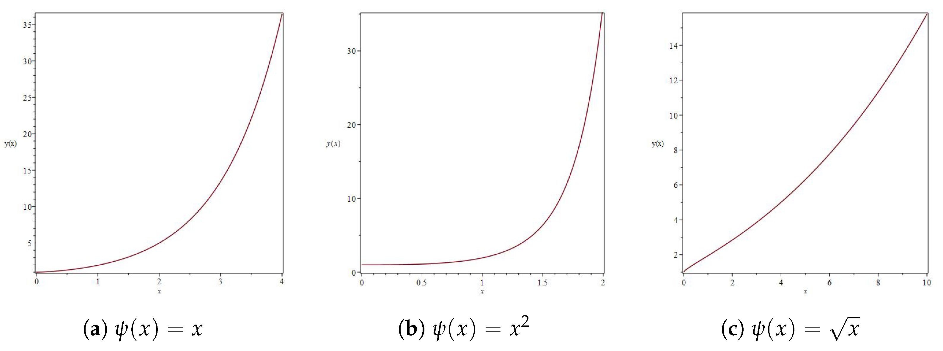
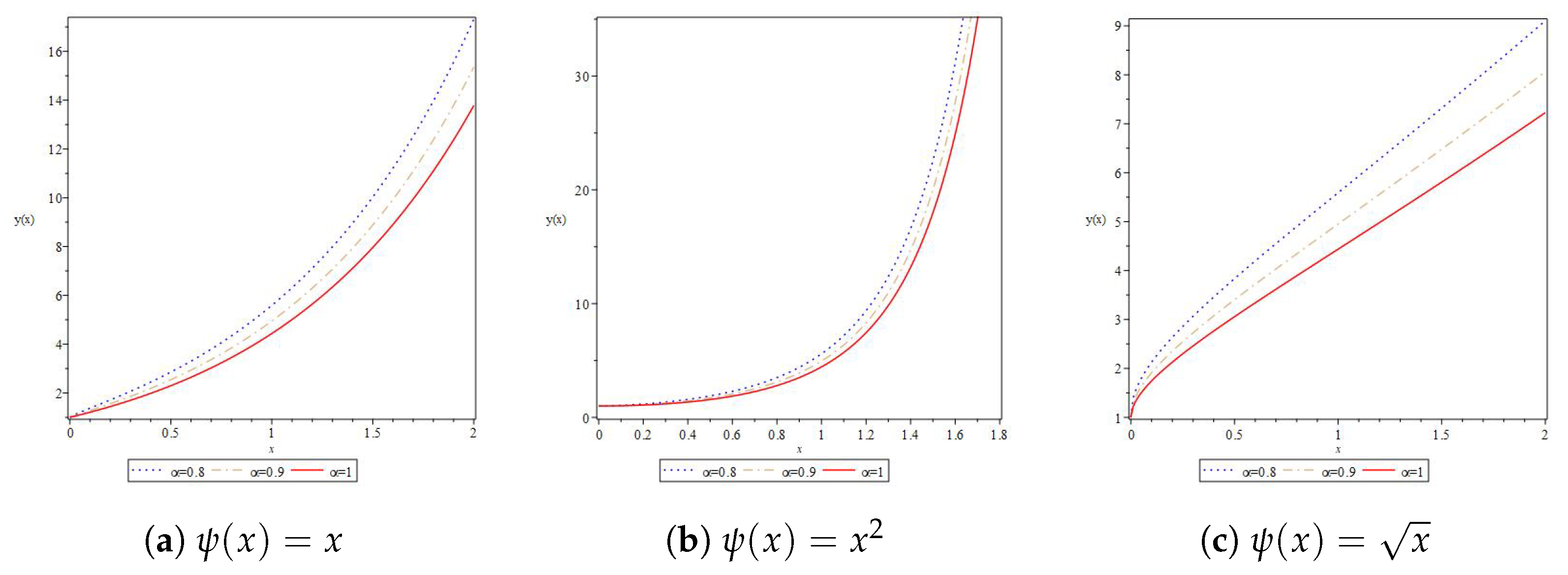
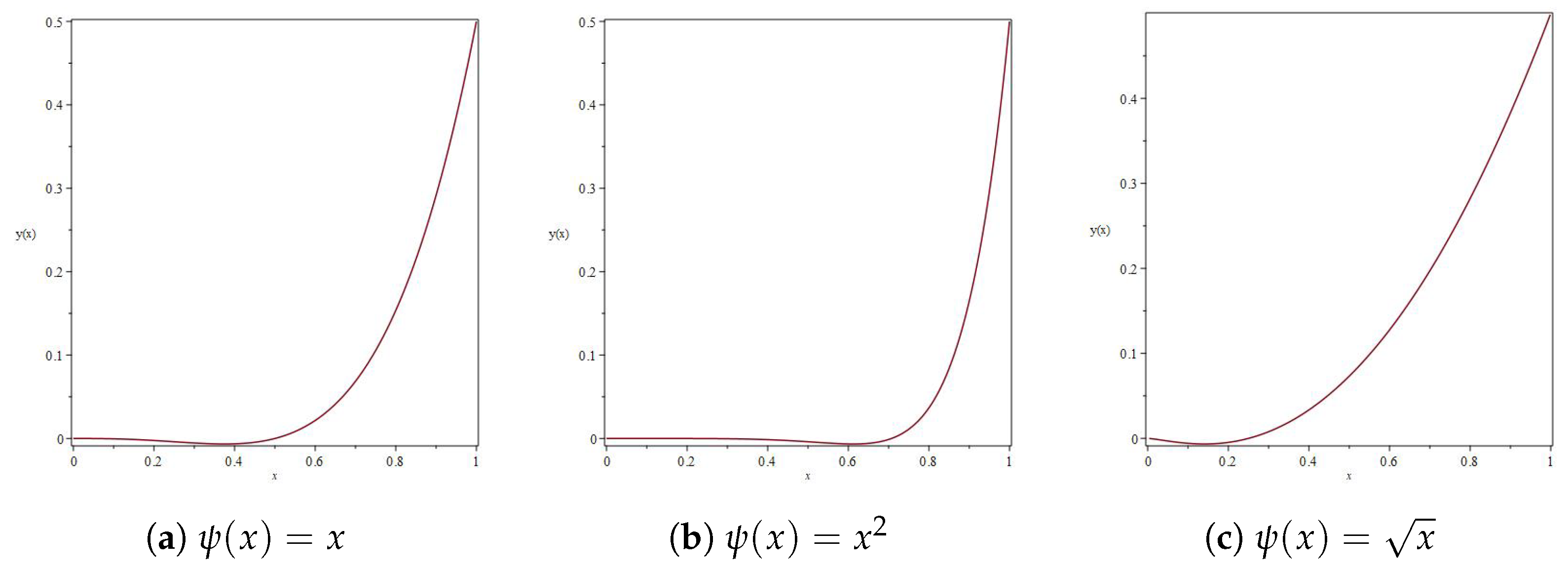
4.1. Numerical Applications

In this subsection, some interesting $\psi$-FDEs are offered as numerical examples and further analyzed using the $\psi$-LADM approach. Indeed, both the nonlinear and linear IVP featuring $\psi$-fractional derivatives are considered.

Example 1. 

Consider the IVP for ψ-FDE as follows [7]

$$\begin{array}{c}\hfill {}^{C}D_{0^{+}}^{3/2,\psi \left(x\right)}y\left(x\right)=y\left(x\right),\\ \hfill y\left(0\right)=1,y_{\psi }^{\left[1\right]}\left(0\right)=0.\end{array}$$

(31)

To solve (31) by ψ-LADM, we apply ψ-LT on both sides of the equation, which when using (16) gives

$${\mathcal{L}}_{\psi }\left\{{}^{C}D_{0^{+}}^{3/2,\psi \left(x\right)}y\left(x\right)\right\}={\mathcal{L}}_{\psi }\left\{y\left(x\right)\right\},$$

(32)

$$s^{3/2}{\mathcal{L}}_{\psi }\left\{y\left(x\right)\right\}-s^{1/2}y\left(0\right)={\mathcal{L}}_{\psi }\left\{y\left(x\right)\right\},$$

$${\mathcal{L}}_{\psi }\left\{y\left(x\right)\right\}-{\displaystyle \frac{1}{s}}={\displaystyle \frac{1}{s^{3/2}}}{\mathcal{L}}_{\psi }\left\{y\left(x\right)\right\}.$$

Now, applying the inverse ψ-LT on both sides of the latter equation gives

$$y\left(x\right)={\mathcal{L}}_{\psi }^{-1}\left\{{\displaystyle \frac{1}{s}}\right\}+{\mathcal{L}}_{\psi }^{-1}\left\{{\displaystyle \frac{1}{s^{3/2}}}{\mathcal{L}}_{\psi }\left\{y\left(x\right)\right\}\right\},$$

(33)

such that when the ADM is deployed, it reveals

$$\sum _{n=0}^{\infty }{y}_n\left(x\right)={\mathcal{L}}_{\psi }^{-1}\left\{{\displaystyle \frac{1}{s}}\right\}+{\mathcal{L}}_{\psi }^{-1}\{{\displaystyle \frac{1}{s^{3/2}}}{\mathcal{L}}_{\psi }\{\sum _{n=0}^{\infty }{y}_n(x)\}\}.$$

(34)

Moreover, the formal recursive relationship for the governing fractional IVP is obtained as follows

$$\left\{\begin{array}{c}{y}_0\left(x\right)={\mathcal{L}}_{\psi }^{-1}\left\{{\displaystyle \frac{1}{s}}\right\},\hfill \\ y_n\left(x\right)={\mathcal{L}}_{\psi }^{-1}\left\{{\displaystyle \frac{1}{s^{3/2}}}{\mathcal{L}}_{\psi }\left\{y_{n-1}\left(x\right)\right\}\right\},n\ge 1.\hfill \end{array}\right.$$

(35)

Next, on evaluating some of these components, the ψ-LADM gives

$$\begin{array}{cc}\hfill y_0\left(x\right)& =1,\hfill \\ \hfill y_1\left(x\right)& ={\mathcal{L}}_{\psi }^{-1}\left\{{\displaystyle \frac{1}{s^{3/2}}}{\mathcal{L}}_{\psi }\left\{1\right\}\right\}={\displaystyle \frac{{\left(\psi \left(x\right)\right)}^{3/2}}{\Gamma (5/2)}},\hfill \\ \hfill y_2\left(x\right)& ={\mathcal{L}}_{\psi }^{-1}\left\{{\displaystyle \frac{1}{s^{3/2}}}{\mathcal{L}}_{\psi }\left\{{\displaystyle \frac{{\left(\psi \left(x\right)\right)}^{3/2}}{\Gamma (5/2)}}\right\}\right\}={\displaystyle \frac{{\left(\psi \left(x\right)\right)}^3}{\Gamma \left(4\right)}},\hfill \\ \hfill y_3\left(x\right)& ={\mathcal{L}}_{\psi }^{-1}\{{\displaystyle \frac{1}{s^{3/2}}}{\mathcal{L}}_{\psi }\left\{{\displaystyle \frac{{\left(\psi \left(x\right)\right)}^3}{\Gamma \left(4\right)}}\right\}={\displaystyle \frac{{\left(\psi \left(x\right)\right)}^{9/2}}{\Gamma (11/2)}},\hfill \\ \hfill ⋮\end{array}$$

Eventually, one reaches the exact solution for the problem (31) by summing the above components as follows

$$\begin{array}{cc}\hfill y\left(x\right)& =1+{\displaystyle \frac{{\left(\psi \left(x\right)\right)}^{3/2}}{\Gamma (5/2)}}+{\displaystyle \frac{{\left(\psi \left(x\right)\right)}^3}{\Gamma \left(4\right)}}+{\displaystyle \frac{{\left(\psi \left(x\right)\right)}^{9/2}}{\Gamma (11/2)}}+\cdots ,\hfill \\ \hfill y\left(x\right)& =E_{3/2}{(\psi \left(x\right)-\psi \left(0\right))}^{3/2},\hfill \end{array}$$

where $E_{\alpha }$ is the Mittag-Leffler function mentioned before. Moreover, Almeida et al. [7] made use of the Picard iteration method to obtain the approximate solution of the ψ-FDE model expressed in (31) by calculating $1,3,5$-terms. In addition, in Figure 1, we provide a graphical visualization of the acquired solution for the model for different kernels: (a) $\psi \left(x\right)=x$, (b) $\psi \left(x\right)=x^2$, and (c) $\psi \left(x\right)=\sqrt{x}$. As we know, in case (a), the problem (31) is reduced to the Caputo fractional derivative.

Example 2. 

Consider the IVP for ψ-FDE as follows [15]

$$\begin{array}{c}\hfill {}^{C}D_{0^{+}}^{\alpha ,\psi \left(x\right)}y\left(x\right)-y\left(x\right)=1,0<\alpha \le 1,\\ \hfill y\left(0\right)=1.\end{array}$$

(36)

To solve (36) by ψ-LADM, we apply ψ-LT on both sides of the governing equation, together with the use of (16) to obtain

$${\mathcal{L}}_{\psi }\left\{{}^{C}D_{0^{+}}^{\alpha ,\psi \left(x\right)}y\left(x\right)\right\}-{\mathcal{L}}_{\psi }\left\{y\left(x\right)\right\}={\mathcal{L}}_{\psi }\left\{1\right\},$$

(37)

or

$${\mathcal{L}}_{\psi }\left\{y\left(x\right)\right\}-{\displaystyle \frac{1}{s}}={\displaystyle \frac{1}{s^{\alpha }}}{\mathcal{L}}_{\psi }\left\{y\left(x\right)\right\}+{\displaystyle \frac{1}{s^{\alpha +1}}}.$$

Now, applying the inverse ψ-LT on both sides of the latter equation yields

$$y\left(x\right)=1+{\displaystyle \frac{{\left(\psi \left(x\right)\right)}^{\alpha }}{\Gamma (\alpha +1)}}+{\mathcal{L}}_{\psi }^{-1}\left\{{\displaystyle \frac{1}{s^{\alpha }}}{\mathcal{L}}_{\psi }\left\{y\left(x\right)\right\}\right\}.$$

(38)

Next, the application of the standard ADM on the above equation results in the acquisition of the following equation

$$\sum _{n=0}^{\infty }{y}_n\left(x\right)=1+{\displaystyle \frac{{\left(\psi \left(x\right)\right)}^{\alpha }}{\Gamma (\alpha +1)}}+{\mathcal{L}}_{\psi }^{-1}\{{\displaystyle \frac{1}{s^{\alpha }}}{\mathcal{L}}_{\psi }\{\sum _{n=0}^{\infty }{y}_n(x)\}\},$$

(39)

upon which the overall recursive relation is acquired as follows

$$\left\{\begin{array}{c}{y}_0\left(x\right)=1+{\displaystyle \frac{{\left(\psi \left(x\right)\right)}^{\alpha }}{\Gamma (\alpha +1)}},\hfill \\ y_n\left(x\right)={\mathcal{L}}_{\psi }^{-1}\left\{{\displaystyle \frac{1}{s^{\alpha }}}{\mathcal{L}}_{\psi }\left\{y_{n-1}\left(x\right)\right\}\right\},n\ge 1.\hfill \end{array}\right.$$

(40)

Consequently, a few components from the above scheme are revealed as follows

$$\begin{array}{cc}\hfill y_0\left(x\right)& =1+{\displaystyle \frac{{\left(\psi \left(x\right)\right)}^{\alpha }}{\Gamma (\alpha +1)}},\hfill \\ \hfill y_1\left(x\right)& ={\mathcal{L}}_{\psi }^{-1}\left\{{\displaystyle \frac{1}{s^{\alpha }}}{\mathcal{L}}_{\psi }\{1+{\displaystyle \frac{{\left(\psi \left(x\right)\right)}^{\alpha }}{\Gamma (\alpha +1)}}\}\right\}={\displaystyle \frac{{\left(\psi \left(x\right)\right)}^{\alpha }}{\Gamma (\alpha +1)}}+{\displaystyle \frac{{\left(\psi \left(x\right)\right)}^{2\alpha }}{\Gamma (2\alpha +1)}},\hfill \\ \hfill y_2\left(x\right)& ={\mathcal{L}}_{\psi }^{-1}\{{\displaystyle \frac{{\left(\psi \left(x\right)\right)}^{\alpha }}{\Gamma (\alpha +1)}}+{\displaystyle \frac{{\left(\psi \left(x\right)\right)}^{2\alpha }}{\Gamma (2\alpha +1)}}\}={\displaystyle \frac{{\left(\psi \left(x\right)\right)}^{2\alpha }}{\Gamma (2\alpha +1)}}+{\displaystyle \frac{{\left(\psi \left(x\right)\right)}^{3\alpha }}{\Gamma (3\alpha +1)}},\hfill \\ \hfill ⋮\end{array}$$

In addition, upon summing the above series, one reaches the exact solution of problem (36) as follows

$$\begin{array}{cc}\hfill y\left(x\right)& =\left(1+{\displaystyle \frac{{\left(\psi \left(x\right)\right)}^{\alpha }}{\Gamma (\alpha +1)}}+{\displaystyle \frac{{\left(\psi \left(x\right)\right)}^{2\alpha }}{\Gamma (2\alpha +1)}}+\cdots \right)+\left({\displaystyle \frac{{\left(\psi \left(x\right)\right)}^{\alpha }}{\Gamma (\alpha +1)}}+{\displaystyle \frac{{\left(\psi \left(x\right)\right)}^{2\alpha }}{\Gamma (2\alpha +1)}}+\cdots \right),\hfill \\ \hfill y\left(x\right)& =E_{\alpha }{\left(\psi \left(x\right)\right)}^{\alpha }+{\left(\psi \left(x\right)\right)}^{\alpha }{E}_{\alpha ,\alpha +1}{\left(\psi \left(x\right)\right)}^{\alpha },\hfill \end{array}$$

where $E_{\alpha }$ and $E_{\alpha ,\alpha +1}$ are the one-parameter and the two-parameter Mittag-Leffler functions, respectively. Indeed, for certain special cases of interest concerning the choice of function ψ, we present the following solution cases

$$\left\{\begin{array}{c}\mathit{when}\psi \left(x\right)=x,\mathit{then}y\left(x\right)=E_{\alpha }{\left(x\right)}^{\alpha }+{\left(x\right)}^{\alpha }{E}_{\alpha ,\alpha +1}{\left(x\right)}^{\alpha },\hfill \\ \mathit{when}\psi \left(x\right)=\sqrt{x},\mathit{then}y\left(x\right)=E_{\alpha }{\left(\sqrt{x}\right)}^{\alpha }+{\left(\sqrt{x}\right)}^{\alpha }{E}_{\alpha ,\alpha +1}{\left(\sqrt{x}\right)}^{\alpha },\hfill \\ \mathit{when}\psi \left(x\right)=x^2,\mathit{then}y\left(x\right)=E_{\alpha }{\left(x^2\right)}^{\alpha }+{\left(x^2\right)}^{\alpha }{E}_{\alpha ,\alpha +1}{\left(x^2\right)}^{\alpha },\hfill \end{array}\right.$$

(41)

with the case of $\psi \left(x\right)=x$ featuring the state of the Caputo fractional derivative. Moreover, in Figure 2, we provide a graphical presentation of the acquired ψ-LADM solutions for different kernels and various values for the fractional -order α. In the same vein, we specifically plot the solution in (a) $\psi \left(x\right)=x$, (b) $\psi \left(x\right)=x^2$, and (c) $\psi \left(x\right)=\sqrt{x}$.

Example 3. 

Consider the IVP for ψ-FDE [12]

$$\begin{array}{c}\hfill {}^{C}D_{0^{+}}^{\alpha ,\psi \left(x\right)}y\left(x\right)+y\left(x\right)={\left(\psi \left(x\right)\right)}^4-{\displaystyle \frac{1}{2}}{\left(\psi \left(x\right)\right)}^3-{\displaystyle \frac{3}{\Gamma (4-\alpha )}}{\left(\psi \left(x\right)\right)}^{3-\alpha }+{\displaystyle \frac{24}{\Gamma (5-\alpha )}}{\left(\psi \left(x\right)\right)}^{4-\alpha },\\ \hfill y\left(0\right)=0,x\in [0,1],0\le \alpha \le 1.\end{array}$$

(42)

To solve (42) by ψ-LADM, we apply ψ-LT on both sides of the governing equation, with the help of (16), to eventually obtain

$${\mathcal{L}}_{\psi }\left\{y\left(x\right)\right\}+{\displaystyle \frac{1}{s^{\alpha }}}{\mathcal{L}}_{\psi }\left\{y\left(x\right)\right\}={\displaystyle \frac{1}{s^{\alpha }}}{\mathcal{L}}_{\psi }\left\{{\left(\psi \left(x\right)\right)}^4-{\displaystyle \frac{1}{2}}{\left(\psi \left(x\right)\right)}^3-{\displaystyle \frac{3}{\Gamma (4-\alpha )}}{\left(\psi \left(x\right)\right)}^{3-\alpha }+{\displaystyle \frac{24}{\Gamma (5-\alpha )}}{\left(\psi \left(x\right)\right)}^{4-\alpha }\right\},$$

which, when the inverse ψ-LT is applied on the later equation, yields

$$\begin{array}{cc}\hfill y\left(x\right)=& -{\mathcal{L}}_{\psi }^{-1}\left\{{\displaystyle \frac{1}{s^{\alpha }}}{\mathcal{L}}_{\psi }\left\{y\left(x\right)\right\}\right\}+{\mathcal{L}}_{\psi }^{-1}\left\{{\displaystyle \frac{1}{s^{\alpha }}}{\mathcal{L}}_{\psi }\right\{{\left(\psi \left(x\right)\right)}^4-{\displaystyle \frac{1}{2}}{\left(\psi \left(x\right)\right)}^3-{\displaystyle \frac{3}{\Gamma (4-\alpha )}}{\left(\psi \left(x\right)\right)}^{3-\alpha }\hfill \\ & +{\displaystyle \frac{24}{\Gamma (5-\alpha )}}{\left(\psi \left(x\right)\right)}^{4-\alpha }\left\}\right\}.\hfill \end{array}$$

(43)

Further, upon applying the standard ADM, the above equation now becomes

$$\begin{array}{cc}\hfill \sum _{n=0}^{\infty }{y}_n\left(x\right)=& -{\mathcal{L}}_{\psi }^{-1}\left\{{\displaystyle \frac{1}{s^{\alpha }}}{\mathcal{L}}_{\psi }\left\{\sum _{n=0}^{\infty }{y}_n\left(x\right)\right\}\right\}+{\mathcal{L}}_{\psi }^{-1}\left\{{\displaystyle \frac{1}{s^{\alpha }}}{\mathcal{L}}_{\psi }\right\{{\left(\psi \left(x\right)\right)}^4-{\displaystyle \frac{1}{2}}{\left(\psi \left(x\right)\right)}^3-{\displaystyle \frac{3}{\Gamma (4-\alpha )}}{\left(\psi \left(x\right)\right)}^{3-\alpha }\hfill \\ & +{\displaystyle \frac{24}{\Gamma (5-\alpha )}}{\left(\psi \left(x\right)\right)}^{4-\alpha }\left\}\right\}.\hfill \end{array}$$

(44)

Lastly, the universal recurrent scheme is thus revealed from the above summation equation as follows

$$\left\{\begin{array}{c}{y}_0\left(x\right)={\mathcal{L}}_{\psi }^{-1}\left\{{\displaystyle \frac{1}{s^{\alpha }}}{\mathcal{L}}_{\psi }\left\{{\left(\psi \left(x\right)\right)}^4-{\displaystyle \frac{1}{2}}{\left(\psi \left(x\right)\right)}^3-{\displaystyle \frac{3}{\Gamma (4-\alpha )}}{\left(\psi \left(x\right)\right)}^{3-\alpha }+{\displaystyle \frac{24}{\Gamma (5-\alpha )}}{\left(\psi \left(x\right)\right)}^{4-\alpha }\right\}\right\},\hfill \\ y_n\left(x\right)=-{\mathcal{L}}_{\psi }^{-1}\left\{{\displaystyle \frac{1}{s^{\alpha }}}{\mathcal{L}}_{\psi }\left\{y_{n-1}\left(x\right)\right\}\right\},n\ge 1.\hfill \end{array}\right.$$

(45)

In the same way, some of the ψ-LADM terms are computed from the above recurrent scheme as follows

$$\begin{array}{cc}\hfill y_0\left(x\right)& ={\left(\psi \left(x\right)\right)}^4-{\displaystyle \frac{1}{2}}{\left(\psi \left(x\right)\right)}^3+{\displaystyle \frac{\Gamma \left(5\right){\left(\psi \left(x\right)\right)}^{4+\alpha }}{\Gamma (5+\alpha )}}-{\displaystyle \frac{3{\left(\psi \left(x\right)\right)}^{3+\alpha }}{\Gamma (4+\alpha )}},\hfill \\ \hfill y_1\left(x\right)& =-{\mathcal{L}}_{\psi }^{-1}\left\{{\displaystyle \frac{1}{s^{\alpha }}}{\mathcal{L}}_{\psi }\{{\left(\psi \left(x\right)\right)}^4-{\displaystyle \frac{1}{2}}{\left(\psi \left(x\right)\right)}^3+{\displaystyle \frac{\Gamma \left(5\right){\left(\psi \left(x\right)\right)}^{4+\alpha }}{\Gamma (5+\alpha )}}-{\displaystyle \frac{3{\left(\psi \left(x\right)\right)}^{3+\alpha }}{\Gamma (4+\alpha )}}\}\right\},\hfill \\ \hfill & =-{\displaystyle \frac{\Gamma \left(5\right){\left(\psi \left(x\right)\right)}^{4+\alpha }}{\Gamma (5+\alpha )}}+{\displaystyle \frac{3{\left(\psi \left(x\right)\right)}^{3+\alpha }}{\Gamma (4+\alpha )}}-{\displaystyle \frac{\Gamma \left(5\right){\left(\psi \left(x\right)\right)}^{4+2\alpha }}{\Gamma (5+2\alpha )}}+{\displaystyle \frac{3{\left(\psi \left(x\right)\right)}^{3+2\alpha }}{\Gamma (4+2\alpha )}},\hfill \\ \hfill ⋮\end{array}$$

Remarkably, it is worth noting here that some noise terms arise in the recurrent solution of the model, particularly concerning $y_0\left(x\right)$ and $y_1\left(x\right)$ components as $\pm \left({\displaystyle \frac{\Gamma \left(5\right){\left(\psi \left(x\right)\right)}^{4+\alpha }}{\Gamma (5+\alpha )}}-{\displaystyle \frac{3{\left(\psi \left(x\right)\right)}^{3+\alpha }}{\Gamma (4+\alpha )}}\right).$ Thus, when adding just these two components, the noise terms will eventually be cancelled out, thereby leaving behind the exact solution of problem (42) as follows

$$y\left(x\right)={\left(\psi \left(x\right)\right)}^4-{\displaystyle \frac{1}{2}}{\left(\psi \left(x\right)\right)}^3.$$

(46)

In addition, Sunthrayuth et al. [12] have equally solved the linear version of the model expressed in (42) with the help of the ψ-Haar wavelet operational matrix method, where the approximate solution was reported by calculating the first 6 terms. However, the present ψ-LADM gives an exact solution by calculating only 2 terms. In addition, Figure 3 shows the graphical representation of the acquired solution for different kernels; specifically, in (a) $\psi \left(x\right)=x$, (b) $\psi \left(x\right)=x^2$, and (c) $\psi \left(x\right)=\sqrt{x}.$ Moreover, the case of (a) is the typical Caputo fractional derivative scenario.

Example 4. 

Consider the IVP for the ψ-Caputo Riccati differential equation as follows [12]

$$\begin{array}{c}\hfill {}^{C}D^{\alpha ,\psi }y\left(x\right)=-y^2\left(x\right)+1,0<\alpha \le 1,x\in [0,1],\\ \hfill y\left(0\right)=0.\end{array}$$

(47)

Accordingly, to solve this by ψ-LADM, we apply ψ-LT on both sides of the model, which, with the help of (16), gives

$${\mathcal{L}}_{\psi }\left\{y\left(x\right)\right\}=-{\displaystyle \frac{1}{s^{\alpha }}}{\mathcal{L}}_{\psi }\left\{y^2\left(x\right)\right\}+{\displaystyle \frac{1}{s^{\alpha +1}}},$$

which, when the inverse ψ-LT is applied on both sides of the latter equation, yields

$$y\left(x\right)=-{\mathcal{L}}_{\psi }^{-1}\left\{{\displaystyle \frac{1}{s^{\alpha }}}\left\{y^2\left(x\right)\right\}\right\}+{\displaystyle \frac{\psi {\left(x\right)}^{\alpha }}{\Gamma (\alpha +1)}}.$$

(48)

Next, the utilization of ADM reveals

$$\sum _{n=0}^{\infty }{y}_n\left(x\right)=-{\mathcal{L}}_{\psi }^{-1}\{{\displaystyle \frac{1}{s^{\alpha }}}\{\sum _{n=0}^{\infty }{A}_n\}\}+{\displaystyle \frac{\psi {\left(x\right)}^{\alpha }}{\Gamma (\alpha +1)}},$$

(49)

where $A_n$ are the Adomian polynomials for the nonlinear term $y^2\left(x\right),$ which, when computed iteratively, takes the following form

$$\left\{\begin{array}{c}{A}_0=y_0^2,\hfill \\ A_1=2y_0{y}_1,\hfill \\ A_2=2y_0{y}_2+y_1^2,\hfill \\ ⋮\hfill \end{array}\right.$$

Moreover, the general recurrent scheme for the governing model is thus revealed as follows

$$\left\{\begin{array}{c}{y}_0\left(x\right)={\displaystyle \frac{\psi {\left(x\right)}^{\alpha }}{\Gamma (\alpha +1)}},\hfill \\ y_n\left(x\right)=-{\mathcal{L}}_{\psi }^{-1}\left\{{\displaystyle \frac{1}{s^{\alpha }}}\left\{A_{n-1}\right\}\right\},n\ge 1,\hfill \end{array}\right.$$

(50)

with a few components as follows

$$\begin{array}{cc}\hfill y_0\left(x\right)& ={\displaystyle \frac{\psi {\left(x\right)}^{\alpha }}{\Gamma \left(\alpha +1\right)}},\hfill \\ \hfill y_1\left(x\right)& =-{\displaystyle \frac{\Gamma \left(2\alpha +1\right)\psi {\left(x\right)}^{3\alpha }}{\Gamma {\left(\alpha +1\right)}^2\Gamma \left(3\alpha +1\right)}},\hfill \\ \hfill y_2\left(x\right)& ={\displaystyle \frac{2\Gamma \left(4\alpha +1\right)\Gamma \left(2\alpha +1\right)\psi {\left(x\right)}^{5\alpha }}{\Gamma \left(5\alpha +1\right)\Gamma \left(3\alpha +1\right)\Gamma {\left(\alpha +1\right)}^3}},\hfill \\ \hfill y_3\left(x\right)& =-{\displaystyle \frac{2\Gamma \left(2\alpha +1\right)\Gamma \left(4\alpha +1\right)\Gamma (6\alpha +1)\psi {\left(x\right)}^{7\alpha }}{\Gamma {\left(\alpha +1\right)}^4\Gamma \left(3\alpha +1\right)\Gamma \left(5\alpha +1\right)\Gamma \left(7\alpha +1\right)}}-{\displaystyle \frac{\Gamma {\left(2\alpha +1\right)}^2\Gamma (6\alpha +1)\psi {\left(x\right)}^{7\alpha }}{\Gamma {\left(\alpha +1\right)}^4\Gamma {\left(3\alpha +1\right)}^2\Gamma \left(7\alpha +1\right)}},\hfill \\ \hfill ⋮\end{array}$$

Consequently, the approximate solution of the problem is obtained based on the obtained first three components as follows: ${\varphi }_3={\sum }_{n=0}^3{y}_n\left(x\right).$ In addition, in Figure 4, we show the behaviour of this solution with respect to various functions ψ and different fractional-order α values.

4.2. Pharmacokinetics Application

In this subsection, we further extend the application of the deployed method to explore a real-world application endowed with the $\psi$-Caputo fractional derivative [22]. In fact, Almeida [23] has already proven the effectiveness of the deployed method using real datasets on various physical applications, including Newton’s law of cooling and the gross domestic product, to mention but a few; see also the method’s application in the analysis of population growth using a logistic equation [24].

In this regard, this study delves into the field of pharmacokinetics that examines the movement of drug concentration in human blood. In particular, we consider a one-compartment open system; see Figure 5, which describes the movement of drug concentration together with its elimination in the human body. Specifically, in Figure 5, $V_D$ represents the volume of the drug being distributed in the body, while k is the elimination rate. In this model, the body is treated as a homogeneous unit, allowing the drug to enter or exit the body with ease.

Furthermore, the mathematical equation describing the whole process using the classical calculus takes the following form

$${\displaystyle \frac{dy}{dx}}=-ky\left(x\right),y\left(0\right)=y_0,$$

(51)

which admits the following exact solution

$$y\left(x\right)=y_0{e}^{-kx}.$$

(52)

The exact solution determined above describes the drug level in the human body at any given time x. However, in contemporary non-classical calculus, the mathematical equation describing the movement of drug concentration in human blood through the application of $\psi$-Caputo fractional derivative from (51) takes the following form

$$D_a^{\alpha ,\psi \left(x\right)}y\left(x\right)=-ky\left(x\right).$$

(53)

Now, we shift our concern to the above $\psi$-Caputo fractional equation using the deployed $\psi$-LADM. Moreover, the dataset utilized in [25] will be equally used as a benchmark for the numerical simulation; see also the recent work by Awadalla et al. [22], where the authors made use of the $\psi$-Caputo fractional derivatives to fit the dataset in [25]. Therefore, based on the works presented in [22,25], we now consider the following pharmacokinetics problem cases:

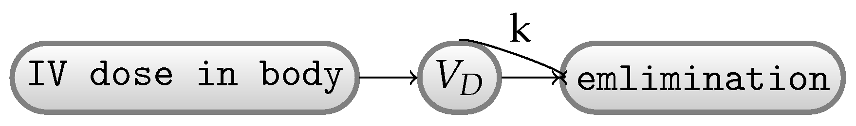
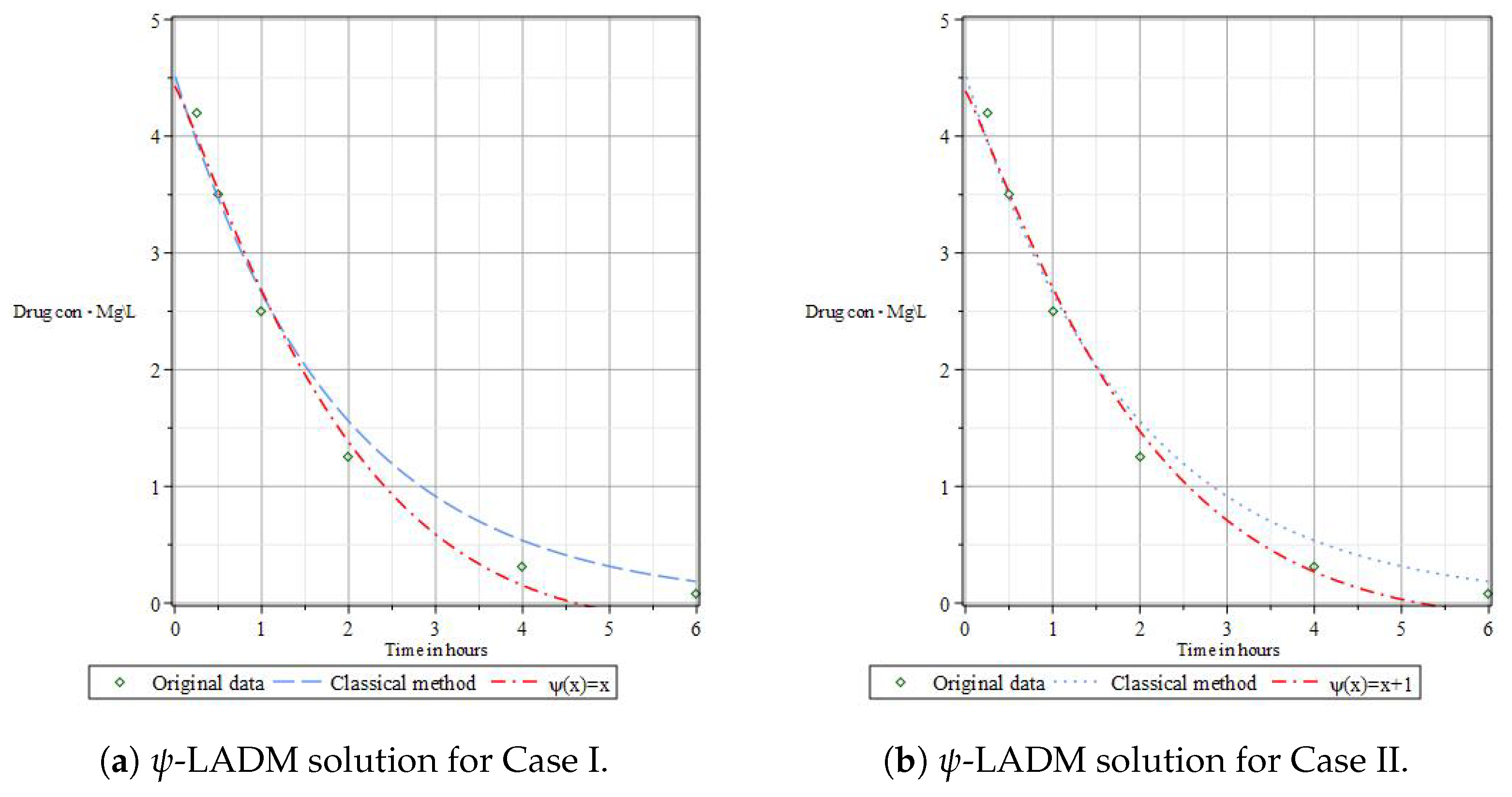
• Case I: Consider the pharmacokinetics IVP for $\psi$-FDE as follows

  $${}^{C}D^{1.13327,x}y\left(x\right)=-0.51749y\left(x\right),y\left(0\right)=20,$$

  (54)

  where $\alpha =1.13327$, $k=0.51749$, and $\psi \left(x\right)=x,$, with the initial dose in body being $y\left(0\right)=20.$
  To solve (54) using $\psi$-LADM, we apply the $\psi$-LT to both sides of the model, with the help of (16), to eventually obtain

  $${\mathcal{L}}_{\psi }\left\{y\left(x\right)\right\}-{\displaystyle \frac{20}{s}}=-{\displaystyle \frac{1}{s^{1.13327}}}{\mathcal{L}}_{\psi }\left\{0.51749y\left(x\right)\right\}.$$

  (55)
  Next, we apply the inverse $\psi$-LT on the latter equation to obtain the following

  $$y\left(x\right)={\mathcal{L}}_{\psi }^{-1}\left\{{\displaystyle \frac{20}{s}}\right\}-{\mathcal{L}}_{\psi }^{-1}\left\{{\displaystyle \frac{1}{s^{1.13327}}}{\mathcal{L}}_{\psi }\left\{0.51749y\left(x\right)\right\}\right\}.$$

  (56)
  Further, the application of the standard ADM process yields

  $$\sum _{n=0}^{\infty }{y}_n\left(x\right)={\mathcal{L}}_{\psi }^{-1}\left\{{\displaystyle \frac{20}{s}}\right\}-{\mathcal{L}}_{\psi }^{-1}\left\{{\displaystyle \frac{1}{s^{1.13327}}}{\mathcal{L}}_{\psi }\left\{0.51749\sum _{n=0}^{\infty }{y}_n\left(x\right)\right\}\right\},$$

  (57)

  that reveals the following recurrent relation

  $$\left\{\begin{array}{c}{y}_0\left(x\right)={\mathcal{L}}_{\psi }^{-1}\left\{{\displaystyle \frac{20}{s}}\right\}=20,\hfill \\ y_n\left(x\right)=-{\mathcal{L}}_{\psi }^{-1}\left\{{\displaystyle \frac{1}{s^{1.13327}}}{\mathcal{L}}_{\psi }\left\{0.51749y_{n-1}\left(x\right)\right\}\right\},n\ge 1.\hfill \end{array}\right.$$

  (58)
  Therefore, some of the $\psi$-LADM terms are recurrently expressed from the above scheme relation as follows

  $$\begin{array}{cc}\hfill y_0\left(x\right)& =20,\hfill \\ \hfill y_1\left(x\right)& =-{\mathcal{L}}_{\psi }^{-1}\left\{{\displaystyle \frac{1}{s^{1.13327}}}{\mathcal{L}}_{\psi }\left\{0.51749\left(20\right)\right\}\right\}=-9.728392289{(\psi \left(x\right)-\psi \left(0\right))}^{1.13327}\hfill \\ & =-9.728392289x^{1.13327},\hfill \\ \hfill y_2\left(x\right)& =-{\mathcal{L}}_{\psi }^{-1}\left\{{\displaystyle \frac{1}{s^{1.13327}}}{\mathcal{L}}_{\psi }\left\{0.51749(-9.728392289x^{1.13327})\right\}\right\}=2.065825777{(\psi \left(x\right)-\psi \left(0\right))}^{2.26654}\hfill \\ & =2.065825777x^{2.26654},\hfill \\ \hfill ⋮\end{array}$$

  which, when summed up, reach the following exact solution (54) as

  $$\begin{array}{cc}\hfill y\left(x\right)& =20-9.728392289x^{1.13327}+2.065825777x^{2.26654}+\cdots ,\hfill \\ \hfill y\left(x\right)& =y_0{E}_{\alpha }\left[(-k)\left({(\psi \left(x\right)-\psi \left(0\right))}^{\alpha }\right)\right]=20E_{1.13327}\left[(-0.51749)\left({\left(x\right)}^{1.13327}\right)\right],\hfill \end{array}$$

  where $E_{(.)}$ is the one-parameter Mittag-Leffler function; see Figure 6a for the graphical illustration of the obtained exact solution, in comparison to the physical dataset from [25].

• Case II: Consider the pharmacokinetics IVP for $\psi$-FDE as follows

  $${}^{C}D^{1.11080,x+1}y\left(x\right)=-0.49621y\left(x\right),y\left(0\right)=20,$$

  (59)

  where $\alpha =1.11080$, $k=0.49621$, and $\psi \left(x\right)=x+1,$, with the initial dose in body being $y\left(0\right)=20.$
  To solve (59) using $\psi$-LADM, $\psi$-LT is applied on both sides of the above model, with the help of (16), to eventually obtain

  $${\mathcal{L}}_{\psi }\left\{y\left(x\right)\right\}-{\displaystyle \frac{20}{s}}=-{\displaystyle \frac{1}{s^{1.11080}}}{\mathcal{L}}_{\psi }\left\{0.49621y\left(x\right)\right\}.$$

  (60)
  Now, upon applying the inverse $\psi$-LT on both sides of the above equation, one obtains

  $$y\left(x\right)={\mathcal{L}}_{\psi }^{-1}\left\{{\displaystyle \frac{20}{s}}\right\}-{\mathcal{L}}_{\psi }^{-1}\left\{{\displaystyle \frac{1}{s^{1.11080}}}{\mathcal{L}}_{\psi }\left\{0.49621y\left(x\right)\right\}\right\}.$$

  (61)
  Next, the application of the ADM procedure gives

  $$\sum _{n=0}^{\infty }{y}_n\left(x\right)={\mathcal{L}}_{\psi }^{-1}\left\{{\displaystyle \frac{20}{s}}\right\}-{\mathcal{L}}_{\psi }^{-1}\left\{{\displaystyle \frac{1}{s^{1.11080}}}{\mathcal{L}}_{\psi }\left\{0.49621\sum _{n=0}^{\infty }{y}_n\left(x\right)\right\}\right\},$$

  (62)

  that leads to the acquisition of the following recursive scheme

  $$\left\{\begin{array}{c}{y}_0\left(x\right)={\mathcal{L}}_{\psi }^{-1}\left\{{\displaystyle \frac{20}{s}}\right\}=20,\hfill \\ y_n\left(x\right)=-{\mathcal{L}}_{\psi }^{-1}\left\{{\displaystyle \frac{1}{s^{1.11080}}}{\mathcal{L}}_{\psi }\left\{0.49621y_{n-1}\left(x\right)\right\}\right\},n\ge 1.\hfill \end{array}\right.$$

  (63)
  Accordingly, some $\psi$-LADM terms for the governing fractional IVP are expressed from the above scheme as follows

  $$\begin{array}{cc}\hfill y_0\left(x\right)& =20,\hfill \\ \hfill y_1\left(x\right)& =-{\mathcal{L}}_{\psi }^{-1}\left\{{\displaystyle \frac{1}{s^{1.11080}}}{\mathcal{L}}_{\psi }\left\{0.49621\left(20\right)\right\}\right\}=-9.433446716{(\psi \left(x\right)-\psi \left(0\right))}^{1.11080}\hfill \\ & =-9.433446716x^{1.11080}\hfill \\ \hfill y_2\left(x\right)& =-{\mathcal{L}}_{\psi }^{-1}\left\{{\displaystyle \frac{1}{s^{1.11080}}}{\mathcal{L}}_{\psi }\left\{0.49621(-9.433446716x^{1.11080})\right\}\right\}=1.988051839{(\psi \left(x\right)-\psi \left(0\right))}^{2.2216}\hfill \\ & =1.988051839x^{2.2216},\hfill \\ \hfill ⋮\end{array}$$

  the net sum of which yields

  $$\begin{array}{cc}\hfill y\left(x\right)& =20-9.433446716x^{1.11080}+1.988051839x^{2.2216}+\cdots .\hfill \\ \hfill y\left(x\right)& =y_0{E}_{\alpha }\left[(-k)\left({(\psi \left(x\right)-\psi \left(0\right))}^{\alpha }\right)\right]=20E_{1.11080}\left[(-0.49621)\left({\left(x\right)}^{1.11080}\right)\right],\hfill \end{array}$$

  where $E_{(.)}$ is the one-parameter Mittag-Leffler function; see Figure 6b for the graphical illustration of the obtained exact solution, in comparison to the physical dataset from [25].

5. Conclusions

FDEs are highly effective tools for modeling diverse real-world physical phenomena, where achieving high-precision solutions is often crucial. The use of $\psi$-Caputo fractional derivatives provides added flexibility in these models, uncovering hidden characteristics within complex real-life phenomena. This study introduced $\psi$-LADM for the class of $\psi$-Caputo differential equations and further applied the resulting scheme to some test IVPs for fractional differential equations. Furthermore, this study extended the method’s application to real-world physical models, particularly in analyzing pharmacokinetics. The solutions obtained aligned closely with available exact solutions for the test problems, while the pharmacokinetics model results demonstrated an excellent fit with existing data. Overall, this approach proves to be reliable and applicable to a range of $\psi$-FDEs with various initial and boundary conditions.

References

1. He, J.H. Fractal calculus and its geometrical explanation. Results Phys. 2018, 10, 272–276. [Google Scholar] [CrossRef]
2. Wang, Q.; Shi, X.; He, J.H.; Li, Z.B. Fractal calculus and its application to explanation of biomechanism of polar bear hairs. Fractals 2018, 26, 1850086. [Google Scholar] [CrossRef]
3. Kilbas, A.A.; Srivastava, H.M.; Trujillo, J.J. Theory and Applications of Fractional Differential Equations; Elsevier: Amsterdam, The Netherlands, 2006; Volume 204. [Google Scholar]
4. Teodoro, G.S.; Machado, J.T.; De Oliveira, E.C. A review of definitions of fractional derivatives and other operators. J. Comput. Phys. 2019, 388, 195–208. [Google Scholar] [CrossRef]
5. Milici, C.; Draganescu, G.; Machado, J.T. Introduction to Fractional Differential Equations; Springer: Berlin/Heidelberg, Germany, 2018; Volume 25. [Google Scholar]
6. Almeida, R. A Caputo fractional derivative of a function with respect to another function. Commun. Nonlinear Sci. Numer. Simul. 2017, 44, 460–481. [Google Scholar] [CrossRef]
7. Almeida, R.; Malinowska, A.B.; Monteiro, M.T.T. Fractional differential equations with a Caputo derivative with respect to a kernel function and their applications. Math. Methods Appl. Sci. 2018, 41, 336–352. [Google Scholar] [CrossRef]
8. Derbazi, C.; Baitichezidane, Z.; Benchohra, M. Coupled system of ψ-Caputo fractional differential equations without and with delay in generalized Banach spaces. Results Nonlinear Anal. 2022, 5, 42–61. [Google Scholar] [CrossRef]
9. Boutiara, A.; Abdo, M.S.; Benbachir, M. Existence results for ψ-Caputo fractional neutral functional integro-differential equations with finite delay. Turk. J. Math. 2020, 44, 2380–2401. [Google Scholar] [CrossRef]
10. Khan, H.N.A.; Zada, A.; Khan, I. Analysis of a Coupled System of ψ-Caputo Fractional Derivatives with Multipoint–Multistrip Integral Type Boundary Conditions. Qual. Theory Dyn. Syst. 2024, 23, 129. [Google Scholar] [CrossRef]
11. Aydi, H.; Jleli, M.; Samet, B. On positive solutions for a fractional thermostat model with a convex-concave source term via ψ-Caputo fractional derivative. Mediterr. J. Math. 2020, 17, 16. [Google Scholar] [CrossRef]
12. Alharbi, F.M.; Zidan, A.M.; Naeem, M.; Shah, R.; Nonlaopon, K. Numerical investigation of fractional-order differential equations via ψ-Haar wavelet method. J. Funct. Spaces 2021, 2021, 3084110. [Google Scholar] [CrossRef]
13. Almeida, R.; Jleli, M.; Samet, B. A numerical study of fractional relaxation-oscillation equations involving ψ-Caputo fractional derivative. Rev. Real Acad. Cienc. Exactas Fís. Nat. Ser. A Mat. 2019, 113, 1873–1891. [Google Scholar] [CrossRef]
14. Jarad, F.; Abdeljawad, T. Generalized fractional derivatives and Laplace transform. Discret. Contin. Dyn. Syst.-Ser. S 2020, 13, 709–722. [Google Scholar] [CrossRef]
15. Fahad, H.M.; Rehman, M.U.; Fernandez, A. On Laplace transforms with respect to functions and their applications to fractional differential equations. Math. Methods Appl. Sci. 2023, 46, 8304–8323. [Google Scholar] [CrossRef]
16. Alsulami, M.; Alyami, M.; Al-Mazmumy, M.; Alsulami, A. Semi-analytical investigation for the ψ-Caputo fractional relaxation-oscillation equation using the decomposition method. Eur. J. Pure Appl. Math. 2024, 17, 2311–2398. [Google Scholar]
17. Alsulami, A.S.; Al-Mazmumy, M.; Alyami, M.A.; Alsulami, M. Application of Adomian decomposition method to a generalized fractional Riccati differential equation (ψ-FRDE). Adv. Differ. Equ. Control Process. 2024, 31, 531–561. [Google Scholar]
18. Al-Mazmumy, M.; Alyami, M.A.; Alsulami, M.; Alsulami, A.S. Efficient modified Adomian decomposition method for solving nonlinear fractional differential equations. Int. J. Anal. Appl. 2024, 22, 76. [Google Scholar] [CrossRef]
19. Dhandapani, P.B.; Leiva, V.; Martin-Barreiro, C.; Rangasamy, M. On a novel dynamics of a SIVR model using a Laplace Adomian decomposition based on a vaccination strategy. Fractal Fract. 2023, 7, 407. [Google Scholar] [CrossRef]
20. Yunus, A.O.; Olayiwola, M.O.; Adedokun, K.A.; Adedeji, J.A.; Alaje, I.A. Mathematical analysis of fractional-order Caputo’s derivative of coronavirus disease model via Laplace Adomian decomposition method. Beni-Suef Univ. J. Basic Appl. Sci. 2022, 11, 144. [Google Scholar] [CrossRef]
21. Alsulami, M.; Alyami, M.; Al-Mazmumy, M.; Alsulami, A. Reliable computational method for systems of fractional differential equations endowed with ψ-Caputo fractional derivative. Contemp. Math. 2024, in press. [Google Scholar]
22. Awadalla, M.; Noupoue, Y.Y.Y.; Asbeh, K.A.; Ghiloufi, N. Modeling drug concentration level in blood using fractional differential equation based on ψ-Caputo derivative. J. Math. 2022, 2022, 9006361. [Google Scholar] [CrossRef]
23. Almeida, R. What is the best fractional derivative to fit data? Appl. Anal. Discret. Math. 2017, 11, 358–368. [Google Scholar] [CrossRef]
24. Awadalla, M.; Yameni Noupoue, Y.Y.; Asbeh, K.A. ψ-Caputo logistic population growth model. J. Math. 2021, 2021, 8634280. [Google Scholar] [CrossRef]
25. Ahmed, T.A. Pharmacokinetics of Drugs Following IV Bolus, IV Infusion, and Oral Administration. Basic Pharmacokinetic Concepts and Some Clinical Applications; IntechOpen: Rijeka, Croatia, 2015; Volume 10. [Google Scholar]
Figure 1. ψ -LADM solutions with respect to different kernels for (31).
Mathematics 12 03499 g001
Figure 2. ψ -LADM solutions with respect to the different kernels and α for (36).
Mathematics 12 03499 g002
Figure 3. ψ -LADM solutions with respect to the different kernels for (42).
Mathematics 12 03499 g003
Figure 4. ψ -LADM solutions for various ψ functions and various α of (47).
Mathematics 12 03499 g004
Figure 5. One-compartment open model: intravenous bolus administration.
Mathematics 12 03499 g005
Figure 6. ψ -LADM solutions for the fractional pharmacokinetics IVP in (54) and (59).
Mathematics 12 03499 g006