A Novel Exploration of Diffusion Process Based on Multi-Type Galton–Watson Forests

Abstract

Diffusion is a commonly used technique for spreading information from point to point on a graph. The rationale behind diffusion is not clear. The multi-type Galton–Watson forest is a random model of population growth without space or any other resource constraints. In this paper, we use the degenerated multi-type Galton–Watson forest (MGWF) to interpret the diffusion process, corresponding vertices to types and establishing an equivalence relationship between them. With the two-phase setting of the MGWF, one can interpret the diffusion process and the Google PageRank system explicitly. It also improves the convergence behavior of the iterative diffusion process and Google PageRank system. We validate the proposal by experiment while providing new research directions.

1. Introduction

The diffusion process is a phenomenon in which particles spontaneously diffuse from a region of high concentration to a region of low concentration so that the system tends to a stable state. Because of its ability to capture the intrinsic manifold structure of data, diffusion processes are widely used in many areas of machine learning, such as information retrieval [1,2,3,4,5]; clustering [6,7]; significance detection [8,9]; image segmentation [4,10]; and semi-supervised learning [5,11].

Technically, the undirected graph $\mathcal{G}=(V,E)$ consists of N nodes $v_i\in V,$ and edges $e_{ij}\in E$. The edges $e_{ij}$ can be weighted by their affinity value $A_{ij}$. The diffusion process can be interpreted as a Markov random walk on the graph $\mathcal{G}$, where the initial distribution $F_0$ containing the initial information, for example, in affinity learning, the initial distribution is the initially constructed affinity matrix. Information is transferred according to the transfer matrix P, and the iteration criterion is

$$\begin{array}{c}\hfill F_n=F_{n-1}P,\end{array}$$

(1)

where $P=D^{-1}A$, A is the affinity matrix of $\mathcal{G}$, $D_{ii}={\Sigma }_{k=1}^N{A}_{ik}$ is the diagonal matrix.

To address the interpretation dilemmas of diffusion process, this paper employs the MGWF with a degenerate branching law model to map graph points to distinct types, providing a multi-faceted explanation of the diffusion process. Specifically, we innovatively introduce the concept of particle mutation, divide each step of the diffusion process into two phases. It can understand the diffusion process more clearly, and inspire us to learn the diffusion process in a general setting. Furthermore, the model of MGWF with mutation and immigration can be used to explain the well-known Google PageRank system. This will also inspire us to interpret the Google PageRank system from a new perspective.

In summary, the main contributions of this article are as follows:

•

It introduces the novel concept of mutation into the MGWF with the degenerated branching law, where each step of the diffusion process is divided into two phases—the branching phase and the mutation phase. Such an explanation provides novel insight on the rationale of the diffusion process from a longitudinal perspective. Moreover, it is beneficial for the more general diffusion process.

•

It proves the sequence convergence of affinity matrix generated by the diffusion process under the given assumption. To our best knowledge, this is the first time that the convergence of the diffusion process has been proved theoretically.

•

It interprets the Google PageRank system well by extending the MGWF by introducing immigration.

•

It proposes a variant of the diffusion process in which the mutation probability can change in the framework of branching and mutation. It is a more general diffusion process that includes the original as a special case.

The remainder of this paper is as follows. Section 2 introduces the MGWF model in detail. In Section 3 and Section 4, we explain the diffusion process and the Google PageRank system under the new model, respectively. Section 5 shows the experimental results with the probability matrix change. Section 6 concludes this article.

2. Preliminaries

The branching process is also known as Galton–Watson process (GW process) which is also a Markov chain. It can deal with a mathematical representation for the population changes in which their members can reproduce and die, subject to laws of chance.

Definition 1

(Branching process). Let ξ be non-negative integer random variables, where the distribution is $p_k=P(\xi =k),k\ge 0,P_0<1$. Suppose that the number of offspring produced by a species follows the distribution of ξ, and the reproduction of each individual within the species is independent. The number of individuals in the first generation is $Z_1$, and naturally there is

$$\begin{array}{c}\hfill Z_{n+1}=\sum _{i=1}^{Z_n}{\xi }_{n+1,i},\end{array}$$

(2)

where ${\xi }_{n+1,i}$ can be thought of as the number of members in the $(n+1)$-th generation which are the offspring of the i-th member of the n generation.

There is a list of random variables $\left\{Z_n\right\}$ which take non-negative integer values. $Z_n$ satisfies the recursive relation. Then, such a random process $\left\{Z_n\right\}$ is a Markov chain with state space $\mathbb{Z}$ and transition probability

$$\begin{array}{c}\hfill P_{ij}=P(\sum _{k=1}^i{\xi }_k=j).\end{array}$$

(3)

The particles may be of different types depending on their age, energy, position, or other factors. However, the type of all particles is the same in the GW process. Following, it introduces the multi-type GW process.

Definition 2

(N-type GW process). Given the initiated state as

$$\begin{array}{c}\hfill {\mathbf{Z}}_1=(Z_{1,1},\dots ,Z_{1,N})\end{array}$$

(4)

where $Z_{1,k}\in {\mathbb{Z}}_{+},k=1,\dots N$, is the number of individuals of k-type. For the nth generation,

$$\begin{array}{c}\hfill {\mathbf{Z}}_n=(Z_{n,1},Z_{n,2}\dots ,Z_{n,N})\end{array}$$

(5)

where $Z_{n,j}$ represents the number of particles of j-type in the $nth$ generation. Then, ${\left\{{\mathbf{Z}}_n\right\}}_{n\ge 0}$ is a N-type GW process.

It assumes that the parent i lives for a unit of time and, upon death, produces children of all types and according to the offspring distribution $P^i\left(j\right)$ and the independence of other individuals. The case is vividly called a multi-type Galton–Watson forest (MGWF) [12,13,14,15,16].

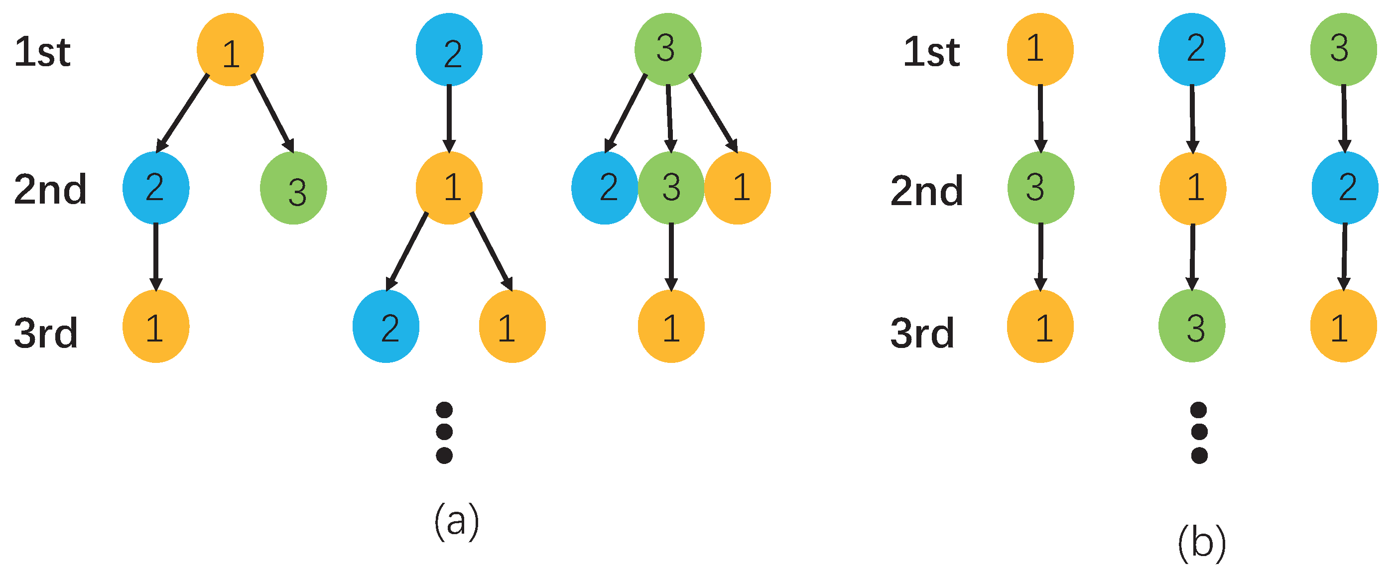
Next, a special N-type GWF is introduced. The initiated state

$$\begin{array}{c}\hfill {\mathbf{Z}}_0={\mathbf{e}}_i\end{array}$$

(6)

where ${\mathbf{e}}_i,i=1,2,\dots ,N$ denotes the i-th component as 1, and the remaining is zero. The ancestor lives for a unit of time and produces one child of all types upon death according to the offspring distribution $\left\{P^{{\mathbf{e}}_i}\left({\mathbf{e}}_j\right)\right\}=\left\{P^i\left(j\right)\right\}$, where

$$\begin{array}{c}\hfill {\mathbf{P}}^i\left(\{\mathbf{Z}\in {\mathbb{N}}^N:{\Sigma }_{j=1}^N{Z}_j\ne 1\right\})=0\end{array}$$

(7)

i.e., each parent produces only one offspring. In this way, the number of multi-type branching tree formed in the forest is N. From [12,13], it names the MGWF with the degenerate branching law. It is called MGWF in this paper. The difference between the MGWF and the MGWF with the degenerated branching law is graphically illustrated in Figure 1.

Example 1.

There are three types of particles in MGWF, i.e., $N=3$. The 3-type GW forest with the degenerated branching law P is shown in Figure 1b. The branching law matrix is

$$\begin{array}{c}\hfill P_{3\times 3}=\left(\begin{array}{ccc}0& {\displaystyle \frac{2}{3}}& {\displaystyle \frac{1}{3}}\\ {\displaystyle \frac{2}{5}}& 0& {\displaystyle \frac{3}{5}}\\ {\displaystyle \frac{1}{5}}& {\displaystyle \frac{4}{5}}& 0\end{array}\right).\end{array}$$

3. Mutations in the MGWF

3.1. The Mutations

Let us consider mutation in the framework of MGWF with the degenerated branching law [17,18]. In this paper, we propose a novel variant of mutation which can better conform to the actual situation, and more importantly, it provides the new insight into the rationale of the diffusion process by separating it into two phases, branching and mutation.

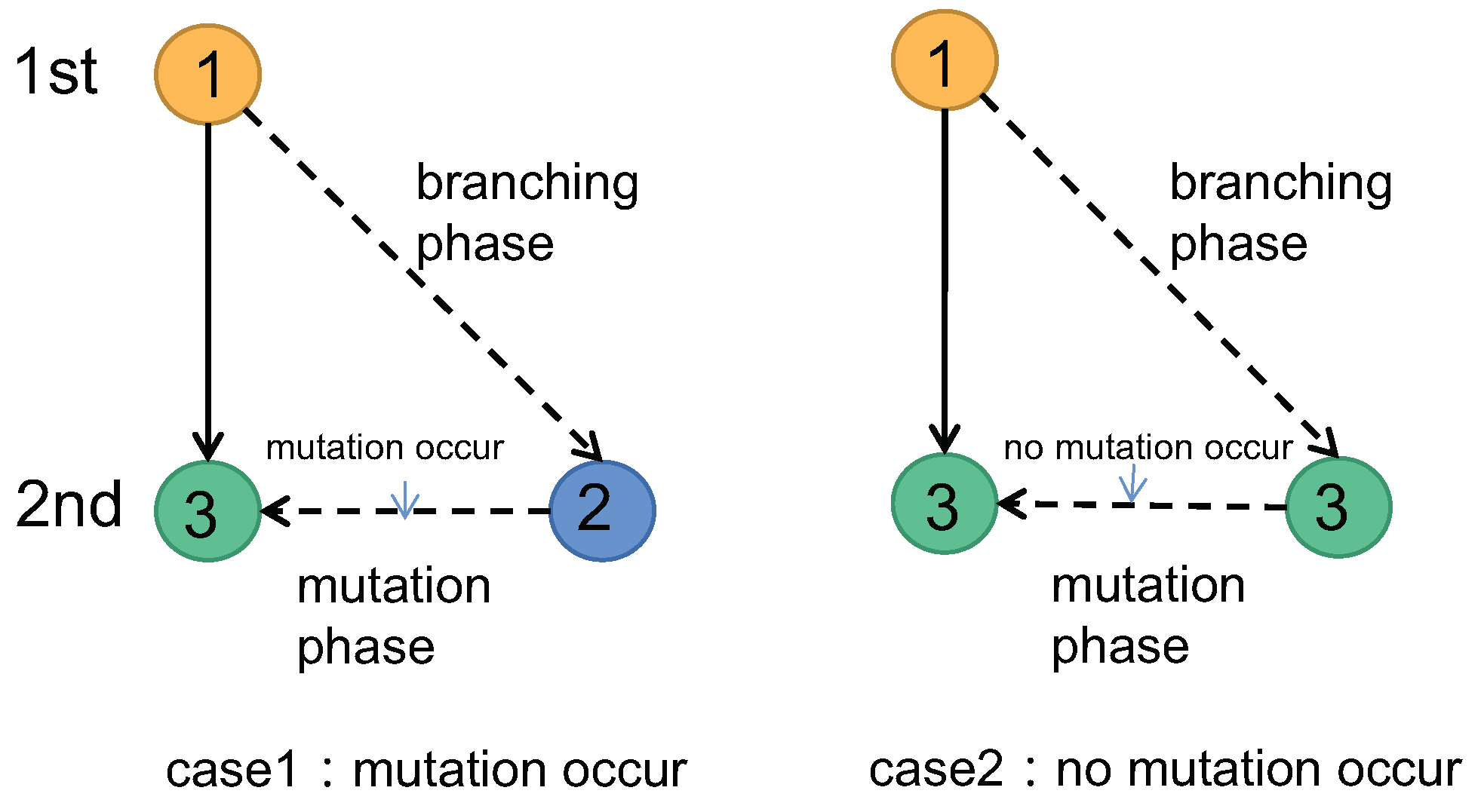
Definition 3

(Mutation). When the mutation time is ignored, a unit of time is divided into two phases, the branching phase and the mutation phase.

(i) 

In the branching phase. An i-type particle produces a j-type particle according to the branching law $P^i\left(j\right)$.

(ii) 

In the mutation phase.

The mutation occurs: the j-type particle may mutate into a k-type particle according to the probability of mutation $T^j\left(k\right),j\ne k,i,j,k=1,2,\dots ,N$.

No mutation occurs: the j-type particle may also remain unchanged in type with probability $T^j\left(j\right)$.

The two cases in the mutation phase are shown in Figure 2.

Naturally, when mutations are considered, the branching law matrix is change, and the iterative process is as follows.

Let $P_1^i\left(j\right)=P^i\left(j\right)$, and T is a probability matrix of mutation. At time 0, there is an i-type ancestor; after a unit of time, it has a j-type offspring. Then, in the second generation,

$$\begin{array}{c}\hfill P_2^i\left(j\right)=P_1^i\left(j\right)T^j\left(j\right)+{\Sigma }_{k\ne j}{P}_1^i\left(k\right)T^k\left(j\right).\end{array}$$

(8)

Its matrix form is,

$$\begin{array}{c}\hfill P_2=P_{1}T.\end{array}$$

(9)

Iteratively, for the $nth$ generation,

$$\begin{array}{c}\hfill P_n=P_{n-1}T=P{T}^{n-1},\end{array}$$

(10)

where $P_n=P{T}^{n-1}$ is the expansion of the entire iterative process. $P_n=P_{n-1}T$ focuses on one generation, while $P_n=P{T}^{n-1}$ focuses on the entire process. Next, we use one example to show the iteration process.

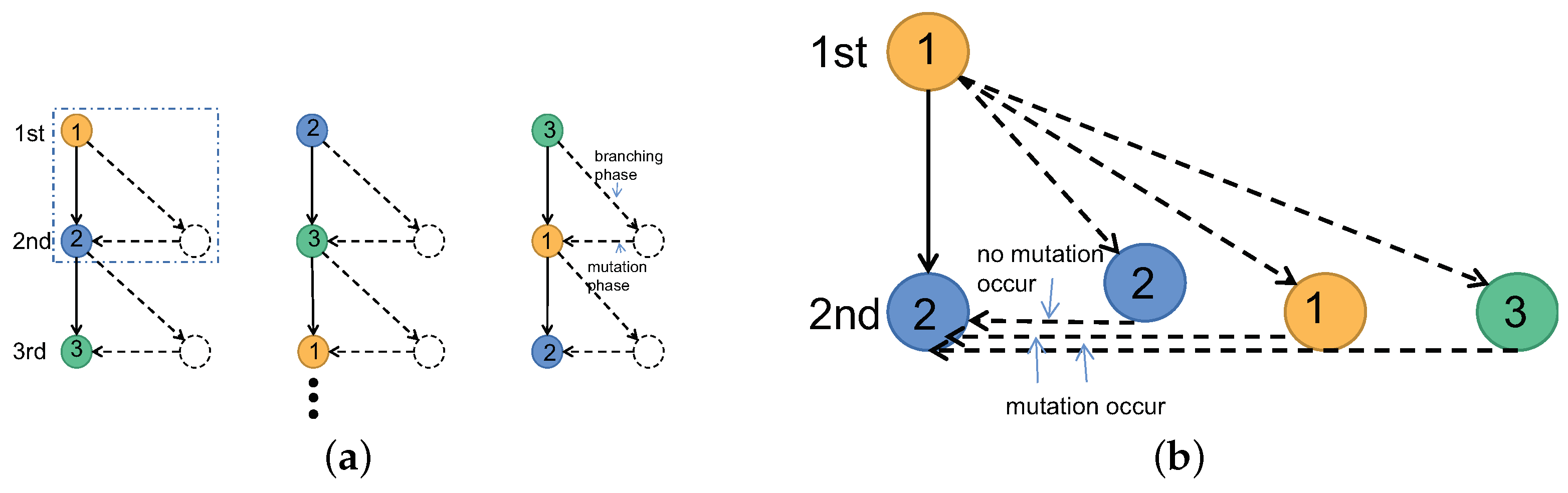
Example 2

(The continuation of Example 1). Let the probability matrix of mutation $T=P$. The 3-type GW forest with mutation and the mutation details are shown in Figure 3.

It shows the branching low matrix of the second generation and third generation

$$\begin{array}{c}\hfill P_2=PT=\left(\begin{array}{ccc}{\displaystyle \frac{1}{3}}& {\displaystyle \frac{4}{15}}& {\displaystyle \frac{2}{5}}\\ {\displaystyle \frac{3}{25}}& {\displaystyle \frac{56}{75}}& {\displaystyle \frac{2}{15}}\\ {\displaystyle \frac{8}{25}}& {\displaystyle \frac{2}{15}}& {\displaystyle \frac{41}{75}}\end{array}\right)\end{array}$$

and

$$\begin{array}{c}\hfill P_3=P_{2}T=P{T}^2=\left(\begin{array}{ccc}{\displaystyle \frac{14}{75}}& {\displaystyle \frac{122}{225}}& {\displaystyle \frac{61}{225}}\\ {\displaystyle \frac{122}{375}}& {\displaystyle \frac{14}{75}}& {\displaystyle \frac{61}{125}}\\ {\displaystyle \frac{61}{375}}& {\displaystyle \frac{244}{375}}& {\displaystyle \frac{14}{75}}\end{array}\right).\end{array}$$

Next, we discuss the convergence of the above iterative process.

3.2. The Stable State

It introduces a few concepts and lemmas that come from the literature [19,20].

Definition 4

(communicate [19]). Let $i,j\in \mathbb{S}$ be two states of a Markov chain with transition matrix T. Then, state i communicates with state j if there exist non-negative integers m and n such that $T_{j,i}^m>0$ and $T_{i,j}^n>0$.

Definition 5

(irreducible [20]). A Markov chain with finite-state space $\mathbb{S}$ and transition matrix T is said to be irreducible if for all $i,j\in \mathbb{S}$ are communicated.

Definition 6

(aperiodic [19]). The period $d\left(i\right)$ of a state i of a Markov chain is the greatest common divisor of all time steps n for which $T_{ii}^n>0$. If the period is 1, the state is aperiodic.

If a Markov chain is irreducible, the period of the chain is the period of its single communication class. If the period of every communication class is $d=1$, then the Markov chain is aperiodic.

Definition 7

(regular [19]). A stochastic matrix T is regular if some power $T^k$ contains only strictly positive entries.

Lemma 1.

Let T be the transition matrix for an irreducible, aperiodic Markov chain. Then, T is a regular matrix.

Proof. 

For detailed proof, see page C-39 of the literature [19]. □

Lemma 2

(Ref. [19]). If T is a regular $m\times m$ transition matrix of Markov chain with $m\ge 2$, then the following statements are all true.

(1) 

There is a stochastic matrix Π such that ${lim}_{n\to \infty }{T}^n=\Pi$.

(2) 

Each row of Π is the same probability vector π.

(3) 

For any initial probability vector ${\mathbf{x}}_{\mathbf{0}},{lim}_{n\to \infty }{\mathbf{x}}_{\mathbf{0}}{T}^n=\mathit{\pi }$.

(4) 

The vector π is the unique probability vector that is an eigenvector of T associated with the eigenvalue 1, i.e., $\mathit{\pi }=\mathit{\pi }T$.

Proof. 

For detailed proof, see the Appendix (page C-65) of reference [19]. □

As described above, to prove the convergence of the iterative process, we make the following statement.

Assumption 1.

The MGWF with mutation is a finite-state Markov chain.

Assumption 2.

The MGWF with mutation is an irreducible chain.

Assumption 3.

The MGWF with mutation is required to be an aperiodic chain.

Theorem 1.

Suppose Assumptions 1–3 hold. Then, the MGWF with mutation has a unique stationary distribution Π, s.t.

$$\begin{array}{c}\hfill \underset{n\to \infty }{lim}{T}^n=\Pi \end{array}$$

(11)

where each row of Π is the same probability vector π which is the unique probability vector that is an eigenvector of T associated with the eigenvalue 1.

Proof. 

On the one hand, we prove that the limit exists. Since Assumptions 1–3 are satisfied, according to Lemma 1, the probability matrix of mutation T is regular. From Lemma 2 (1), $\underset{n\to \infty }{lim}{T}^n=\Pi$.

On the other hand, we analyze the composition of the limit matrix $\Pi$. From Lemma 2, (2) and (4), the limit matrix $\Pi ={\mathit{\pi }}^{\top }\mathbf{1}$, where $\mathit{\pi }$ is an eigenvector of T associated with the eigenvalue 1.

In summary, the conclusion of Theorem 1 is proved. □

When the MGWF with mutations reaches a stable state $\Pi$, the branching law is no longer affected by the mutation.

Example 3

(The continuation of Example 2). Let the probability matrix of mutation $T=P$, where the transition matrix P is given in Example 1. It is verified that $k=2,T_{ij}^2>0$ for all $i,j\in \{1,2,\dots ,N\}$, so T is regular, satisfying the Lemma 2 condition. It sets the threshold to $1\times {10}^{-8}$,

$$\begin{array}{c}\hfill P^{88}=\left(\begin{array}{ccc}{\displaystyle \frac{39}{164}}& {\displaystyle \frac{35}{82}}& {\displaystyle \frac{55}{164}}\\ {\displaystyle \frac{39}{164}}& {\displaystyle \frac{35}{82}}& {\displaystyle \frac{55}{164}}\\ {\displaystyle \frac{39}{164}}& {\displaystyle \frac{35}{82}}& {\displaystyle \frac{55}{164}}\end{array}\right)\end{array}$$

and iterating $P^{89},P^{90},\dots$ again, it no longer changes, i.e., the particle mutation will not affect the branching law of the MGWF.

3.3. Interpretation of Diffusion Process

In general, the diffusion process starts from a $N\times N$ affinity matrix A. It interprets the matrix A as a graph $\mathcal{G}=(V,E)$, consisting of N nodes $v_i\in V$, and edges $e_{ij}\in E$ that link nodes to each other, fixing the edge weights to provide affinity values with $A_{ij}$. The diffusion processes spread the affinity values through the entire graph, based on the transition matrix. When using a random walk on a graph to explain the diffusion process, there are three steps: (1) initialization; (2) definition of the transition matrix; and (3) definition of the diffusion process.

In this paper, we use the model of MGWF with mutation to explain the diffusion process from a new perspective. It regards the N vertices of the graph corresponding to the N different particle types, and the transition of the random walk between nodes corresponds to the iteration of the parent which produces offspring in MGWF with the mutation. And the unit of time for each iteration is divided into two phases, the branching phase and the mutation phase.

Assume that the initial branching law and the probability matrix of mutation are given. To ensure that the initial branching law is a row-stochastic matrix, it takes $F_0=P=D^{-1}A$, where $D=diag\left(D_{ii}\right),D_{ii}={\Sigma }_{j=1}^N{A}_{ij}$, and especially the probability matrix of mutation $T=P=D^{-1}A$. After the first unit time, the branching law of the first generation is given by

$$\begin{array}{c}\hfill F_1=F_{0}T.\end{array}$$

(12)

Eventually, the branching law of the $nth$ generation is

$$\begin{array}{c}\hfill F_n=F_{n-1}T=F_0{T}^n.\end{array}$$

(13)

Assuming Assumptions 1–3 hold, from Theorem 1, the branching law reaches a stable state, that is, the branching law will no longer be affected by the mutation.

The correspondence between the diffusion process and the MGWF with the mutation is shown in

Table 1. The correspondence between diffusion process and MGWF with mutation.

Diffusion Process	MGWF with Mutation
N nodes in the graph	N types of particle
Edges in the graph	Particle type change
An iteration of the diffusion process	A unit time of MGWF
Initialization $F_0=P$	Initial branching law matrix $F_0=P$
Transition matrix P	The probability matrix of mutation $T=P$
Update scheme $F_n=F_{n-1}P$	Update scheme $F_n=F_{n-1}T$

.

In this section, we establish the relationship between the diffusion process and the MGWF with mutation. We prove the sequence convergence of the diffusion process under the given assumption. To our best knowledge, this is the first time that the convergence of the diffusion process has been proved theoretically. Next, we propose the immigration concept for the MGWF and discuss its relationship with the Google Pagerank system.

4. The MGWF with Immigration and the Google PageRank System

4.1. The MGWF with Mutation and Immigration

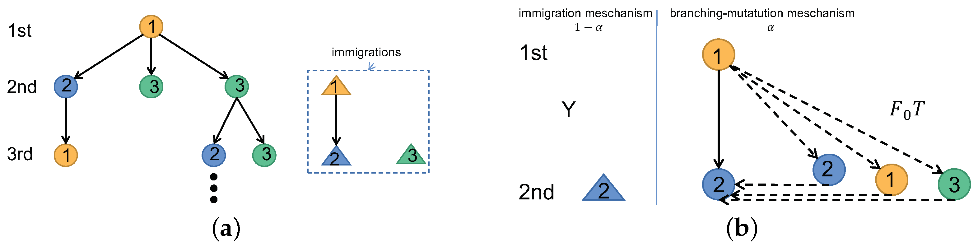
The classic MGWF has a wide range of extensions, and one of the important extensions is the GW process with immigration [21,22,23,24]. In this study, state-independent immigration is considered. The classical theory of immigration is to introduce immigrants to ensure that the entire forest does not become extinct so that immigrant particles can enter the forest and produce offspring together with the original particles as shown in Figure 4a.

In an N-type GWF with the mutations system, for every tree and every generation, there may be an immigrant of the j-type particle entering with probability $b_j,j=1,2,\dots ,N$ and ${\Sigma }_{j=1}^N{b}_j=1$. When it is observed that an i-type particle in the first generation has a child of the j type in the second generation, there are two possible mechanisms:

(1)

Generated by a branching–mutation mechanism with probability $\alpha ,\alpha \in (0,1)$, i.e., an i-type particle produces a j-type particle in the branching–mutations mechanism.

(2)

Acted by the immigration mechanism with probability $(1-\alpha )$, i.e., in the second generation, an immigrant particle of the j type enters directly, the branching–mutations mechanism no longer works.

Therefore, the branching law in the second generation,

$$\begin{array}{c}\hfill P_2^i\left(j\right)=\alpha \left(P_1^i\left(j\right)T^j\left(j\right)+{\Sigma }_{k\ne j}{P}_1^i\left(k\right)T^k\left(j\right)\right)+(1-\alpha )b_j,i,j,k=1,2,\dots ,N.\end{array}$$

(14)

The matrix form is

$$\begin{array}{c}\hfill P_2=\alpha P_{1}T+(1-\alpha )Y\end{array}$$

(15)

where

$$\begin{array}{c}\hfill Y=\left(\begin{array}{cccc}{b}_1& b_2& \cdots & b_N\\ b_1& b_2& \cdots & b_N\\ ⋮& ⋮& ⋮& ⋮\\ b_1& b_2& \cdots & b_N\end{array}\right).\end{array}$$

(16)

Figure 4b shows the relationship between the immigration mechanism and the branching–mutation mechanism.

Set

$$\begin{array}{c}\hfill F_0=P,T=P,\end{array}$$

(17)

and the convergence of this process is given below.

Theorem 2.

Suppose Assumptions 1–3 hold. Then, the set $\left\{F_n\right\}$ generated from the MGWF with the mutation and immigration is the convergence, that is, the limit ${lim}_{n\to \infty }{F}_n$ exists.

Proof. 

$$\begin{array}{c}\hfill F_n=\alpha F_{n-1}T+(1-\alpha )Y={\alpha }^n{P}^{n+1}+(1-\alpha )Y{\Sigma }_{k=0}^{n-1}{\alpha }^k{P}^k\end{array}$$

(18)

Since $T=P$ is regular, which is explained in Section 4.2, which meets the condition of Lemma 2, the limit ${lim}_{n\to \infty }{P}^{n+1}$ exists. And for ${\Sigma }_{k=0}^{n-1}{\alpha }^k{P}^k$, since the eigenvalue of $\alpha P$, $\rho \left(\alpha P\right)<1$, the limit of ${\Sigma }_{k=0}^{n-1}{\left(\alpha P\right)}^k$ exists when $n\to \infty$. Consequently, the ${lim}_{n\to \infty }{F}_n$ exists. □

4.2. The Google PageRank System

One of the most successful diffusion processes is the Google PageRank system. It was originally designed to objectively rank webpages by measuring people’s interest in the relevant webpages. In the Google PageRank system, in addition to walking on neighboring nodes with a probability $\alpha \in (0,1)$, the particle is also considered to jump to an arbitrary node with a very small probability $(1-\alpha )$, following the update mechanism below:

$$\begin{array}{c}\hfill F_{n+1}=\alpha F_{n}P+(1-\alpha )Y\end{array}$$

(19)

$N\times N$ matrix Y is a stacking of row vectors $\mathbf{y}$, and $\mathbf{y}$ defines the probabilities of randomly jumping to the corresponding nodes.

We use the MGWF with mutation and immigration model to explain the extension of the diffusion process. For convenience, we make the following transformation:

$$\begin{array}{c}\hfill F_{n+1}=\alpha F_{n}P+(1-\alpha )Y\end{array}$$

(20)

$$\begin{array}{c}\hfill =\left(\begin{array}{cc}\alpha F_n& (1-\alpha )I\end{array}\right)\left(\begin{array}{c}P\\ Y\end{array}\right)\end{array}$$

(21)

In the above model, the branching law of $n$th generation is $\left(\begin{array}{cc}\alpha F_n& (1-\alpha )I\end{array}\right)$, where the branching–mutation mechanism works with probability $\alpha$ and the branching law matrix is $F_n$. The immigration mechanism works with probability $(1-\alpha )$, and the branching law matrix is I; the probability matrix of mutation is $\left(\begin{array}{c}P\\ Y\end{array}\right)$ in the mutation phase, where $P,Y$ respectively are the mutation probability of MGWF with the mutation mechanism and immigration mechanism.

We can explain the diffusion process and the Google PageRank system in the same framework model through the proposed two-phase setting. The initial branching law matrix is $F_0=\left(\begin{array}{cc}\alpha P& (1-\alpha )I\end{array}\right)$ in the branching phase. And the probability matrix of mutation is $T=\left(\begin{array}{c}P\\ Y\end{array}\right)$ in the mutation phase. The iteration rule is $F_{n+1}=F_{n}T$. When $\alpha =1$, it is the diffusion process $F_{n+1}=F_{n}P$; when $\alpha \in (0,1)$, it is the Google PageRank system $F_{n+1}=\alpha F_{n}P+(1-\alpha )Y$ as shown in

Table 2. The same framework model of diffusion process and Google PageRank system.

The Framework	$\mathit{\alpha }$	The Model
$F_{n+1}=\left(\begin{array}{cc}\alpha F_n& (1-\alpha )I\end{array}\right)\left(\begin{array}{c}P\\ Y\end{array}\right)$	$\alpha =1$	The diffusion process
	$\alpha \in (0,1)$	The Google PageRank system

.

In summary, we propose the two-phase MGWF setting and explain the diffusion process and the Google PageRank system. It is a new perspective to understand the diffusion process. Further, it extends the diffusion process and speeds up the iteration process as shown in the examples below.

5. Simulations

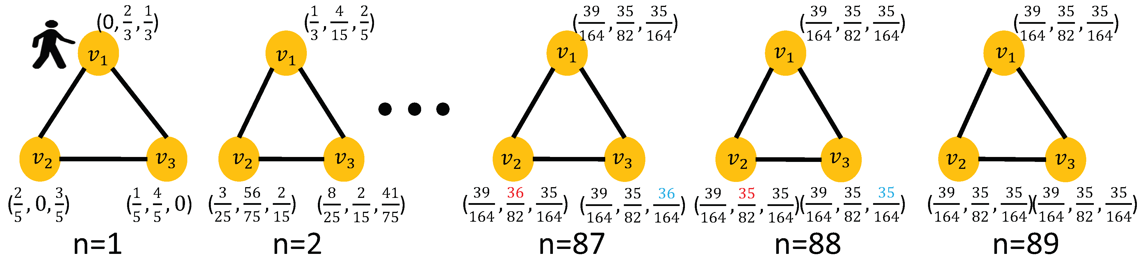
Example 4

(The continuation of Example 3). Let the initial value $F_0=P$, the transition matrix P which is given in Example 1, and the iteration rule $F_{n+1}=F_{n}P$. We explain the diffusion process by random walk and MGWF, respectively.

(i) 

Random walk on graph

For the initial value $F_0=P$, the probability that the particle starts at ${\mathbf{v}}_1,{\mathbf{v}}_2$ and ${\mathbf{v}}_2$ is $\left(\begin{array}{ccc}0& {\displaystyle \frac{2}{3}}& {\displaystyle \frac{1}{3}}\end{array}\right),\left(\begin{array}{ccc}{\displaystyle \frac{2}{5}}& 0& {\displaystyle \frac{3}{5}}\end{array}\right)$ and $\left(\begin{array}{ccc}{\displaystyle \frac{1}{5}}& {\displaystyle \frac{4}{5}}& 0\end{array}\right)$. With the transition matrix P, and the iteration rule $F_{n+1}=F_{n}P$, we use the binary norm of the matrix $\parallel F_n-F_{n-1}{\parallel }_2$ to measure the convergence of $F_n$ with an accuracy of $1\times {10}^{-8}$. We find that the diffusion process can reach this approximate stable state through 88 iterations. The random walk on the graph with three nodes is shown in Figure 5.

(ii)

MGWF

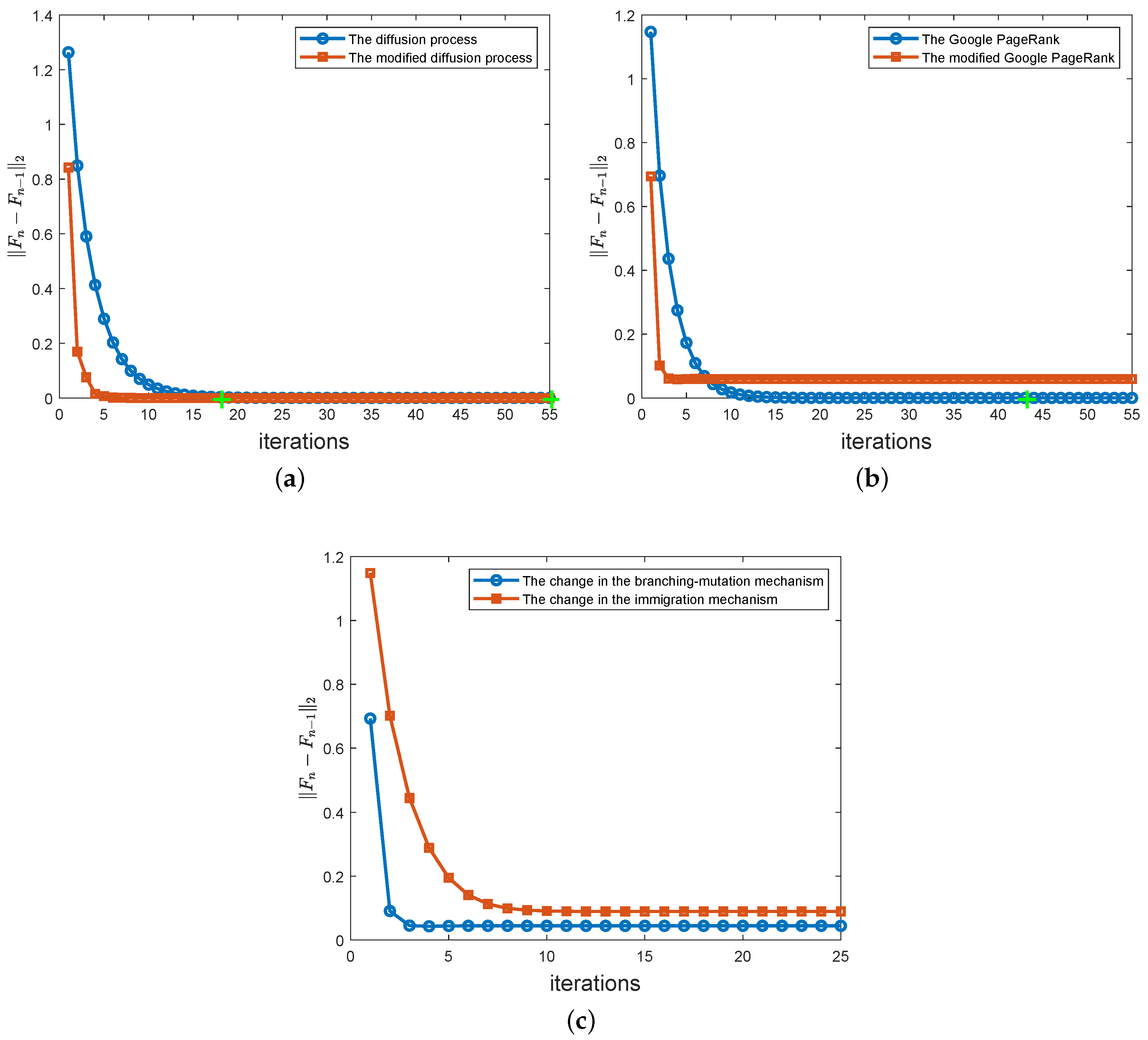
In MGWF with mutation, the initial branching law is $F_0=P$, such as the probabilities of the 1-type parent producing children of the $1,2,3$ types being $0,{\displaystyle \frac{2}{3}},{\displaystyle \frac{1}{3}}$, respectively. From Figure 3a, the unit time is divided into two phases in the n-th generation, the branching law in the branching phase is $F_n$, and the probability matrix of mutation in the mutation phase is $T=P$. The iterate result is $F_{n+1}=F_{n}T$. It is also found that the approximate stable state with the threshold of $1\times {10}^{-8}$ is basically reached after 88 iterations through simulation.

From the above description, we find that the model of MGWF with the mutation can intuitively explain the diffusion process better. Moreover, we make the probability matrix of mutation different in the odd iteration and even iteration mutation phases. For $\lambda \in (0,1)$, the specific iteration rule is

$$\begin{array}{c}\hfill F_{n+1}=\left\{\begin{array}{cc}{F}_{n}T,\hfill & \mathit{if}n\mathit{is}\mathit{odd};\hfill \\ F_n(\lambda T+(1-\lambda )I),\hfill & \mathit{if}n\mathit{is}\mathit{even}.\hfill \end{array}\right.\end{array}$$

(22)

To compare the difference in convergence speed between the modified version and the diffusion process, we take $\lambda ={\displaystyle \frac{1}{3}}$ and use $\parallel F_n-F_{n-1}{\parallel }_2$ to measure the convergence of $F_n$ with an accuracy of $1\times {10}^{-8}$. As shown in Figure 6a, for the same convergence accuracy, the modified version reaches an approximate stable state after 17 iterations, and its efficiency is significantly higher than that of the original diffusion process.

Example 5.

The Google PageRank system has the initial value $F_0=P$, the transition matrix P is given in Example 1, the probability matrix of the random jump is Y, and the iteration rule is $F_{n+1}=\alpha F_{n}P+(1-\alpha )Y$. We explain the Google PageRank system by MGWF with mutation and immigration with $\alpha =0.9$,

$$\begin{array}{c}\hfill Y=\left(\begin{array}{ccc}0& {\displaystyle \frac{2}{5}}& {\displaystyle \frac{3}{5}}\\ {\displaystyle \frac{1}{4}}& 0& {\displaystyle \frac{3}{4}}\\ {\displaystyle \frac{2}{5}}& {\displaystyle \frac{3}{5}}& 0\end{array}\right).\end{array}$$

The initial branching law is $\left(\begin{array}{cc}\alpha P& (1-\alpha )I\end{array}\right)$. The probability matrix of mutation is $\left(\begin{array}{c}P\\ Y\end{array}\right)$ in the mutation phase. In order to obtain the branching law of the $(n+1)$-th generation, it follows the result $\left(\begin{array}{cc}\alpha F_n& (1-\alpha )I\end{array}\right)\left(\begin{array}{c}P\\ Y\end{array}\right)$. It uses $\parallel F_n-F_{n-1}{\parallel }_2$ to measure the convergence of $F_n$ with the threshold of $1\times {10}^{-8}$. The Google PageRank system can reach this approximate stable state through 42 iterations.

While the random walk cannot explain the Google PageRank system, the Google PageRank system is perfectly explained by considering the immigration in the MGWF with mutation. Similar to the basic diffusion process, we propose a modified PageRank system by dividing each unit of time into two phases:

(i) 

It has some minor changes to the model of the Google PageRank system. We assume the branching law matrix is the same and the probability matrix of mutation is different in the odd iteration and even iteration mutation phases. In the odd iteration, the probability matrix of mutation is $\left(\begin{array}{c}P\\ Y\end{array}\right)$; in the even iteration, we change the probability matrix of mutation to $\left[\lambda \left(\begin{array}{c}P\\ Y\end{array}\right)+(1-\lambda )\left(\begin{array}{c}I\\ J\end{array}\right)\right]$. The iterative process is

$$\begin{array}{c}\hfill F_{n+1}=\left\{\begin{array}{cc}\left(\begin{array}{cc}\alpha F_n& (1-\alpha )I\end{array}\right)\left(\begin{array}{c}P\\ Y\end{array}\right),\hfill & \mathit{if}n\mathit{is}\mathit{odd};\hfill \\ \left(\begin{array}{cc}\alpha F_n& (1-\alpha )I\end{array}\right)\left[\lambda \left(\begin{array}{c}P\\ Y\end{array}\right)+(1-\lambda )\left(\begin{array}{c}I\\ J\end{array}\right)\right],\hfill & \mathit{if}n\mathit{is}\mathit{even}.\hfill \end{array}\right.\end{array}$$

(23)

where $\lambda \in (0,1)$, I is an identity matrix and

$$\begin{array}{c}\hfill J=\left(\begin{array}{ccc}0& {\displaystyle \frac{9}{10}}& {\displaystyle \frac{1}{10}}\\ {\displaystyle \frac{4}{5}}& 0& {\displaystyle \frac{1}{5}}\\ {\displaystyle \frac{3}{5}}& {\displaystyle \frac{2}{5}}& 0\end{array}\right).\end{array}$$

is another probability matrix of mutation in the immigration mechanism which is different from Y.

Let $\lambda ={\displaystyle \frac{3}{5}}$ and apply the revised Google PageRank system with N = 3 above. We find that the system reaches two different stable states in the seventh iteration and the eighth iteration, respectively, which makes the norm $\parallel F_n-F_{n-1}{\parallel }_2$ a fixed constant. The speed of reaching stability of the revised Google PageRank is faster than that of the original Google PageRank system. We will conduct an in-depth study on the relationship and the choice between the two stable states in the future.

The convergence behaviors of the Google PageRank system and the revised Google PageRank system is shown in Figure 6b. The modified version can reach stability within five iterations, but the Google PageRank needs about 10 iterations to reach stability.

(ii) 

We can make a couple of other changes to look at the branching–mutation mechanism and the immigration mechanism, whose change in mutation probability is responsible for the rate of convergence of $F_n$.

(a) 

(The change in the branching–mutation mechanism) In the odd and even iterations, the change in the branching–mutation mechanism is

$$\begin{array}{c}\hfill F_{n+1}=\left\{\begin{array}{cc}\left(\begin{array}{cc}\alpha F_n& (1-\alpha )I\end{array}\right)\left(\begin{array}{c}P\\ Y\end{array}\right),\hfill & \mathit{if}n\mathit{is}\mathit{odd};\hfill \\ \left(\begin{array}{cc}\alpha F_n& (1-\alpha )I\end{array}\right)\left(\begin{array}{c}(\lambda P+(1-\lambda \left)I\right)\\ Y\end{array}\right),\hfill & \mathit{if}n\mathit{is}\mathit{even}.\hfill \end{array}\right.\end{array}$$

(24)

We take $\lambda ={\displaystyle \frac{2}{5}}$ and find that the system reaches two different stable states in the seventh iteration and the eighth iteration, respectively.

(b) 

(The change in the immigration mechanism) In the odd and even iterations, a different probability matrix of immigration Y is selected respectively:

$$\begin{array}{c}\hfill F_{n+1}=\left\{\begin{array}{cc}\left(\begin{array}{cc}\alpha F_n& (1-\alpha )I\end{array}\right)\left(\begin{array}{c}P\\ Y\end{array}\right),\hfill & \mathit{if}n\mathit{is}\mathit{odd};\hfill \\ \left(\begin{array}{cc}\alpha F_n& (1-\alpha )I\end{array}\right)\left(\begin{array}{c}P\\ \lambda Y+(1-\lambda )J\end{array}\right),\hfill & \mathit{if}n\mathit{is}\mathit{even}.\hfill \end{array}\right.\end{array}$$

(25)

We take $\lambda ={\displaystyle \frac{2}{5}}$ and find that the system reaches two different stable states in the 11th iteration and the 12th iteration, respectively.

According to the iteration results of the (a) and (b) examples, it is found that changing the probability matrix of mutation in the branching–mutation mechanism is the key technique to improve the iteration speed. The convergence behaviors of (a) and (b) are shown in Figure 6c.

6. Conclusions

In this paper, we have connected the two seemingly unrelated fields of the diffusion and branching processes and established an explicit interpretation of the correspondence between the diffusion process and MGWF. Then, we focused on MGWF with the degenerated branching law and innovatively proposed the concept of particle mutation in MGWF with the degenerated branching law. Through the variation in MGWF, the vertices on the graph correspond to the types to explain the diffusion process, and the movement of particles can be observed more clearly from a longitudinal perspective. We divided each step of the diffusion process into two phases–the branching phase and the mutation phase—which not only interprets the mechanics more clearly but also removes the existing limitation that the transition probability P is dependent on the affinity matrix A. By extending MGWF with the concept of immigration, we further connected the MGWF model with the popular Google PageRank system, providing a new perspective to the latter as well. Both the diffusion process and the Google PageRank are well explained with the two-phase idea as shown in

Table 3. The diffusion process and the Google PageRank are explained with the two-phase idea.

Method	The Branching Law	The Probability of Mutation
Diffusion process	$F_n$	P
Google pagerank system	$\left(\begin{array}{cc}\alpha F_n& (1-\alpha )I\end{array}\right)$	$\left(\begin{array}{c}P\\ Y\end{array}\right)$

.

In the future, we will focus on the following directions:

•

From Table 3, we found that the existing improvements of the diffusion process are concentrated in the branching phase, that is, change the branching law by iteration. However, for the mutation phase, the mutation probability of all algorithms is constant. Therefore, in the future, we will pay more attention to changing the probability of mutation at each unit of time.

•

In Example 4, we found that the rate of convergence of the diffusion process was significantly accelerated after we made a slight change in the mutation probability. We will study how to change the probability of mutation to accelerate the rate of convergence.

•

In Example 5, after slight changes were made to the mutation probability of the Google PageRank system, we found that although the rate of convergence of the Google PageRank system was significantly accelerated, two stable states appeared. It will be of interest to study how to deal with two stable states.

References

- Yang, X.; Köknar-Tezel, S.; Latecki, L.J. Locally constrained diffusion process on locally densified distance spaces with applications to shape retrieval. In Proceedings of the IEEE Conference on Computer Vision & Pattern Recognition, Miami, FL, USA, 20–25 June 2009. [Google Scholar]
- Bai, X.; Yang, X.; Latecki, L.J.; Liu, W.; Tu, Z. Learning Context-Sensitive Shape Similarity by Graph Transduction. IEEE Trans. Pattern Anal. Mach. Intell. 2010, 32, 861–874. [Google Scholar] [CrossRef] [PubMed]
- Egozi, A.; Keller, Y.; Guterman, H. Improving shape retrieval by spectral matching and meta similarity. IEEE Trans. Image Process. 2010, 19, 1319–1327. [Google Scholar] [CrossRef] [PubMed]
- Wang, B.; Tu, Z. Affinity learning via self-diffusion for image segmentation and clustering. In Proceedings of the 2012 IEEE Conference on Computer Vision and Pattern Recognition, Providence, RI, USA, 16–21 June 2012. [Google Scholar]
- Donoser, M.; Bischof, H. Diffusion Processes for Retrieval Revisited. In Proceedings of the IEEE Conference on Computer Vision and Pattern Recognition, Portland, OR, USA, 23–28 June 2013. [Google Scholar]
- Li, Q.; Liu, W.; Li, L. Affinity learning via a diffusion process for subspace clustering. Pattern Recognit. 2018, 84, 39–50. [Google Scholar] [CrossRef]
- Donoser, M. Replicator Graph Clustering. In Proceedings of the British Machine Vision Conference, Bristol, UK, 9–13 September 2013. [Google Scholar]
- Chen, S.; Zheng, L.; Hu, X.; Zhou, P. Discriminative saliency propagation with sink points. Pattern Recognit. 2016, 60, 2–12. [Google Scholar] [CrossRef]
- Lu, S.; Mahadevan, V.; Vasconcelos, N. Learning optimal seeds for diffusion-based salient object detection. In Proceedings of the IEEE Conference on Computer Vision and Pattern Recognition, Columbus, OH, USA, 23–28 June 2014; pp. 2790–2797. [Google Scholar]
- Yang, X.; Prasad, L.; Latecki, L.J. Affinity Learning with Diffusion on Tensor Product Graph. IEEE Trans. Pattern Anal. Mach. Intell. 2013, 35, 28–38. [Google Scholar] [CrossRef] [PubMed]
- Elhamifar, E.; Vidal, R. Sparse Subspace Clustering: Algorithm, Theory, and Applications. IEEE Trans. Pattern Anal. Mach. Intell. 2012, 35, 2765–2781. [Google Scholar] [CrossRef] [PubMed]
- Berzunza, G. On scaling limits of multitype Galton-Watson trees with possibly infinite variance. arXiv 2016, arXiv:1605.04810. [Google Scholar] [CrossRef]
- Miermont, G. Invariance principles for spatial multitype Galton-Watson trees. Ann. Inst. Henri Poincaré Probab. Stat. 2008, 44, 1128–1161. [Google Scholar] [CrossRef]
- de Raphelis, L. Scaling limit of multitype Galton-Watson trees with infinitely many types. Ann. Inst. Henri Poincaré Probab. Stat. 2017, 53, 200–225. [Google Scholar] [CrossRef]
- Duquesne, T. A limit theorem for the contour process of condidtioned Galton–Watson trees. Ann. Probab. 2003, 31, 996–1027. [Google Scholar] [CrossRef]
- Le Gall, J.F.; Duquesne, T. Random Trees, Levy Processes, and Spatial Branching Processes. Asterisque 2002, 281, 30. [Google Scholar]
- Chaumont, L.; Nguyen, T.N.A. On mutations in the branching model for multitype populations. Adv. Appl. Probab. 2018, 50, 543–564. [Google Scholar] [CrossRef]
- Cheek, D.; Antal, T. Mutation frequencies in a birth–death branching process. Ann. Appl. Probab. 2018, 28, 3922–3947. [Google Scholar] [CrossRef]
- Lax, P.D. Linear Algebra and Its Applications; John Wiley & Sons: Hoboken, NJ, USA, 2007; Volume 78. [Google Scholar]
- Haggstrom, O. Finite Markov Chains and Algorithmic Applications; Cambridge University Press: Cambridge, UK, 2002; Volume 52. [Google Scholar]
- Seneta, E. On the supercritical Galton-Watson process with immigration. Math. Biosci. 1970, 7, 9–14. [Google Scholar] [CrossRef]
- Seneta, E. A note on the supercritical Galton-Watson process with immigration. Math. Biosci. 1970, 6, 305–311. [Google Scholar] [CrossRef]
- Liu, J.N.; Zhang, M. Large deviation for supercritical branching processes with immigration. Acta Math. Sin. Engl. Ser. 2016, 32, 893–900. [Google Scholar] [CrossRef]
- Sun, Q.; Zhang, M. Harmonic moments and large deviations for supercritical branching processes with immigration. Front. Math. China 2017, 12, 1201–1220. [Google Scholar] [CrossRef]