Abstract
High-dimensional sparse matrix data frequently arise in various applications. A notable example is the weighted word–word co-occurrence count data, which summarizes the weighted frequency of word pairs appearing within the same context window. This type of data typically contains highly skewed non-negative values with an abundance of zeros. Another example is the co-occurrence of item–item or user–item pairs in e-commerce, which also generates high-dimensional data. The objective is to utilize these data to predict the relevance between items or users. In this paper, we assume that items or users can be represented by unknown dense vectors. The model treats the co-occurrence counts as arising from zero-inflated Gamma random variables and employs cosine similarity between the unknown vectors to summarize item–item relevance. The unknown values are estimated using the shared parameter alternating zero-inflated Gamma regression models (SA-ZIG). Both canonical link and log link models are considered. Two parameter updating schemes are proposed, along with an algorithm to estimate the unknown parameters. Convergence analysis is presented analytically. Numerical studies demonstrate that the SA-ZIG using Fisher scoring without learning rate adjustment may fail to find the maximum likelihood estimate. However, the SA-ZIG with learning rate adjustment performs satisfactorily in our simulation studies.
Keywords:
high-dimensional co-occurrence matrix; matrix factorization; zero-inflated Gamma regression; Adam; recommender system MSC:
62-08; 62J99
1. Introduction
Matrix factorization is a fundamental technique in linear algebra and data science, widely used for dimensionality reduction, data compression, and feature extraction. Recent research expands its use in various fields, including recommendation systems (e.g., collaborative filtering), bioinformatics, and signal processing. Researchers are actively pursuing new types of factorizations. In their effort to discover new factorizations and provide a unifying structure, ref. [1] list 53 systematically derived matrix factorizations arising from the generalized Cartan decomposition. Their results apply to invertible matrices and generalizations of orthogonal matrices in classical Lie groups.
Nonnegative matrix factorization (NMF) is particularly useful when dealing with non-negative data, such as in image processing and text mining. Ref. [2] survey existing NMF methods and their variants, analyzing their properties and applications. Ref. [3] present a comprehensive survey of NMF, focusing on its applications in feature extraction and feature selection. Ref. [4] summarize theoretical research on NMF from 2008 to 2013, categorizing it into four types and analyzing the principles, basic models, properties, algorithms, and their extensions and generalizations.
There are many advances aimed at developing more efficient algorithms tailored to specific applications. One prominent application of matrix factorization is in recommendation systems, particularly for addressing the cold-start problem. In recommender systems, matrix factorization models decompose user–item, user–user, or item–item interaction matrices into lower-dimensional latent spaces, which can then be used to generate recommendations.
Ref. [5] summarizes the literature on recommender systems and proposes a multifaceted collaborative filtering model that integrates both neighborhood and latent factor approaches. Ref. [6] develop a matrix factorization model to generate recommendations for users in a social network. Ref. [7] proposes a matrix factorization model for cross-domain recommender systems by extracting items from three different domains and finding item similarities between these domains to improve item ranking accuracy.
Ref. [8] develop a matrix factorization model that combines user–item rating matrices and item–side information matrices to develop soft clusters of items for generating recommendations. Ref. [9] propose a matrix factorization that learns latent representations of both users and items using gradient-boosted trees. Ref. [10] provide a systematic literature review on approaches and algorithms to mitigate cold-start problems in recommender systems.
Matrix factorization has also been used in natural language processing (NLP) in recent years. Word2Vec by [11,12] marks a milestone in NLP history. Although no clear matrices are presented in their study, Word2Vec models the co-occurrence of words and phrases using latent vector representations via a shallow neural network model. Another well-known example of matrix factorization in NLP is the word representation with global vectors (GloVe) by [13]. They model the co-occurrence count matrix of words using cosine similarity of latent vector representations via alternating least squares. However, practical data may be heavily skewed, making the sum or mean squared error unsuitable as an objective function. To address this, ref. [13] utilize weighted least squares to reduce the impact of skewness in the data. Manually creating the weight is difficult to make it work well for real data. In GloVe training, the algorithm is set to run a fixed number of iterations without another convergence check. Here, we consider using the likelihood principle to model the skewed data matrix.
In this paper, our goal is to model non-negative continuous sparse matrix data from skewed distributions with an abundance of zeros but lacking covariate information. We are particularly interested in zero-inflated Gamma observations, often referred to as semi-continuous data due to the presence of many zeros and the highly skewed distribution of positive observations. Examples of such data include insurance claim data, household expenditure data, and precipitation data (see [14]). Ref. [15] study and simulate data using actual deconvolved calcium imaging data, employing a zero-inflated Gamma model to accommodate spikes of observed inactivity and traces of calcium signals in neural populations. Ref. [16] examine the amount of leisure time spent on physical activity and explanatory variables such as gender, age, education level, and annual per capita family income. They find that the zero-inflated Gamma model is preferred over the multinomial model. Beyond Gamma distribution, Weibull distribution can also model skewed non-negative data. Unfortunately, when the shape parameter is unknown, the Weibull distribution is not a member of the exponential family. Further, the alternating update is not suitable because its sufficient statistics is not linear in the observed data. A different estimation procedure will need to be developed if Weibull distribution is used. The Gamma distribution not only is a member of the exponential family, but its sufficient statistic is also linear in the observed data. This gives solid theoretical ground for alternating update to find a solution. Section 5 explains more details in this regard.
In all the aforementioned examples, there are explicitly observed covariates or factors. Furthermore, the two parts of the model parameters are pendicular to each other, allowing model estimation by fitting two separate regressions: binomial regression and Gamma regression. Unfortunately, such models cannot be applied to user–item or co-occurrence count matrix data arising from many practical applications. Examples include user–item or item–item co-occurrence data from online shopping platforms and co-occurring word–word pairs in sequences of texts. One reason is the absence of observed covariates. Additionally, the mechanism that leads to the observed data entries in the data matrix for the binomial and Gamma parts may be of the same nature, making it more appropriate to utilize shared parameters in both parts of the model. Therefore, in this paper, we consider shared parameter modeling of zero-inflated Gamma data using alternating regression. We consider two different link functions for the Gamma part: canonical link and log link.
We believe that our study is the first that utilizes a shared parameter likelihood for zero-inflated skewed distribution to conduct matrix factorization. The alternating least squares (ALS) shares a similar spirit as our SA-ZIG in terms of alternately updating parameters. Most matrix factorization methods in the literature involving ALS are adding an assumption without realizing it. In order for ALS to be valid, the data need to have constant variance. This is because the objective function behind the ALS procedure is the mean squared error, which gives equal emphasis to all observations regardless of how big or small their variations are. If the variations for different observations are drastically different, it is unfair to treat the residuals equally. The real data in the high-dimensional sparse co-occurrence matrix are often very skewed with a lot of zeros and do not have constant variance. The contribution of this paper is the SA-ZIG model that models the positive co-occurrence data with Gamma distribution and attributes the many zeros in the data as being from a Bernoulli distribution. Shared parameters are used in both the Bernoulli and Gamma parts of the model. The latent row and column vector representations in matrix decomposition can be thought of as missing values that have some distributions relying on a smaller set of parameters. Estimating the vector representation for the rows relies on the joint likelihood of the observed matrix data and the missing vector representation for the columns. Due to missingness, the estimation of row vector representations is transformed to using conditional likelihood of the observed data given the column vector representations, and vice versa. This alternating update in the end gives the maximum likelihood estimate if the sufficient statistic for the column vector representation is linear in the observed data and the row vector representations. Both ALS and our SA-ZIG rely on this assumption to be valid.
The remainder of this paper is structured as follows. Section 2 outlines the fundamental framework of the ZIG model. Section 3 focuses on parameter estimation within the SA-ZIG model using the canonical link. Section 4 addresses parameter estimation for the scenario involving the log link in the Gamma regression component. Convergence analysis is presented in Section 5. Section 6 details the SA-ZIG algorithms incorporating learning rate adjustments. Section 7 presents the experimental studies. Finally, Section 8 concludes the paper by summarizing the research findings, contributions, and limitations.
3. ZIG Model with Canonical Links
In this section, we consider the case with canonical links, i.e., the Bernoulli part uses logit function and the Gamma part uses negative inverse link. Using the canonical link with generalized linear models enjoys the benefit that the score equations are a function of sufficient statistics. Here, we consider parameter estimation under the canonical links. The negative inverse link has difficulty interpreting model parameters and also has some restrictions in terms of the support of the link function, which does not match the positive value of Gamma distribution. More details can be seen as we introduce the model.
Recall that the the log likelihood and the link function for the logistic part on the row of data are
where and are unknown parameters while treating and as fixed. The log likelihood and the negative inverse link function for the Gamma part on the row of data are
The log likelihood function for the row of data is
To obtain partial derivatives, we write as follows:
The inverse logit and its partial derivative w.r.t. are
Therefore, the first-order partial derivatives can be summarized as
The negative second-order partial derivatives and their expectations are the same and are given below:
Now, consider the second component of the log likelihood from the ith row of data
The first-order partial derivatives for the are
The second-order partial derivatives and their negative expectations are
All of the aforementioned formulae work with the row of data. When we combine the log likelihood from different rows of data, other rows do not contribute to the partial derivative with respect to . That is,
As a result, the estimation of the components in does not need to be performed simultaneously. Instead, we can cycle through the estimation of , for , one by one iteratively. After is updated, the estimated value of is used to update .
The first part of the alternating regression has the following updating equation based on the Fisher scoring algorithm:
For each i and t, this update requires the value of and their score equations and information matrix at the iteration. One iteration alone here is not taking advantage of the data because retrieving the row of data takes a significant amount of time when the dimension of the data matrix is huge. Therefore, for each row of data retrieved, it is better to update a certain number of times. Specifically, the is updated again and again in a loop of E epochs and the updated values are used to recompute the score equations and information matrix, all of which are used for next epoch’s update. After all epochs are completed, takes the value of at the end of all iterations from E epochs based on the updating formula below:
This inner loop of updates makes good use of the already loaded data to refine the estimate of so that the end estimate is closer to its MLE when the same current values are used. Note that the updated in each epoch from (20) leads to changes in the score equations and Fisher information matrix, whose update will in turn result in a better estimate of . Such multiple rounds of updates in (20) reduce the variation of update in when we go through many iterations based on Equation (19). It effectively reduces the number of times to retrieve the data. Below are the formulae involved in the updating equations:
with
where these partial derivatives are the , , , and evaluated at and using formulae in (8) and (12), and
where the expectations are based on Formulae (9), (10), (13)–(15) evaluated at and if it is in the outer loop of the update and using the values of and when it is in the inner loop of updates.
This concludes the first part of the alternating ZIG regression. It gives an iterative update of while is fixed. After we finish updating all ’s, we move on to treat the as fixed to estimate .
Starting with , we consider the partial derivatives with respect to while holding fixed. The derivations are similar to those for but still we list them for clarity. Note that
The first-order partial derivatives regarding are
The negative second derivatives and their expectations are
The first-order partial derivatives of the second component are .
The negative second-order partial derivatives and their expectations are
Therefore, the other side of the updating equation for the alternating ZIG regression based on the Fisher scoring algorithm is
Again, for each j and iteration number t, this equation is iterated for a certain number of epochs to obtain a refined estimate of based on the current value without having to reload the data. The quantities in the updating equation are listed below.
with
where these partial derivatives are , , , and evaluated at and , and
The expectations involved in the above formulae were using at the iteration and the current values if it is in the outer loop of the update and using the values of and when it is in the inner loop of updates.
All of the formulae above assume the parameter is known. When it is not known, the parameter can be estimated with MLE, bias corrected MLE, or moment estimator. Simulation studies in [21] suggested that when the sample size is large, all the estimators perform similarly but the moment estimator has the advantage of being easy to compute. If the sample size is medium, then bias corrected MLE is better.
The canonical link for the Gamma regression part could encounter problems. Recall that the canonical link for the Gamma regression is . The left-hand side of the equation is required to be negative because the support of the Gamma distribution is (0, . However, the right-hand side of the equation could freely take any value in . Due to this conflict in natural parameter space and the range of the estimated value, the likelihood function sometimes could become undefined because appears in it but cannot be evaluated for negative (see Equation (11)).
4. Using Log Link for Gamma Regression
In this section, we consider using the log link to model the Gamma regression part while maintaining the logistic regression part. The settings of the two-part model are similar to those in Section 3 except that modifying the link function from canonical to log link changes the score equations and the Hessian matrix.
For updating formulae on the model parameters based on Fisher scoring algorithm, the first-order and second-order partial derivatives of remain the same as in (8)–(10) because the new link function does not appear in the Bernoulli part. Now consider the second component of the log likelihood , which was given in (5). In this section, denote as in the previous subsection. Then, the log likelihood of the ith row of non-zero observations in the co-occurrence matrix, corresponding to the Gamma distribution, can be expressed as
The equations below give the first-order partial derivatives of with respect to the parameters and .
To obtain the second-order partial derivatives, first note that
Then, the second-order partial derivatives and their negative expectations which are components of the Fisher information matrix can be derived as
The first part of the alternating regression has the following updating equation based on the Fisher scoring algorithm:
The updating equation in (29) is iterated E epochs, say E equals 20, for the same i and t, where t is the iteration number. The multiple epochs here allow the estimate of to get closer to its MLE for given current value as the score equations and information matrix are also updated with the estimated parameter value. There is no need to have too many epochs because the parameter is not the true value yet and still needs to be estimated later. Below are the formulae involved in the updating equations:
with
where these partial derivatives are , , , and evaluated at and using Equations (8) and (25), and
The expectations involved in the above formulae were given in (9)–(10) and (26)–(28) except that the parameters are using the current values and at the iteration if it is in the outer loop of the update and using the values of and when it is in the inner loop of updates.
The aforementioned equations are used in updating the part of the alternating ZIG regression. Now, consider the other side of the alternating ZIG regression in which updates are performed for while holding fixed. First, consider the first-order partial derivatives
The first-order partial derivatives of are
The second-order partial derivatives , , and their expectations are same as in the canonical link case, which are given in Equations (21)–(23). Additionally,
Next, consider the first-order partial derivatives of the second component
To derive the second-order partial derivatives, note that two frequently used terms are
Using the two terms, the second derivatives can be written as
Therefore, the updating equations for based on the Fisher scoring algorithm are
The updating Equation (30) is in the outer loop of iterations and the iterations in (31) are in the inner loop of epochs for the same j and t. The quantities involved are
with
where these partial derivatives are derivatives , , , and
evaluated at and during the outer loop of iterations and at and during the inner loop of iterations.
5. Convergence Analysis
In this section, we discuss the convergence behavior of the algorithm analytically. Our algorithm contains two components: a logistic regression part and a Gamma regression part. If these two components’ parameter estimations were independent of each other, then it is the situation of the standard Generalized Linear Model (GLM) in each part. In our model, the two components’ estimation cannot be separated but the two components in the log likelihood are additive. Hence, the convergence behavior in one component standard GLM case is still relevant. In this section, we first talk about the convergence behavior in the standard case, as this case applies to the situation when we hold the fixed while estimating or vice versa.
In the standard GLM setting, most of the parameter estimation converges pretty fast. There are also abnormal behaviors that could happen such as when the estimated model component gets out of the valid range of the distribution. For example, in the Gamma regression, if the canonical link (negative inverse) is used, the estimated mean may become negative every now and then even though the distribution requires a positive mean. Refs. [22,23,24] presented conditions for the existence of MLE in logistic regression models. They proved in the non-trivial case that if there is overlap in the convex cones generated by the covariate values from different classes, the maximum likelihood estimates of the regression parameters exist and are unique. On the other hand, if the convex cones generated by the covariates in different classes have complete separation or quasi complete separation, then the maximum likelihood estimates do not exist or are unbounded. Generally, they recommended inserting a stopping rule if complete separation is found or restarting the iterative algorithm with standardized observations (to have mean 0 and variance 1) if quasi complete separation is found. Ref. [24] also recommended a procedure to check the conditions. For quasi complete separation, the estimation process diverges at least at some points. This makes the estimated probability of belonging to the correct class grow to one. Therefore, ref. [24] recommended checking the maximum predicted probability for each data point at the iteration. If the maximum probability is close to 1 and is bigger than previous iterations’ maximum probability, there are two possibilities for which this could happen. They suggested initially printing a warning but continue the iteration because the data point is likely to be an outlier observation in its own class and there is overlap in the two convex cones. In this case, the MLE exists and is unique so the algorithm should be allowed to continue. The other possibility is that there is quasi complete separation in the data. In this case, the process should be stopped and rerun with the observation vectors standardized with zero mean and unit variance.
Ref. [24] also stated that the difficulties associated with complete and quasi complete separation are small sample problems. With large sample size, the probability of observing a set of separated data points is close to zero. Complete separation may occur with any type of data but it is unlikely that quasi complete separation will occur with truly continuous data.
Ref. [25] illustrated the non-convergence problem with a Poisson regression example. The author proposed a simple solution and implemented it in the R package, version 1.2.1. Specifically, if the iteratively reweighted least squares (IRLS) procedure produces either an infinite deviance or predicted values which fall within an invalid range, then the amount of update of the parameter estimates is repeatedly halved until the update no longer shows the behavior. Moreover, it produced a further step-halving, which checks that the updated deviance is making a reduction compared to that in the previous iteration. If it did not show the reduction, it triggers the step-halving to make the algorithm monotonically reduce the deviance.
Based on the aforementioned studies illustrating the standard case of GLM convergence behavior, we analytically present the convergence behavior of our alternating ZIG regression. For further discussion, we first specify our convex cones. Recall that serves as data when we estimate . In our context, the convex cones are defined through , while we estimate and through while we estimate . That is, for estimating , the convex cones are
For estimating the , the convex cones are denoted as and , respectively.
Firstly, we consider the case that either complete separation or quasi complete separation exists in the data. We discuss the estimation of while holding fixed.
Suppose there exists complete separation or quasi separation in and . That is, , , and . Also, suppose and . Then, there exists a vector direction such that for and for . (Note: This vector can be taken to be the perpendicular direction to a vector that lies in between and but does not belong to either or .) Let be the log likelihood of the Bernoulli part when the model parameters are updated toward direction by k unit. That is, the original log likelihood and the updated are as follows:
- For . Hence, as k increases to ∞, increases toward 1. This implies increases toward 0.
- For , . Hence, as k increases to ∞, decreases toward 0. This implies increases toward 0.
Putting the two pieces together, we know that as k increases, increases for any given . Therefore, the maximum cannot be reached until k is ∞. This means the MLE does not exist or the solution set is unbounded for the current value of . This perspective can be also seen by looking at the partial derivative of with respect to k. Note that
Since when , we know the first term is non-negative. Similarly, when implies the second term is non-negative. Therefore, the partial derivative of is non-negative. This indicates that the gradient of is positive unless . Therefore, there is no solution for except the trivial solution in binomial regression alone. Of course, this is not exactly our case because we still have the Gamma regression component to be considered together.
Now consider the component with its first- and second-order derivatives with respect to k.
where . Note that
where is the standardized Gamma random variable that has mean 0 and variance 1 because the term is the mean of and is the shape parameter. Further,
The negativity of the second-order derivative implies that is concave.
Gathering the partial derivatives from both and together, we obtain the partial derivative of
From the above discussion, the first two terms in (35) corresponding to are greater than 0. The is centered at zero and has variance 1. Therefore, in order for the MLE to exist, the sum of must cancel the total value of and the positive term . If the shape parameter of Gamma distribution is small, the distribution is highly skewed with a long right tail. In this case, there are more observations having values less than its mean. However, a small shape parameter also makes small such that the may dominate, and hence, the entire partial derivative is greater than zero. When the shape parameter is large, the Gamma random variables are approximately normally distributed. In this case, the observations are symmetrically located on either side of its mean. This makes the number of observations satisfying and roughly equal. Consequently, the is close to zero. Then, there are no extra values left to neutralize . As a result, regardless of whether the shape parameter is large or small, when complete separation or quasi complete separation holds, it is highly likely that the MLE does not exist. When the shape parameter is intermediate such that the Gamma distribution is still skewed, the more values of Gamma observations less than its mean might allow to cancel all other positive terms. This is the case that there could be a solution for .
Next, consider the case that there is overlap in the two convex cones and (i.e., there is neither complete separation nor quasi complete separation in the data). Recall that the ZIG model is a two-part model with a Bernoulli part and a Gamma part. The log likelihood function corresponding to the Bernoulli part can be shown to be strictly concave in . This is because the first component in is an affine function of (see Equation (7) for the expression of ), which is both convex and concave, if we hold and fixed. The second component is strictly concave, as its second derivative is less than 0, as shown below.
Thus, the log likelihood corresponding to the Bernoulli part is strictly concave.
Now, consider the log likelihood corresponding to the Gamma part in (24). We only need to consider the summation over the last two terms and because the other terms do not involve the regression parameters, where . Note that is an affine function of , which is both convex and concave and is convex if is convex (see ref. [26]). This leads to the term being strictly concave in . Hence, we have the strictly concave in . Combining the two concave components and , we know that the entire log likelihood for the row is a strictly concave function with respect to the parameter being estimated for any row i. Additionally, there is overlap in the two convex cones. Therefore, for any direction in the overlapping area of the convex cones, updating the parameter along that direction will lead to the two components of in Formula (34) being of opposite sign to each other. In this case, has a unique minimum when there is neither complete separation nor quasi complete separation in and . Similar arguments apply when we estimate while holding fixed. That is, a unique MLE of exists when there is neither complete separation nor quasi complete separation in and . This means that the alternating procedure will find the MLE of when is fixed and will find the MLE of when is fixed in this non-separation scenario.
Next, we consider the convergence behavior for the estimation of without fixing the value of . For estimating , consider the complete data . The entire matrix is missing. Due to too many missing values, a logical approach is to regard the as randomly drawn from a distribution which has relatively few parameters. Assume the distribution of is in the exponential family.
Let be the unconditional density of the complete data and be the conditional density given . Denote the marginal density of given as . In the next few paragraphs, we explain that the alternating updates in ZIG leads ultimately to a value of that maximizes .
For exponential families, the unconditional density and conditional density both have the same natural parameter and the same sufficient statistic except that they are defined over different sample spaces versus . We can write and in general exponential family format as
where
Then, . The first- and second-order derivatives of are
where and are the expectation and variance under the complete data likelihood from and . And and are the conditional expectation and variance of the sufficient statistics. is the expected value of the conditional covariance matrix when has sampling density . The last equality of both equations assumes the order of expectation and derivative can be exchanged. The previous equation means the derivative of the log likelihood is the difference between the conditional and unconditional expectation of the sufficient statistics.
Meanwhile, the updating equation based on the Fisher scoring algorithm can be written as
where in the limit, , for some , which leads to or at .
The complete data log likelihood based on the joint distribution of can be written as , where is defined in the end of Section 2, and is the probability density function of given . We know is also a member of the exponential family. Assume its sufficient statistics are linear in . Given , the observed data likelihood based on contains the Bernoulli and Gamma parts, in which the sufficient statistic for is linear in . Then, the sufficient statistics for the complete data problem are linear in the data and . In this case, calculating is equivalent to a procedure which first fills in the individual data points for and then computes the sufficient statistics using filled-in values. With the filled-in value for , the computation of the estimator for follows the usual maximum likelihood principle. This results in iterative update of and back and forth. Essentially, the problem is a transformation from an assumed parameter-vector to another parameter-vector that maximized the conditional expected likelihood.
One of the difficulties in the ZIG model is that the parameterization allows arbitrary orthogonal transformations on both and without affecting the value of the likelihood. Even for cases where the likelihood for the complete data problem is concave, the likelihood for the ZIG may not be concave. Consequently, multiple solutions of the likelihood equations can exist. An example is a ridge of solutions corresponding to orthogonal transformations of the parameters.
For complete data problems in exponential family models with canonical links, the Fisher scoring algorithm is equivalent to the Newton–Raphson algorithm, which has a quadratic rate of convergence. This advantage is due to the fact that the second derivative of the log-likelihood does not depend on the data. In these cases, the Fisher scoring algorithm has a quadratic rate of convergence when the starting values are near a maximum. However, we do not have the complete data and when estimating . Fisher scoring algorithms often fail to have quadratic convergence in incomplete data problems, since the second derivative often does depend upon the data. Further, the scoring algorithm does not have the property of always increasing the likelihood. It could in some cases move toward a local maximum if the choice of starting values is poor.
In summary, we conclude that our alternating ZIG regression has an unique MLE in each side of the regressions when either or stays fixed and the algorithm converges when there is overlap in data. The data refer to while we estimate and refer to while we estimate . When there is overlap in data, both and are concave functions with unique maximum. However, when there is complete separation or quasi complete separation, the alternating ZIG regression will fail to converge with high chance. This is because the first-order partial derivative of is non-negative and increases with k. Even though the component is a well-behaved concave curve, the entire log likelihood, unfortunately, may not have MLE exist or the solution set may be unbounded especially when the Gamma observations have large or too small shape parameter. The overall convergence behavior for estimating without holding fixed can treat as missing data. The alternating update ultimately finds the maximum likelihood estimate of based on the sampling distribution of the observed matrix if the solution is in the interior of the parameter space. This requires the joint distribution of and to be in the exponential family with sufficient statistic that is linear in and .
6. Adjusting Parameter Update with Learning Rate
In the convergence analysis section, our discussion is based on holding either or fixed while estimating the other one. The Fisher scoring algorithm is a modified version of Newton’s method. In general, Newton’s method solves by numerical approximation. This algorithm starts with an initial value and computes a sequence of points via . Newton’s method converges fast because the distance between the estimate and its true value shrinks quickly such that the distance in the next step of iteration is asymptotically equivalent to the squared distance in the previous iteration. That is, Newton’s method has quadratic convergence order (cf. [27] p. 29 and [28]). This convergence order holds when the initial value of the iteration is in the neighborhood of the true value and the third derivative is continuous and is non-zero.
The Fisher scoring algorithm is slightly different from Newton’s method. In the Fisher scoring algorithm, we replace the by its expected value. This algorithm is asymptotically equivalent to Newton’s method and therefore enjoys the same asymptotic property such as consistency of the estimate of the parameter. As sample size becomes large, the convergence order increases [28]. It has some advantages over Newton’s method in that the expected value of the Hessian matrix is positive definite which guarantees the update is uphill toward the direction of maximizing the log likelihood function assuming that the model is correct and the covariates are true explanatory variables.
As the Fisher scoring algorithm assumes that is the true value when we estimate or vice versa, there could be complications when the parameter being fixed is not equal to the true parameter value. To see this point, note that our updating equations are all written in the context of using the Fisher scoring algorithm, which relies on the expectation of the Hessian matrix using correct distribution at the true parameter value. In particular, the algorithm uses as a fixed value while estimating . The resulting estimate of determines the distribution because the distribution is a function of and . When the parameter is being fixed at a value far from its true value during the intermediate steps, the distribution is wrong even though it is in the right family. The consequence of using a wrong distribution to compute the expectation of the Hessian matrix could lead to a sequence of parameter updates that converges to a limiting value unequal to the true parameter [28]. In this case, the algorithm might diverge. Our simulation study in later section confirms this point.
To avoid this parameter update divergence problem, we introduce learning rate adjustment so that the change in parameter estimate is scaled by , where is a small constant learning rate such as 0.1 or 0.01, and t is the iteration number. That is, the general updating formula is and the adjustment is applied to both inner loop and outer loop iterations. The algorithm follows the same work flow as those listed in Algorithm 1 except that the epoch update in the inner loop (Algorithm 2) is replaced with the Algorithm 3 using the learning rate adjustment . How we decide to use this learning rate adjustment comes from modifying the popularly used adaptive moment estimation (Adam) and the stochastic gradient descent. In the stochastic gradient descent, the parameter update has learning rate adjustment to make small moves so that it compensates for the random nature of selecting only one observation to compute the gradient. Specifically, given parameters and a gradient function evaluated at one randomly selected observation , the update is based on formula , where satisfies and . The corresponds to our . However, our parameter update does not use just one . Instead, all were used in computing the gradient and the information matrix. Given parameters and a loss function at the training iteration, the Adam update takes the form , where and are the exponential moving average of the gradients and the second moments of the gradients in the past iterations, respectively, and is a small scalar (e.g., ) used to prevent division by 0. Our use of the Fisher information should provide a better mechanism than Adam’s exponential moving average of second moments to achieve the effect of increasing the learning rate for sparser parameters and decreasing the learning rate for ones that are less sparse. This is because Adam only uses the diagonal entries of and ignores the covariance between the estimated parameters existing in the off-diagonal entries. Refs. [29,30] both pointed out that Adam may not converge to optimal solutions even for some simple convex problems, although it is overwhelmingly popular in machine learning applications.
Using the learning rate adjustment makes smaller steps in each update before changing directions. This learning rate adjustment turns out to be crucial. The simulation study in the next section examines the effect of the learning rate adjustment.
| Algorithm 1 SA-ZIG regression |
|
| Algorithm 2 Epoch update in inner loop of Algorithm 1 without learning rate adjustment |
|
| Algorithm 3 Updating equations in SA-ZIG regression with learning rate adjustment |
|
7. Numerical Studies
7.1. A Simulation Study with ZIG Using Log Link
In this section, we present a simulation study to assess the performance of the alternating ZIG regression. We found through some experiments that data generation has to be very careful because the mean of the Gamma distribution was given by . When we randomly generate the ’s and ’s independently from Uniform distribution with each of them having dimension 50, their dot product could easily become so large that exponentiated value and the variance of the distribution (∝ ) become infinity or undefined. Keeping this point in mind, we generate the data as follows:
- The ’s were generated independently from Uniform (−0.25, 0.25) with seed 99, and . Set .
- The , and . That is, .
- The ’s and ’s were generated independently from Uniform (0, 0.05) with seed 97 and 96, respectively, .
- The ’s and ’s were generated independently from Uniform (0.1, 0.35) with seed 1 and 2, respectively, .
- The success probability of positive observations was calculated as , where is based on the logit Formula (2).
- Generate independently from the Bernoulli distribution with success probability , and .
- If , set . Otherwise, generate from the Gamma distribution with mean and shape parameter , where is computed based on Formula (4) for and .
The matrix containing , , is the data we used for the alternating ZIG regression. With the generated data matrix , we applied our algorithm to the data with two different sets of initial values for the unknown parameters. One setting is to check whether the algorithm would perform well when the parameter estimation is less difficult when part of the parameters was initialized with true values. The other setting demands more accurate estimation in both and in the right direction.
In Setting 1, we set all the parameters’ initial values equal to their true values except for . The initial values of ’s were randomly generated from Uniform (−0.25, 0.25) with seed number 98. Even though initial values of and were set to be equal to the true values, the algorithm was not aware of this and these parameters were still estimated along with .
In Setting 2, we generated the initial values for all the parameters randomly as follows:
- ’s initial values were generated independently from Uniform (−0.25, 0.25) with dimension 300 by 50 and seed 102.
- ’s initial values were generated independently from Uniform (−0.25, 0.25) with dimension 300 by 50 and seed 103.
- ’s and ’s initial values were generated independently from Uniform (0, 0.05) with seed 104 and 105, respectively, .
- ’s and ’s were independently generated from Uniform (0.1, 0.35) with seed 106 and 107, respectively, .
We consider update both with learning rate adjustment (Algorithm 3) and without learning rate adjustment (Algorithm 1).
The results of Setting 1 are presented in Table 1 and Figure 1. We can see in Figure 1 that even though the norm of the score vectors went up after initial reduction, the loss function (i.e., the negative log-likelihood) consistently decreases as the iteration number increases. In the last five iterations, the algorithm with no learning rate adjustment (Algorithm 1) reached a lower value in overall loss compared to that with learning rate adjustment (Algorithm 3). However, the norms of the score vectors from the algorithm with learning rate adjustment are much smaller than those from the algorithm with no learning rate adjustment (see Table 1).

Table 1.
Result of the last 5 iterations for the norm of the score vectors and overall loss in ZIG model with log link. The parameters were initialized with true parameters except , which was randomly initialized. The negative iteration number means counting from the end. The algorithm with no learning rate adjustment did not reduce the score vectors’ norms as fast as the algorithm with learning rate adjustment even though it achieved slightly lower loss.
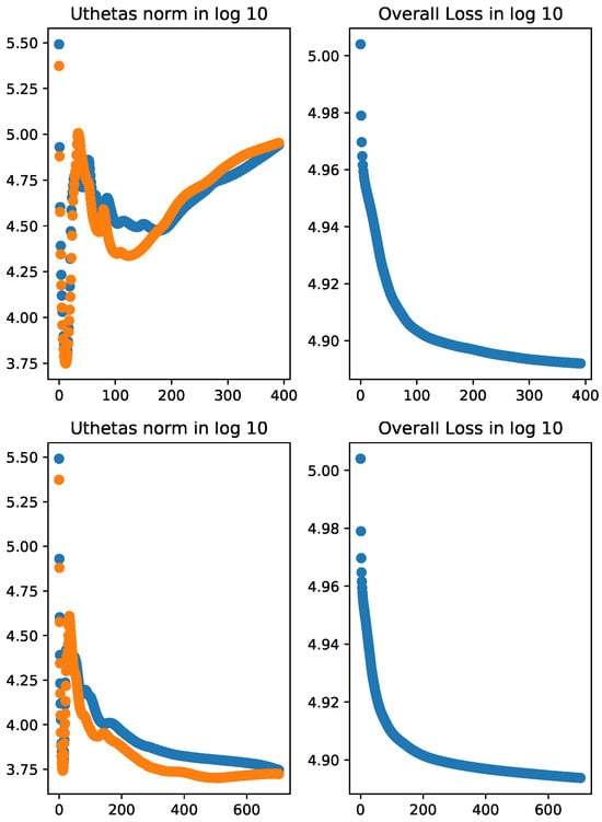
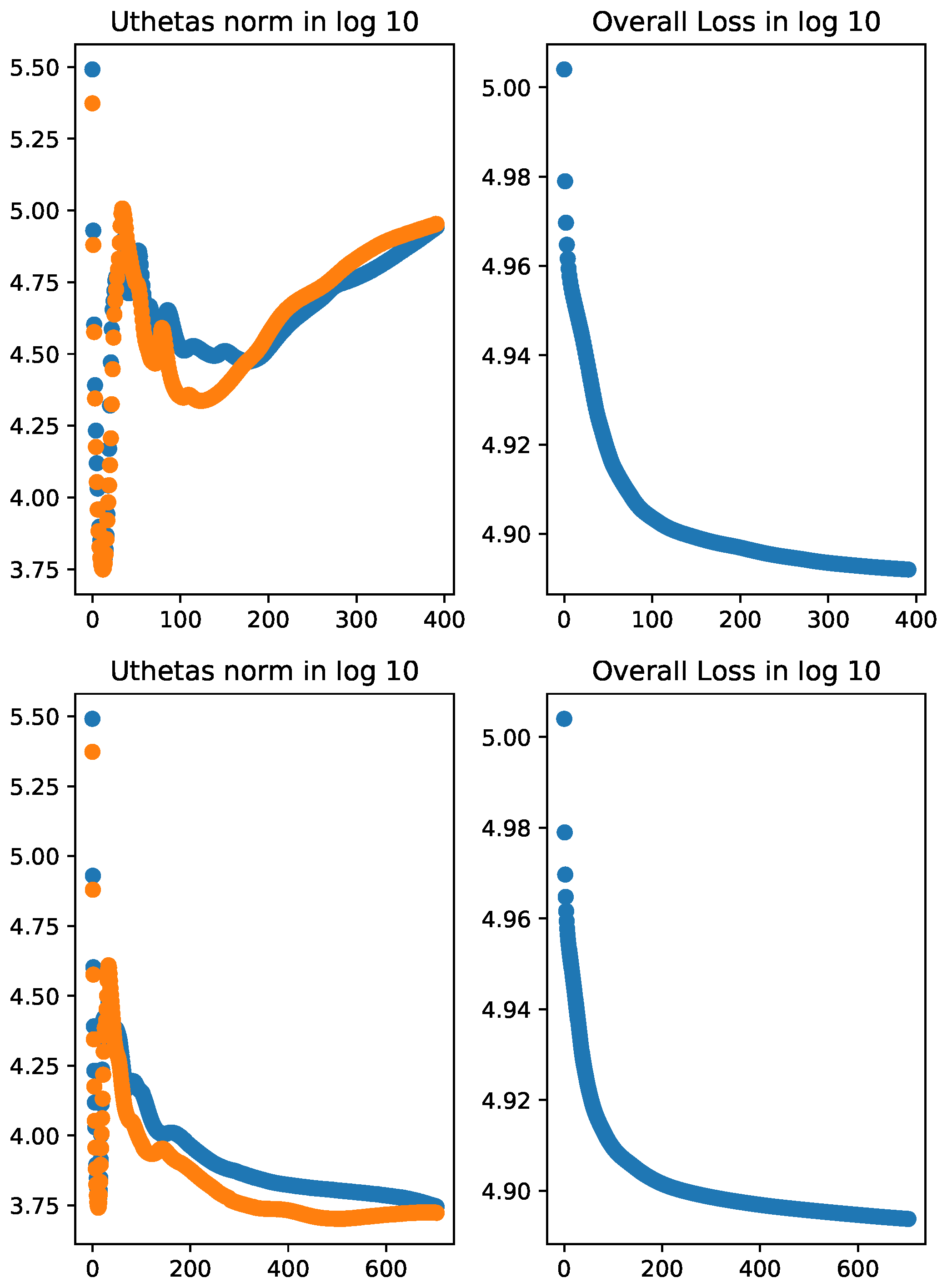
Figure 1.
norm of the score functions and (Uthetas norm) in blue and orange colors, respectively, and overall loss of the ZIG model in log10 scale. Top two panels: without learning rate adjustment; bottom two panels: with learning rate adjustment. All parameters were initialized with true parameter values except for . In the top panels, the norms of the score vectors decrease drastically in early iterations but increase over later iterations even though the overall loss is consistently reduced. In the bottom panels, the norms of the score vectors first show similar pattern as the top panel but consistently decrease in later iterations. The overall loss shows the desired reducing trend throughout all iterations.
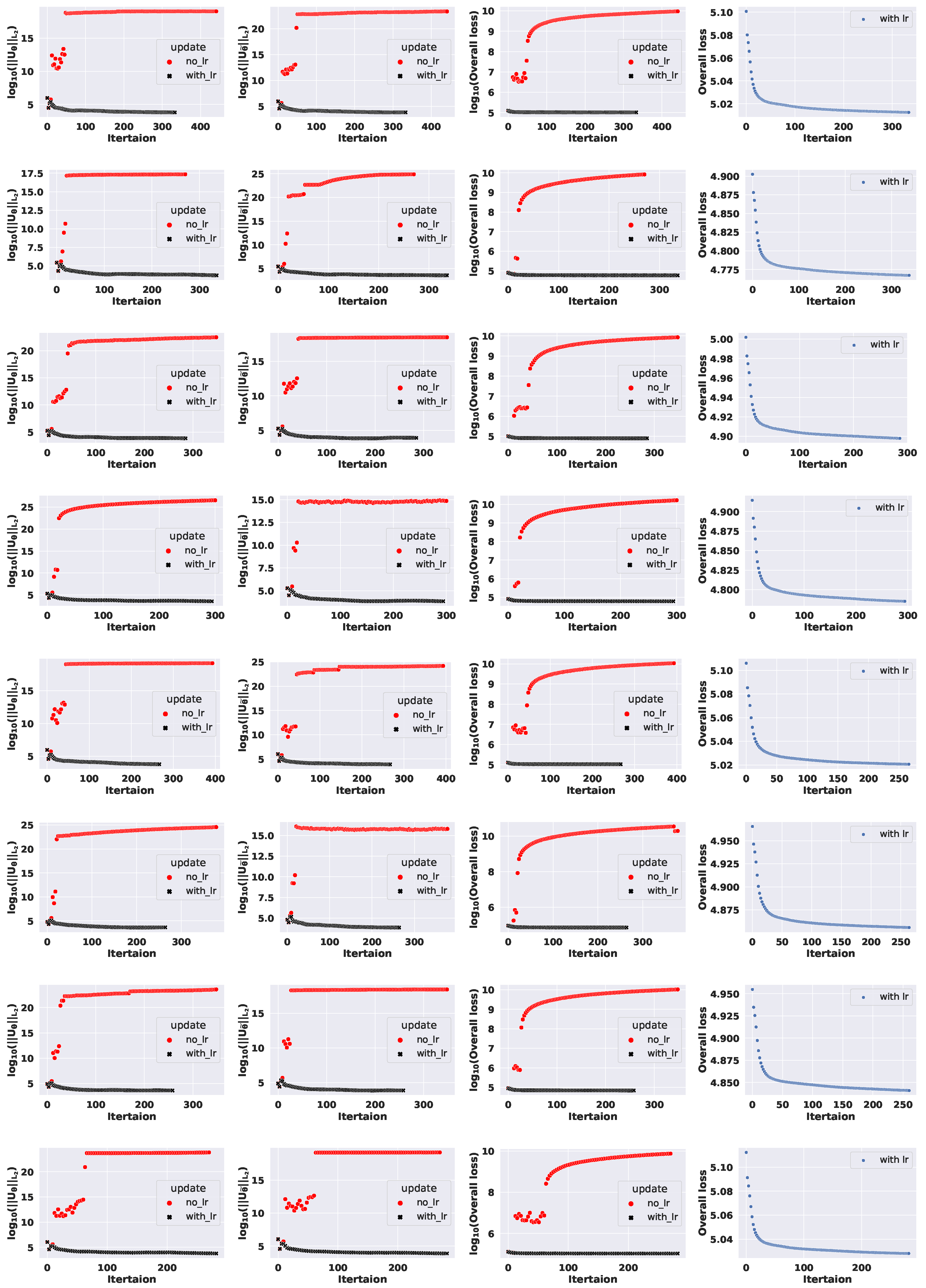
The results for Setting 2 are given in Figure 2. The last column shows the algorithm with learning rate adjustment alone because the scale of the third column is too high to see the reducing trend. In this case, with the initial values of all parameters generated randomly from Uniform distribution, the uncertainty in the parameters caused the algorithm without learning rate to breakdown. We see that the algorithm with no learning rate adjustment using updates in Algorithm 2 struggles to reduce the norms and headed toward wrong directions throughout the optimization process. On the other hand, the algorithm with learning rate adjustment had a little fluctuation at the beginning but continued toward the right direction by reducing both the norm of the score vectors and the loss function as the iterations proceed. Note that the dataset was identical for these two applications and both algorithms started with the same initial values. The only difference between the two algorithms is that learning rate adjustment is used in one algorithm but not in the other algorithm. Hence, the failure of the algorithm with no learning rate adjustment is due to the update being too big, which leads to the algorithm going toward wrong directions. The numerical study confirms that the alternating updates are capable of finding the maximum likelihood estimate, and learning rate adjustment in Algorithm 3 is an important component of the algorithm.
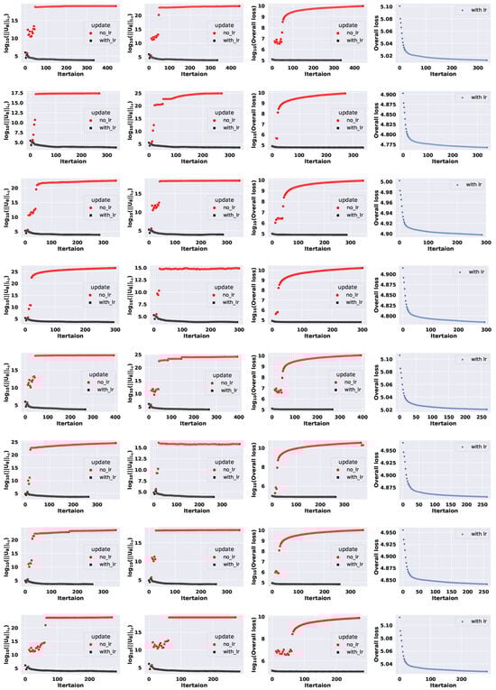
Figure 2.
Comparing performance of the alternating ZIG regression using log link with or without learning rate adjustment over 8 simulated datasets. Each row is for one dataset. First column: norm of ; second column: norm of ; third column: (overall loss); fourth column: overall loss of the algorithm with learning rate adjustment.
7.2. An Application of SA-ZIG on Word Embedding
In this section, we demonstrate the application of SA-ZIG using log link on a small dataset. This dataset comprises news articles sourced from the Reuters news archive. Using a Python script to simulate user clicks, we downloaded approximately 2000 articles from the Business category, spanning from 2019 to the summer of 2021. These articles are stored in an SQLite database. From this corpus, we created a small vocabulary consisting of the most frequently used words. We trained a -dimensional dense vector representation for each of the 300 words using the downloaded business news.
To apply the SA-ZIG model, we first obtain weighted word–word co-occurrence count, computed as follows:
where = separation between word i and word j in sentence s, and k is pre-determined window size 10.
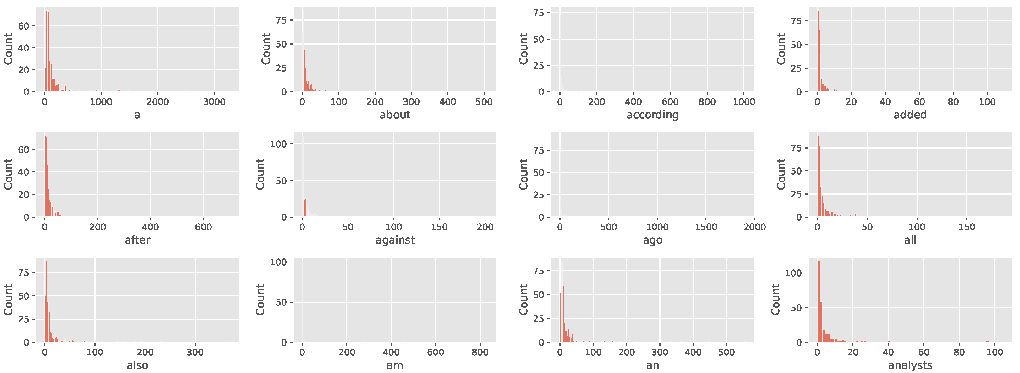
Figure 3 shows the histogram of the counts from the first 12 rows. The counts for each row are highly skewed and have a lot of zeros. It can be seen that zero-inflated Gamma may be suitable for the data.
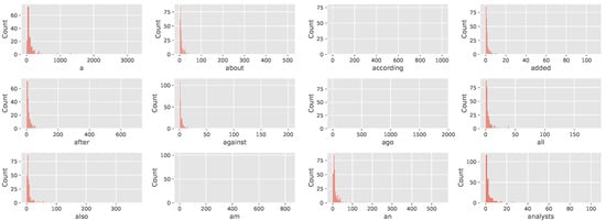
Figure 3.
Histogram of weighted count from each of the first 12 rows of the data matrix.
The co-occurrence matrix with sparse format was fed into the SA-ZIG model with learning rate adjustment. The parameters are initialized based on the following description:
- The entries in matrix were independently generated from uniform distribution between and with seed 99.
- The entries in matrix were generated from uniform distribution between and with seed 98.
- The V bias terms in were independently generated from uniform (−0.1, 0.1) with seed 97.
- The V bias terms in were independently generated from uniform (−0.1, 0.1) with seed 96.
- The V bias terms in were independently generated from uniform (0.1, 0.6) with seed 1.
- The bias terms in were independently generated from uniform (0.1, 0.6) with seed 2.
- The learning rate at iteration is set to as given in Algorithm 3 with .
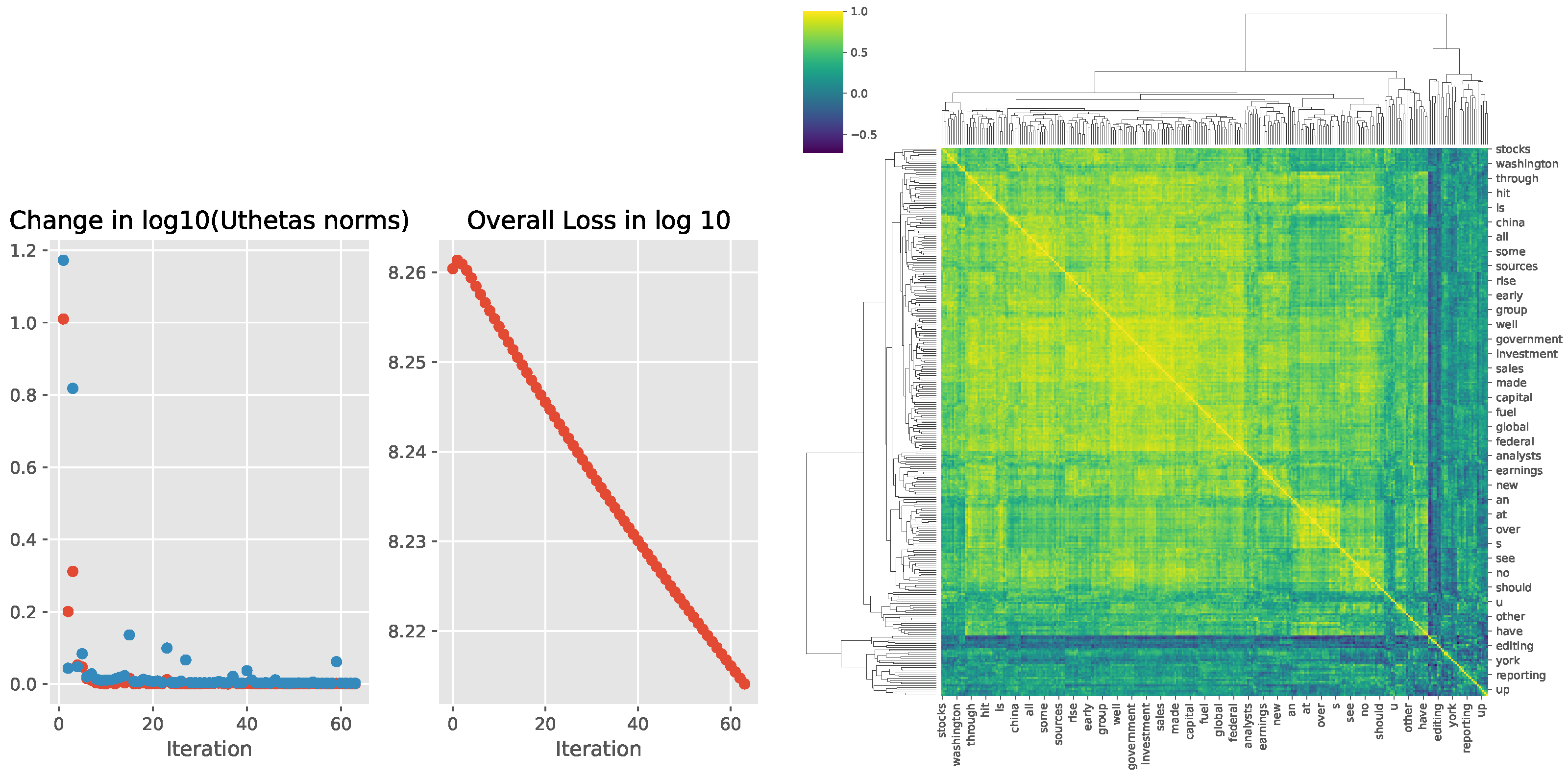
We let the model parameter update run 60 iterations in the outlier loop and 20 epochs in the inner loop. These numbers are used because the GloVe model training in [13] ran 50 iterations for vector dimensions ≤ 300. We want to see how the estimation proceeds with the iteration number. At the 60th iteration, the algorithm has not converged yet. This can be seen from the loss curve in Figure 4, which still sharply moves downward. The cosine similarity between word pairs is shown in the heatmap on the right panel of Figure 4.
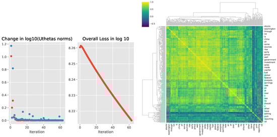
Figure 4.
(Left): The absolute value of change in the log10 norms of (red) and (blue) from successive iterations and overall loss curve. (Right): Cosine similarity of word vector representations shown as heatmap.
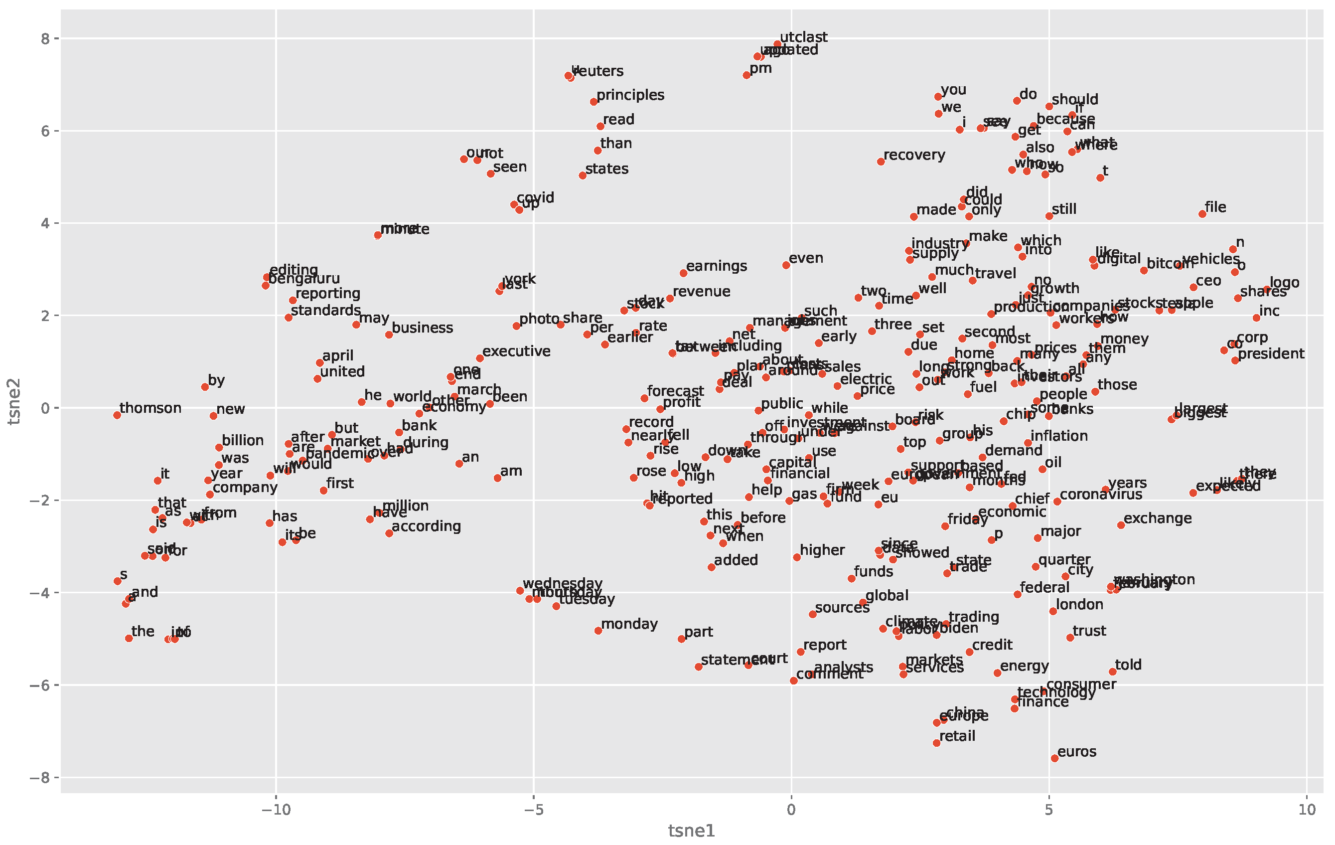
To visualize the relationships between different words, we first project the learned vector representations to the first 10 principal components (PCs). These 10 PCs cumulatively explained 97% of variations in the word vectors. We then conduct further dimension reduction with T-Distributed Stochastic Neighbor Embedding (t-SNE) to two-dimensional space. The t-SNE minimizes the divergence between two distributions: a distribution that measures pairwise similarities of the input objects and a distribution that measures pairwise similarities of the corresponding low-dimensional points in the embedding. The words on t-SNE coordinates are shown in Figure 5. Each point on the plot represents a word in the low-dimensional space. The closer two words are on the plot, the more similar they are in meaning or usage. For example, the top five most similar words to ‘capital’ from the 300 words are ‘firm’, ‘management’, ‘fund’, ‘board’, ‘financial’. These are based on the cosine similarity. The five most similar words to ‘stocks’ from the 300 words are ‘companies’, ‘bitcoin’, ‘banks’, ‘prices’ and ‘some’. The top five most similar words to ‘finance’ are ‘technology’, ‘energy’, ‘trading’, ‘consumer’, ‘analysts’. Words ‘monday’, ‘tuesday’, ‘wednesday’ are clustered together. This scatter plot captures some semantic similarities.
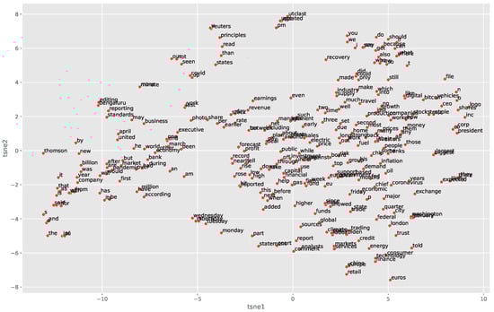
Figure 5.
Plot of word vector representations using t-SNE on first 10 principal components.
8. Conclusions and Discussion
In summary, we presented the shared parameter alternating zero-inflated Gamma (SA-ZIG) regression model in this paper. The SA-ZIG model is designed for highly skewed non-negative matrix data. It uses a logit link to model the zero versus positive observations. For the Gamma part, we considered two link functions: the canonical link and the log link, and derived updating formulas for both.
We proposed an algorithm that alternately updates the parameters and while holding one of them fixed. The Fisher scoring algorithm, with or without learning rate adjustment, was employed in each step of the alternating update. Numerical studies indicate that learning rate adjustment is crucial in SA-ZIG regression. Without it, the algorithm may fail to find the optimal direction.
After model estimation, the matrix is factorized into the product of a left matrix and a right matrix. The rows of the left matrix and the columns of the right matrix provide vector representations for the rows and columns, respectively. These estimated row and column vector representations can then be used to assess the relevance of items and make recommendations in downstream analysis.
The SA-ZIG model is inherently similar to factor analysis. In factor analysis, both the loading matrix and the coefficient vector are unknown. The key difference between SA-ZIG and factor analysis is that SA-ZIG uses a large coefficient matrix, whereas factor analysis uses a single vector. Additionally, SA-ZIG assumes a two-stage Bernoulli–Gamma model, while factor analysis assumes a normal distribution.
In both models, likelihood-based estimation can determine convergence behavior by linking the complete data likelihood with the conditional likelihood. For factor analysis, the normal distribution and the linearity of the sufficient statistic in the observed data allow the use of ALS to estimate both the loading matrix and the coefficient vector ([31]). However, SA-ZIG cannot use ALS because the variance of the Gamma distribution is not constant.
In both SA-ZIG and factor analysis, the unobserved row (or column) vector representation and the factor loading matrix can be treated as missing data, assuming the data are missing completely at random. For missing data analysis, the well-known Expectation Maximization (EM) algorithm can be used to estimate parameters. The EM algorithm has the advantageous property that successive updates always move towards maximizing the log likelihood. It works well when the proportion of missing data is small, but it is notoriously slow when a large amount of data is missing.
For SA-ZIG, the alternating scheme with the Fisher scoring algorithm offers the benefit of a quadratic rate of convergence if the true parameters and their estimates lie within the interior of the parameter space. However, in real applications, the estimation process might diverge at either stage of the alternating scheme because the Fisher scoring update does not always guarantee an upward direction, especially in cases of complete or quasi complete separation. Additionally, the algorithm may struggle to find the optimal solution due to the non-identifiability of the row and column matrices under orthogonal transformations, leading to a ridge of solutions. The learning rate adjustment in Algorithm 3 helps by making small moves during successive updates in later stage of the algorithm and thereby is more likely to find a solution.
Future research on similar problems could explore alternative distributions beyond Gamma. Tweedie and Weibull distributions, for instance, are capable of modeling both symmetric and skewed data through varying parameters, each with its own associated link functions. However, new algorithms and convergence analyses would need to be developed specifically for these distributions. In practical applications, the most suitable distribution for the observed data is often uncertain, making diagnostic procedures an important area for further investigation.
Author Contributions
Methodology, T.K. and H.W.; Software, T.K. and H.W.; Validation, T.K.; Writing—original draft, T.K. and H.W.; Writing—review & editing, T.K. and H.W.; Supervision, H.W. All authors have read and agreed to the published version of the manuscript.
Funding
This research received no external funding.
Data Availability Statement
The original contributions presented in the study are included in the article, further inquiries can be directed to the corresponding author.
Conflicts of Interest
The authors declare no conflicts of interest.
References
- Edelman, A.; Jeong, S. Fifty three matrix factorizations: A systematic approach. arXiv 2022, arXiv:2104.08669. [Google Scholar] [CrossRef]
- Gan, J.; Liu, T.; Li, L.; Zhang, J. Non-negative Matrix Factorization: A Survey. Comput. J. 2021, 64, 1080–1092. [Google Scholar] [CrossRef]
- Saberi-Movahed, F.; Berahman, K.; Sheikhpour, R.; Li, Y.; Pan, S. Nonnegative matrix factorization in dimensionality reduction: A survey. arXiv 2024, arXiv:2405.03615. [Google Scholar]
- Wang, Y.-X.; Zhang, Y.-J. Nonnegative matrix factorization: A comprehensive review. IEEE Trans. Knowl. Data Eng. 2013, 25, 1336–1353. [Google Scholar] [CrossRef]
- Koren, Y. Factorization meets the neighborhood: A multifaceted collaborative filtering model. In Proceedings of the 14th ACM SIGKDD International Conference on Knowledge Discovery and Data Mining, KDD ’08, Las Vegas, NV, USA, 24–27 August 2008; Association for Computing Machinery: New York, NY, USA, 2008; pp. 426–434. [Google Scholar]
- Zhang, Z.; Liu, H. Social recommendation model combining trust propagation and sequential behaviors. Appl. Intell. 2015, 43, 695–706. [Google Scholar] [CrossRef]
- Fernández-Tobías, I.; Cantador, I.; Tomeo, P.; Anelli, V.W.; Di Noia, T. Addressing the user cold start with cross-domain collaborative filtering: Exploiting item metadata in matrix factorization. User Model. User-Adapt. Interact. 2019, 29, 443–486. [Google Scholar] [CrossRef]
- Puthiya Parambath, S.A.; Chawla, S. Simple and effective neural-free soft-cluster embeddings for item cold-start recommendations. Data Min. Knowl. Discov. 2020, 34, 1560–1588. [Google Scholar] [CrossRef]
- Nguyen, P.; Wang, J.; Kalousis, A. Factorizing lambdaMART for cold start recommendations. Mach. Learn. 2016, 104, 223–242. [Google Scholar] [CrossRef]
- Panda, D.K.; Ray, S. Approaches and algorithms to mitigate cold start problems in recommender systems: A systematic literature review. J. Intell. Inf. Syst. 2022, 59, 341–366. [Google Scholar] [CrossRef]
- Mikolov, T.; Chen, K.; Corrado, G.S.; Dean, J. Efficient estimation of word representations in vector space. arXiv 2013, arXiv:1301.3781. [Google Scholar]
- Mikolov, T.; Sutskever, I.; Chen, K.; Corrado, G.S.; Dean, J. Distributed representations of words and phrases and their compositionality. In Advances in Neural Information Processing Systems; Burges, C., Bottou, L., Welling, M., Ghahramani, Z., Weinberger, K., Eds.; Curran Associates, Inc.: Red Hook, NY, USA, 2013; Volume 26. [Google Scholar]
- Pennington, J.; Socher, R.; Manning, C.D. Glove: Global vectors for word representation. In Proceedings of the 2014 Conference on Empirical Methods in Natural Language Processing (EMNLP), Doha, Qatar, 25–29 October 2014; pp. 1532–1543. [Google Scholar]
- Mills, E.D. Adjusting for Covariates in Zero-Inflated Gamma and Zero-Inflated Log-Normal Models for Semicontinuous Data. Ph.D. Dissertation, University of Iowa, Iowa City, IA, USA, 2013. [Google Scholar] [CrossRef]
- Wei, X.-X.; Zhou, D.; Grosmark, A.D.; Ajabi, Z.; Sparks, F.T.; Zhou, P.; Brandon, M.P.; Losonczy, A.; Paninski, L. A zero-inflated gamma model for post-deconvolved calcium imaging traces. Neural Data Sci. Anal. 2020, 3. [Google Scholar] [CrossRef]
- Nobre, A.A.; Carvalho, M.S.; Griep, R.H.; Fonseca, M.d.J.M.d.; Melo, E.C.P.; Santos, I.d.S.; Chor, D. Multinomial model and zero-inflated gamma model to study time spent on leisure time physical activity: An example of elsa-brasil. Rev. Saúde Pública 2017, 51, 76. [Google Scholar] [CrossRef] [PubMed]
- Moulton, L.H.; Curriero, F.C.; Barroso, P.F. Mixture models for quantitative hiv rna data. Stat. Methods Med. Res. 2002, 11, 317–325. [Google Scholar] [CrossRef] [PubMed]
- Wu, M.C.; Carroll, R.J. Estimation and comparison of changes in the presence of informative right censoring by modeling the censoring process. Biometrics 1988, 44, 175–188. [Google Scholar] [CrossRef]
- Have, T.R.T.; Kunselman, A.R.; Pulkstenis, E.P.; Landis, J.R. Mixed effects logistic regression models for longitudinal binary response data with informative drop-out. Biometrics 1998, 54, 367–383. [Google Scholar] [CrossRef]
- Albert, P.S.; Follmann, D.A.; Barnhart, H.X. A generalized estimating equation approach for modeling random length binary vector data. Biometrics 1997, 53, 1116–1124. [Google Scholar] [CrossRef]
- Du, J. Which Estimator of the Dispersion Parameter for the Gamma Family Generalized Linear Models Is to Be Chosen? Master’s Thesis, Dalarna University, Falun, Sweden, 2007. Available online: https://api.semanticscholar.org/CorpusID:34602767 (accessed on 23 October 2024).
- Haberman, S. The Analysis of Frequency Data; Midway reprint; University of Chicago Press: Chicago, IL, USA, 1977. [Google Scholar]
- Silvapulle, M.J. On the existence of maximum likelihood estimators for the binomial response models. J. R. Stat. Soc. Ser. B-Methodol. 1981, 43, 310–313. [Google Scholar] [CrossRef]
- Albert, A.; Anderson, J.A. On the existence of maximum likelihood estimates in logistic regression models. Biometrika 1984, 71, 1–10. [Google Scholar] [CrossRef]
- Marschner, I.C. glm2: Fitting generalized linear models with convergence problems. R J. 2011, 3, 12–15. [Google Scholar] [CrossRef]
- Boyd, S.; Vandenberghe, L. Convex Optimization; Cambridge University Press: Cambridge, UK, 2004. [Google Scholar]
- Givens, G.H.; Hoeting, J.A. Computational Statistics, 2nd ed.; John Wiley & Sons, Inc.: Hoboken, NJ, USA, 2013. [Google Scholar]
- Osborne, M.R. Fisher’s method of scoring. Int. Stat. Rev. Rev. Int. Stat. 1992, 60, 99–117. [Google Scholar] [CrossRef]
- Reddi, S.J.; Kale, S.; Kumar, S. On the convergence of adam and beyond. In Proceedings of the International Conference on Learning Representations, Vancouver, BC, Canada, 30 April–3 May 2018. [Google Scholar]
- Shi, N.; Li, D.; Hong, M.; Sun, R. RMSprop converges with proper hyper-parameter. In Proceedings of the 9th International Conference on Learning Representations (ICLR 2021), Online, 3–7 May 2021. [Google Scholar]
- Dempster, A.P.; Laird, N.M.; Rubin, D.B. Maximum likelihood from incomplete data via the em algorithm. J. R. Stat. Soc. Ser. B (Methodol.) 1977, 39, 1–22. [Google Scholar] [CrossRef]
Disclaimer/Publisher’s Note: The statements, opinions and data contained in all publications are solely those of the individual author(s) and contributor(s) and not of MDPI and/or the editor(s). MDPI and/or the editor(s) disclaim responsibility for any injury to people or property resulting from any ideas, methods, instructions or products referred to in the content. |
© 2024 by the authors. Licensee MDPI, Basel, Switzerland. This article is an open access article distributed under the terms and conditions of the Creative Commons Attribution (CC BY) license (https://creativecommons.org/licenses/by/4.0/).