Efficient Structural Damage Detection with Minimal Input Data: Leveraging Fewer Sensors and Addressing Model Uncertainties

Abstract

In the field of structural damage detection through vibration measurements, most existing methods demand extensive data collection, including vibration readings at multiple levels, strain data, temperature measurements, and numerous vibration modes. These requirements result in high costs and complex instrumentation processes. Additionally, many approaches fail to account for model uncertainties, leading to significant discrepancies between the actual structure and its numerical reference model, thus compromising the accuracy of damage identification. This study introduces an innovative computational method aimed at minimizing data requirements, reducing instrumentation costs, and functioning with fewer vibration modes. By utilizing information from a single vibration sensor and at least three vibration modes, the method avoids the need for higher-mode excitation, which typically demands specialized equipment. The approach also incorporates model uncertainties related to geometry and mass distribution, improving the accuracy of damage detection. The computational method was validated on a steel frame structure under various damage conditions, categorized as single or multiple damage. The results indicate up to 100% accuracy in locating damage and up to 80% accuracy in estimating its severity. These findings demonstrate the method’s potential for detecting structural damage with limited data and at a significantly lower cost compared to conventional techniques.

1. Introduction

Structural damage detection has garnered significant attention over the past few decades due to its importance in ensuring the safety and longevity of civil infrastructures. Damage detection methodologies can generally be categorized into local and global methods. While local methods offer high precision in identifying damage location, they often require predefined search regions and unrestricted access to structural components, which is not always feasible. On the other hand, global methods, particularly those relying on vibration response measurements, have proven more practical for large structures where accessibility and instrumentation are limited. These vibration-based methods utilize either raw signals, such as acceleration and velocity, or processed data like modal frequencies and shapes to detect damage, offering a non-destructive means of structural health monitoring [1,2,3,4,5,6,7,8,9,10,11,12,13]. Despite their benefits, these methods face challenges related to the complexity and non-linear behavior of structures [14]. Recent developments in the use of neural networks for predicting structural behaviors have demonstrated a strong ability to handle large datasets and adapt to the physical conditions of the environment. In particular, it has been shown that a physics-informed neural network can predict stratified ground consolidation using minimal pore water pressure data over a short period [15]. These advances underscore the importance of approaches that minimize data requirements without compromising precision.

Global vibration-based damage detection methods have been extensively studied since the 1970s and are particularly valuable for detecting early-stage damage in civil structures [16,17,18,19], which is crucial for preventing catastrophic failures and reducing economic losses. However, the effectiveness of these methods is often limited by several practical constraints. Among these are the high costs associated with instrumentation, as current methodologies require substantial input data, such as vibration histories from various measurement points and a large number of mode shapes. This necessitates a finer measurement grid, which translates to a greater number of sensors [20]. Additionally, there are challenges in exciting higher-order modal frequencies and experimentally capturing all degrees of freedom (DOFs).

Acquiring high-frequency mode shapes in buildings presents multiple technical and practical challenges. First, exciting high-frequency modes requires significantly more energy, making conventional methods, such as impact hammers or shakers, less effective. In ambient vibration tests, higher modes are rarely excited efficiently [21]. Furthermore, structural damping increases with frequency, attenuating higher modes more rapidly, especially in materials like concrete, making them harder to detect. Additionally, data acquisition systems must operate at very high sampling rates to capture high-frequency vibrations, significantly increasing computational demands. Specialized equipment, such as high-frequency shakers, is expensive and challenging to install, and higher numbers of mode shapes are generally more difficult to interpret, requiring a higher density of sensors. Limited access to measurement points, particularly in large buildings, further complicates the process, as installing sensors in hard-to-reach areas can be difficult.

Another critical challenge for existing damage detection methods lies in the discrepancies between experimental and numerical models. A limited number of measured DOFs often necessitate finite element (FE) model reduction or experimental data expansion, which can introduce interpolation or truncation errors, ultimately affecting the accuracy of damage detection [2,3,4,21,22,23,24].

Uncertainties are inherent in both structural models and measurements, posing a significant limitation to damage detection methods, which often fail to account for these factors. Astroza [25] incorporates model uncertainties, such as geometry, mass distribution, and nodal loads, into the model updating process. The author stresses that neglecting these uncertainties can result in poor damage detection accuracy, and thus recommends their inclusion in damage detection methodologies.

Measurement noise, environmental conditions, and modeling errors—such as uncertainty in material properties or geometric simplifications—substantially impact the accuracy of FE models, potentially leading to false positives or incorrect identification of damage [20,25,26,27,28]. To mitigate these issues, optimization techniques, particularly genetic algorithms (GAs), have been increasingly applied. These algorithms, inspired by natural evolutionary processes, offer robust solutions to the inverse problem in damage detection by optimizing objective functions sensitive to changes in structural parameters [29,30,31].

In this study, we propose a low-cost computational methodology for structural damage detection that utilizes genetic algorithms while incorporating geometric uncertainties to improve detection accuracy. This approach is designed to function effectively with limited and incomplete modal data, addressing two major challenges in current damage detection techniques: the scarcity of modal frequencies and mode shapes obtainable from large civil structures, and the limitations imposed by the high costs of sensor deployment. Unlike traditional methods that require numerous frequencies and mode shapes for reliable damage detection, the proposed computational method performs well with minimal data, thereby reducing instrumentation costs and minimizing the risk of structural damage due to high-frequency excitation. Furthermore, this methodology circumvents the need for FE model reduction or data expansion, eliminating the associated errors and enhancing the accuracy of damage identification.

The remainder of this manuscript is organized as follows: Section 2 addresses the issue of geometric uncertainties and presents how these are handled in the proposed methodology. Section 3 discusses the limitations of experimental modal data and the necessity of accommodating these constraints in damage detection. Section 4 introduces the problem of incomplete data, and the solution provided by this computational methodology. In Section 5, the development and implementation of the genetic algorithm are detailed, followed by results and conclusions in Section 6 and Section 7, respectively.

2. Uncertainty Considerations

In vibration-based damage identification methods with model data, it is common to compare two models: the model representing the undamaged state, typically a finite element model, and the model representing the damaged state, mostly an experimental model. Discrepancies between a real model and its finite element representation are well documented, arising from modeling errors or simplifications. To address this challenge, various solutions, including model updating [25,32,33,34,35,36,37,38,39,40,41,42,43,44] have been proposed. The objective of these solutions is to minimize the disparities between the actual model and its finite element counterpart. This method serves as the cornerstone for model-based damage detection approaches.

Model updating in finite element modeling is defined as the process of refining an FE model to minimize discrepancies between measured responses and those predicted by the model. This inverse problem entails determining a set of model parameters to minimize an objective function, quantifying the disparity between actual responses and those predicted by the FE model. Model updating in the FE domain stands out as an effective and conventional methodology for damage identification purposes, providing valuable insights into the existence and location of damage. However, a drawback associated with the model updating method is the requirement for pre- and post-damage vibration data to obtain an accurate approximation of the real model. Unfortunately, obtaining pre-damage information is often challenging and unavailable in many real-world scenarios [25]. Furthermore, the computational methodology for damage identification based on model updating involves two primary sources of uncertainty: measurement noise and modeling errors. Diverse approaches have been proposed to mitigate the effects of measurement noise, and these have been extensively studied [45]. Regarding modeling errors, which encompass both parameter and model uncertainties, they constitute the primary source of uncertainty in damage identification.

The finite element method (FEM) is a widely used computational technique in structural engineering that allows engineers to analyze and predict the behavior of complex structures under various conditions. This method divides a structure into smaller, simpler components called “elements”, which are connected at points known as “nodes”. By modeling each element and its interactions with others, engineers can simulate how the entire structure will respond to external forces, such as vibrations, loads, and environmental conditions.

In the context of damage detection, it is essential to understand how structures behave dynamically—that is, how they respond to forces that change over time, such as earthquakes, wind, or impacts. The dynamic equations of motion (represented as Equation (1)) describe this behavior by incorporating three fundamental properties of the structure: mass, stiffness, and damping. Mass refers to the amount of material in the structure, which affects how much force is needed to cause it to accelerate or deform. Stiffness is a measure of how much a structure resists deformation when a force is applied. A stiffer structure will deform less under the same load compared to a less stiff structure. Damping represents the ability of a structure to dissipate energy, which helps to reduce vibrations and oscillations over time. Structures with higher damping can absorb and dissipate energy more effectively, reducing the risk of damage during dynamic events.

Equation (1) combines these properties to provide a mathematical representation of how the structure moves and behaves when subjected to dynamic forces.

Furthermore, to effectively detect damage within a structure, engineers must also consider the modal problem, described by Equation (2). This aspect focuses on the natural frequencies and mode shapes of the system. Natural frequencies are the specific frequencies at which a structure tends to vibrate when disturbed. Each structure has its own unique set of natural frequencies based on its physical properties. Mode shapes describe the pattern of displacement that the structure undergoes at each natural frequency. They indicate how different parts of the structure move in relation to one another when it vibrates.

By analyzing the natural frequencies and mode shapes, engineers can identify changes or anomalies that may indicate structural damage. Such changes can manifest as shifts in natural frequencies or alterations in mode shapes, which can be critical for ensuring the safety and integrity of the structure.

In summary, the finite element method provides a powerful framework for modeling the dynamic behavior of structures, while the dynamic equations of motion and the modal problem are essential tools for detecting and diagnosing damage in those structures.

Astroza et al. [25,33] thoroughly investigated the effects of model parameter uncertainties in updating methods, proposed that considering these uncertainties is crucial for achieving accurate damage identification, and incorporated a vector of parameters associated with model uncertainties, denoted as φ, and another vector of parameters to be estimated, denoted as θ, into the structural model (Equation (1)). In other words, θ represents the values with which the model will be updated. The vector of parameters associated with model uncertainties includes parameters such as geometry, masses, gravitational loads, and damping properties, representing conditions of model uncertainty that are inherently present. This is because the finite element model is never a perfect representation of the structure being modeled.

$$\mathbf{M}\left(\mathit{\theta },\mathit{\phi }\right)\ddot{\mathit{q}}+\mathbf{C}\left(\mathit{\theta },\mathit{\phi }\right)\dot{\mathit{q}}+\mathit{r}\left(\mathit{q},\mathit{\theta },\mathit{\phi }\right)=-\mathbf{M}\left(\mathit{\theta },\mathit{\phi }\right)\mathit{L}\left(\mathit{\theta },\mathit{\phi }\right)\ddot{\mathit{u}}$$

(1)

where M and C are the mass and damping matrices, respectively. $\mathit{q},\dot{\mathit{q}},\ddot{\mathit{q}}$ represent the displacement vector, velocity, and nodal acceleration, respectively; $\mathit{r}\left(\mathit{q},\mathit{\theta },\mathit{\phi }\right)$ is the internal resistance force, $\mathit{L}\left(\mathit{\theta },\mathit{\phi }\right)$ is the excitation influence matrix from the base, and $\ddot{\mathit{u}}$ is the input ground acceleration. The uncertainties considered in a structural model depend on the type of analysis conducted and involve only the relevant parameters. In the methodology for damage detection using modal data, only parameters related to modal analysis are involved to avoid unnecessary unknowns. The structural model for modal analysis employed in this study, as depicted in Equation (2), has been utilized in prior works [2,46], and assumes linear behavior both before and after damage occurrence—this assumption has been used by several authors in their damage detection computation methodologies [11,47,48,49,50,51].

$$\left[\mathbf{K}-{\lambda }_i\mathbf{M}\right]\left\{{\mathit{\varphi }}_{\mathit{i}}\right\}=\left\{0\right\}$$

(2)

To address the uncertainties within the system and incorporate them into the model to mitigate their effects on damage detection, the vector of parameters associated with system uncertainty is defined as follows:

$$\mathit{\phi }=[\mathbf{H},\mathbf{V},\overline{\mathit{m}}]$$

(3)

where H, V, and $\overline{\mathit{m}}$ are the horizontal and vertical coordinates and distributed masses, respectively. This vector contains information about system uncertainties related to geometry and distributed masses. Equation (2) is expressed in terms of the uncertainty vector as defined below:

$$\left[\mathbf{K}\left(\mathit{\phi }\right)-{\lambda }_i\mathbf{M}\left(\mathit{\phi }\right)\right]\left\{{\mathit{\varphi }}_{\mathit{i}}\right\}=\left\{0\right\}$$

(4)

$${\lambda }_i={\omega }_i^2$$

(5)

The previous model is expressed in terms of the uncertainty parameters of the system related to the type of analysis and will be employed in the damage detection algorithm. The percentage of uncertainty in the specified parameters is constrained according to Astroza’s work [25], wherein an error in magnitude range of 3 to 10% is defined for horizontal and vertical coordinates, and for masses, a range of 5 to 30% is established.

3. Limitation of Modal Data

In general, modal tests conducted using specialized software generate a substantial amount of data, with limitations primarily dictated by computational capabilities. Conversely, laboratory tests can also yield significant data; however, they begin to encounter limitations as well. For instance, while the number of measurement points (sensors) can be extensive, this is often contingent upon the cost and precision of the sensors employed. Although laboratory tests may utilize numerous sensors, this number is significantly lower compared to what a finite element model might encompass.

Moreover, the excitation mechanisms for laboratory structures are typically more economical and easier to implement. In contrast, the modal data obtained from experimental tests on real structures is often limited. The primary constraints arise from the necessity of measurement points, as the sensors used in such tests can be prohibitively expensive. For example, high-quality accelerometers required for accurate modal testing can cost thousands of dollars each, which restricts the number of sensors that can be deployed. Furthermore, the two most common excitation techniques—namely, impact hammers and shakers—also incur considerable costs when applied to real structures. This expense is compounded by the practical difficulties associated with exciting higher-order modal frequencies in large-scale structures.

A comprehensive review of operational modal analysis on bridges outlines the challenges specific to real-world applications. It highlights the need for sufficient sensor density and strategic placement to accurately capture dynamic behavior, which can be impeded by both financial constraints and access difficulties in large structures [52,53]. Typically, existing modal testing techniques can achieve a low-frequency range, thereby restricting the number of modal shapes that can be obtained.

Special care must be exercised when employing these techniques; incorrect usage can lead to structural damage. For large structures, ambient vibration testing (AVT) is often utilized due to the challenges involved in exciting them using dynamic actuators or impact hammers. While AVT is advantageous in its non-intrusiveness, it is primarily suitable for modal tests focused on lower modes [54]. Additionally, environmental conditions, such as background noise or vibrations from nearby activities, can interfere with accurate measurements. In one case study [55], researchers conducting modal analysis on a large bridge encountered significant noise from vehicular traffic, which obscured the modal data. This necessitated the implementation of advanced filtering techniques to isolate the relevant signals, thereby complicating the data acquisition process.

Many damage identification techniques assume that the modal information of the studied structure is comprehensive and devoid of limitations [1,21,56]. This assumption arises because the methodologies are often developed based on laboratory specimens and do not account for the constraints faced in real-world applications. In essence, the accuracy of damage identification is heavily reliant on a high number of input frequencies and modal shapes.

In the proposed computational methodology, the authors address these limitations by utilizing a restricted number of frequencies and modal shapes. Notably, the method operates effectively with a minimum of three identified modal shapes and natural frequencies derived from the experimental model. It is important to highlight that the approach is restricted to longitudinal modes and does not include torsional modes. Despite these limitations, the damage identification method has demonstrated promising results in preliminary tests, indicating its potential applicability even within constrained conditions.

4. Incomplete Data Problem

In damage identification methodologies based on models, the comparison of two models is essential, and an objective function representing the differences between these models is minimized. To enable a meaningful comparison, an equal number of measurement points is required on both ends. However, it is acknowledged that the information available in the experimental model is invariably less than that in the finite element (FE) model. This discrepancy arises from the impracticality of placing a sensor for each degree of freedom (DOF) in the FE model due to the associated cost constraints and logistical difficulties. Moreover, the measurement of rotational degrees of freedom proves intricate. Consequently, the implementation of either FE model reduction techniques or an expansion of experimental data becomes crucial [30,57,58]. However, the incorporation of these techniques introduces truncation errors in the model reduction or interpolation errors in the data expansion [22]. These errors significantly impact the precision of damage identification, leading to the emergence of false positives or, in some cases, a failure to identify the correct element.

The proposed solution in this work for the previously stated problem involves a one-to-one comparison of the measured degrees of freedom (DOFs) with the DOFs of the FE model, without the need for model reduction or data expansion. This approach is justified by the fact that a one-to-one comparison of the DOFs in each model minimizes truncation and interpolation errors. It ensures that the comparison is conducted with precise and reliable data, as the measured DOFs accurately represent the real system response, making them more relevant for damage detection. The one-to-one comparison of DOFs is a straightforward method that does not necessitate expensive computational techniques. It allows for a direct validation with the experimental data, thereby enhancing confidence in the damage detection results. Additionally, the results obtained through the one-to-one comparison of the measured DOFs are compared with those obtained by implementing reduction and expansion techniques, demonstrating superior outcomes with the proposed solution. Equation (6) can be solved using various methods to obtain the vector of eigenvalues and eigenvectors.

$$\left[\mathsf{\Phi },\mathsf{\Lambda }\right]=eig\left(\mathbf{K},\mathbf{M}\right)$$

(6)

where $\mathsf{\Phi }$ is the matrix containing the modal vectors $\mathit{\varphi }$ and $\mathsf{\Lambda }$ is the matrix of squared circular frequencies ${\omega }^2$; $\mathbf{K}$ and $\mathbf{M}$ are the stiffness and mass matrices, respectively. The FE model contains N degrees of freedom, while the experimental model involves $N_s$ measurement points. The difference between both models is defined as shown in Equation (7), with the comparison performed exclusively at the experimental measurement points.

$$\Delta \epsilon =\sum _{j=1}^{N_m} {\left|{\mathit{\lambda }}_j^a-{\mathit{\lambda }}_j^x\right|}^2+\sum _{j=1}^{N_m}\sum _{i=1 }^{N_s}{ \left|{\mathit{\varphi }\left(i\right)}_j^a-{\mathit{\varphi }\left(i\right)}_j^x\right|}^2$$

(7)

where N_s is the number of measurement points in the experimental model, N_m is the number of experimentally identified modes, “$a$” refers to the finite element model, and “$x$” refers to the experimental model. This technique avoids errors introduced by reduction and expansion methods. Additionally, the damage identification methodology has demonstrated its effective handling of incomplete data and increased efficiency when implemented with the proposed technique.

5. Damage Detection Algorithm

Evolutionary optimization algorithms, such as genetic algorithms (GAs), play a significant role in damage identification methodologies [1,7,8,21,22,30,59,60,61,62,63]. Grounded in heuristic principles, such as natural selection and genetic operations, these algorithms are categorized into four groups: evolutionary programming (EP), evolutionary strategies (ESs), genetic programming (GP), and genetic algorithms (GAs). This investigation specifically concentrates on utilizing GAs for the identification of damage in structures through the optimization of an error function. The computational methodology involves the generation of a population comprising potential individual solutions, typically chosen at random. Each individual undergoes fitness evaluation, succeeded by the generation of a new population through recombination, crossover, and mutation processes, aiming to augment the most prominent fitness. The algorithm advances through successive generations to attain an optimal solution for damage identification [22].

One of the initial steps in the methodology is the encoding of the individual, which is of great importance in problem solving. In this work, the individual is composed of all the finite elements that make up the structure; each of these finite elements is represented by a chromosome, and in turn, these chromosomes are composed of genes that represent the physical properties (length, Young’s modulus, density, etc.) of the finite elements. An illustrative example of the encoded individual (χ) is presented in

Table 1. Example of encoded individual (χ), chromosomes and genes.

Chromosome	Gen 1	Gen 2	Gen 3	Gen 4	Gen 5
1	Length 1	Modulus 1	Density 1	Cross section 1	Angle 1
N	Length n	Modulus n	Density n	Cross section n	Angle n

. Where it is composed of five genes (but not limited to five, it can be n genes) and “n” chromosomes.

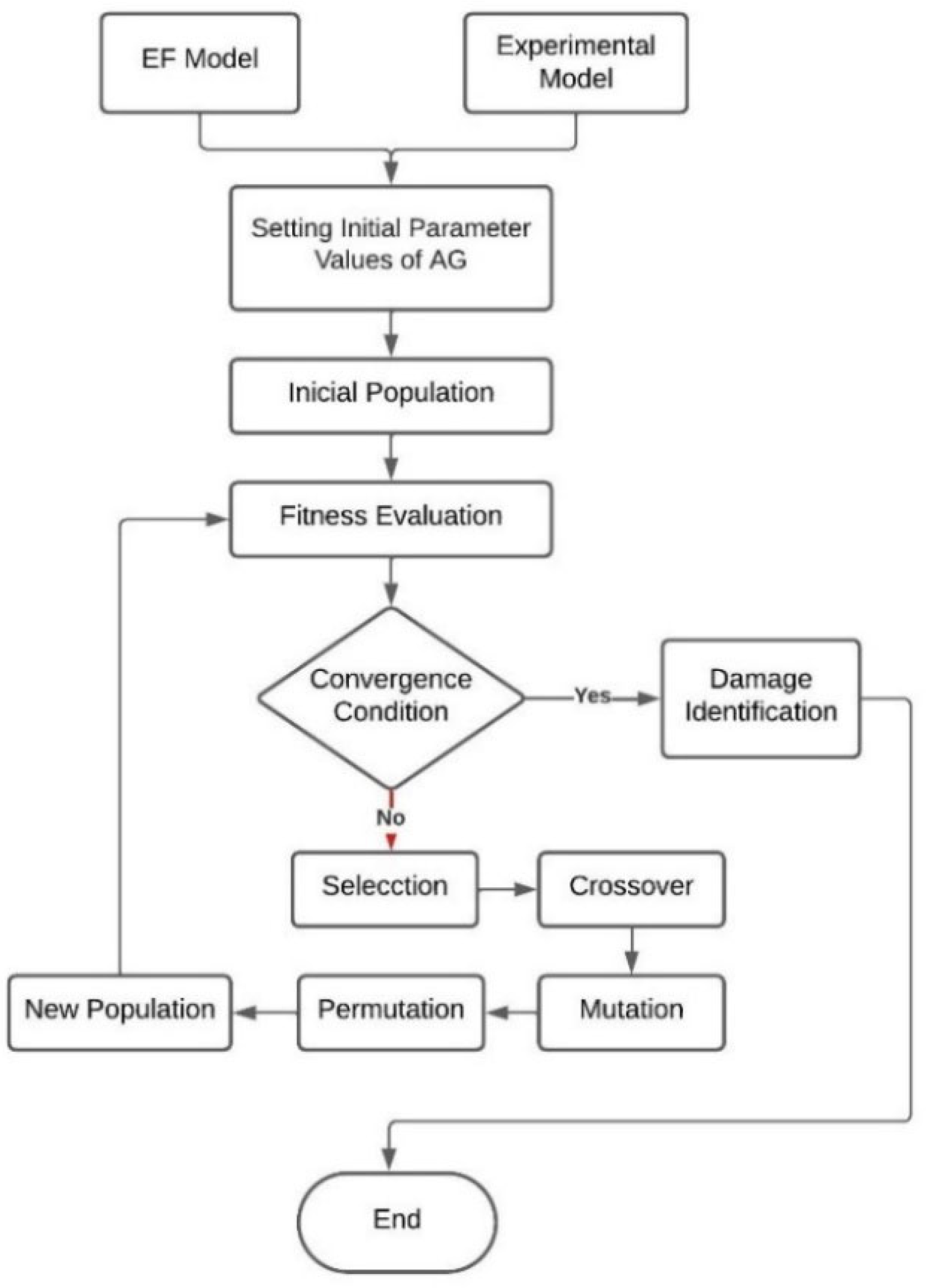
Conforming to the scheme outlined in Figure 1, the methodology starts by incorporating information from both the finite element (FE) and experimental models. Subsequently, the initial parameters of the genetic algorithm are defined, and the initial population is established. If the convergence condition is met, damage identification is accomplished. Otherwise, genetic operators (selection, crossover, mutation, and permutation) are applied to generate a new population, iterating the process until the convergence condition is satisfied. In the proposed computational methodology, each individual signifies a potential solution and is composed of chromosomes, representing the finite elements in the FE model. These chromosomes further subdivide into genes, denoting finite element properties. While various methods exist for encoding individuals, binary encoding, despite its ease of manipulation, necessitates more bits for real value representation. In contrast, real encoding incurs lower computational costs due to its more efficient bit representation.

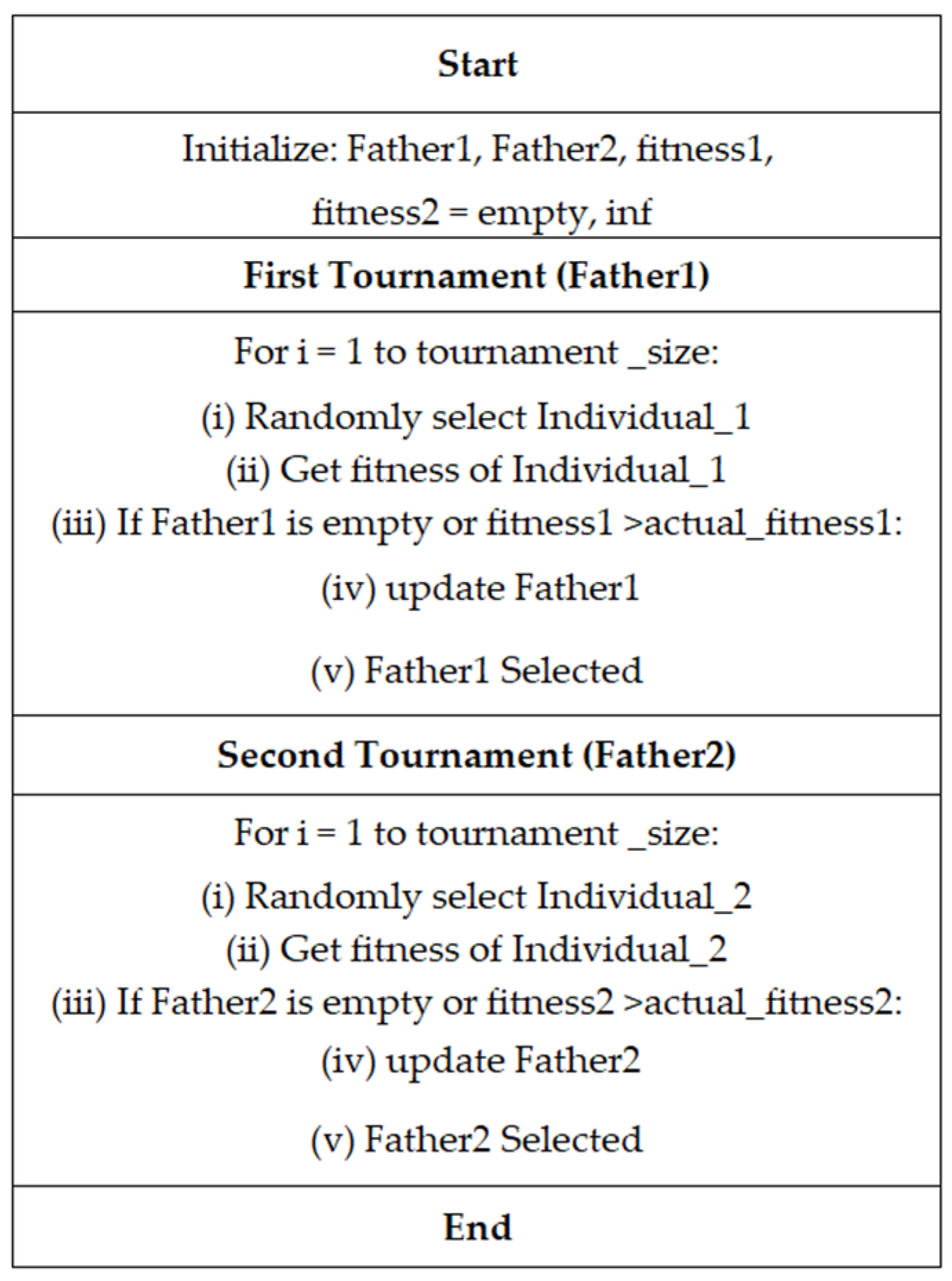
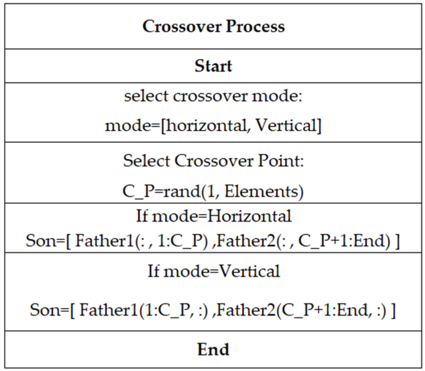
In this work, real encoding is implemented in individuals due to the simplicity of its representation and to circumvent additional computational costs. The parent selection process is carried out through a tournament and the user selects the percentage of the population that will be considered for the tournament. The process flow chart is provided in Figure 2. Conventionally, the arrangement of an individual’s chromosomes is depicted as a row vector. However, in this instance, they are organized as a column vector. This choice confers an advantage by facilitating crossover in two directions (see Figure 3), ensuring a more extensive search space for the solution.

The crossover point is randomly generated and usually occurs in a single direction (horizontal) when individuals are arranged in a row vector format. However, by organizing individuals in a column vector format, it is more feasible to introduce a crossover point in the vertical direction. This approach (see Figure 4) enables not only the crossover of finite element (FE) properties but also the elements themselves. It is important to note that the image in Figure 3 is illustrative in nature, intended to exemplify the crossing mode of individuals both horizontally and vertically. It does not aim to reflect an exact representation of the individual itself, as this is presented in Table 1.

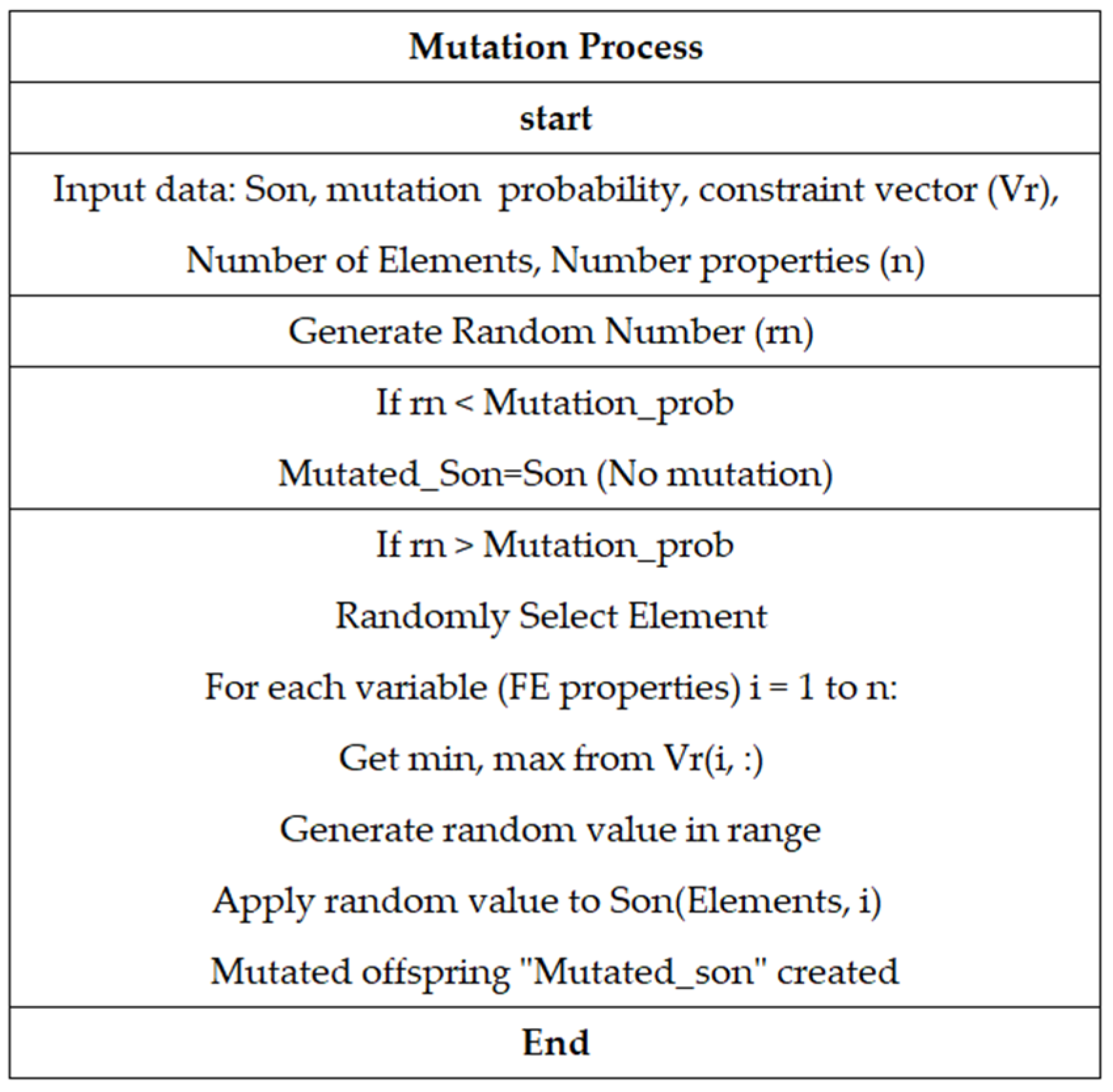
The initial population is generated through modifications (mutations) to the finite element model, with the goal of maintaining the proposed solutions within a realistic range. Furthermore, constraints are implemented in the gene mutation process to ensure that the found solution is consistent with real physical values. To achieve this, a vector of constraints or a range vector is defined. This allows the genetic algorithm (GA) to modify the properties of finite elements within physically possible values, avoiding solutions that may be mathematically feasible but lack real physical significance.

The constraint vector is defined as follows:

$${\mathit{V}}_{\mathit{r}}=\{l; \mathrm{E}; \rho ; Css\dots \}$$

(8)

$${\mathit{V}}_{\mathit{r}}=\{\left[min max\right];\left[min max\right]; \left[min max\right]; \left[min max\right]\dots \}$$

(9)

where “l” is the length of the finite element, “E” is the Young’s modulus, “$\rho$” is the material density, and “Css” is the cross-sectional area of the finite element. Constraints for each of the finite element properties are placed in this vector, which is utilized in the mutation process of individuals, as depicted in Equation (10).

$${\mathit{\chi }\mathit{m}}_{el,i}=\sum _{i=1}^{N_{var}}{\mathit{\chi }}_{el,i}\ast \left(rand\ast {\mathit{V}}_{\mathit{r}}{\left[max-min\right]}_i+{\mathit{V}}_{\mathit{r}}{\left[min\right]}_i\right)$$

(10)

where “el” and “N_var” represent the finite element to which the mutation is applied and the number of variables contained in the constraint vector, respectively, and “Rand” is a random number. The mutation process is presented in Figure 5, the constraint vector ${\mathit{V}}_{\mathit{r}}$ plays an important role in the process, and this mutation process is described by Equation (10).

The objective or fitness function is defined as an error or difference function between the FE model and the experimental model. When using vibration data, the fitness function may depend on the natural frequencies of the system, modal shapes, or both. Hong [1], in his damage detection study, employed a similar objective function (Equation (11)), initially defining it based solely on frequency data, then exclusively on modal data, and finally on a combination of both. The primary limitation of relying only on frequency shifts is the inability to differentiate damage in symmetric locations for symmetric structures, as frequencies exhibit low sensitivity to structural damage. Conversely, the drawback of using only modal data is that, while vibration modes are more sensitive to damage, in practice, the measured mode shapes tend to have relatively larger errors compared to frequency measurements.

In this study, the fitness function is constructed based on both, and it is defined as shown in Equation (11). In this equation, only those degrees of freedom that are measured are selected from the analytical mode shapes (FE), so that there is no dimension mismatch. This decision is justified in Section 4 of this paper.

In damage identification, it is essential to carefully choose the relative weights “W” assigned to frequencies and mode shapes, as these selections greatly impact the outcomes. Generally, these weights are based on the variance observed in the measurements. Since mode shapes tend to be less precise than natural frequencies, the weights for mode shapes ($W_{mj}$) are usually lower compared to those for frequencies ($W_{\lambda j}$) [1].

Additionally, these weights may be consistent across all modes or differ for each individual mode. Importantly, in the context of Equation (11), the changes in mode shapes are applied directly instead of using change ratios. This method is preferred because the smaller values of mode shapes can lead to ill-conditioning in the ratios, which could undermine the effectiveness of the damage identification process.

$$J\left({\lambda }_{x,a},{\varphi }_{x,a}\right)=\sum _{j=1}^{Nm}{W}_{\lambda j}{\left|{\displaystyle \frac{{\lambda }_{xj}-{\lambda }_{aj}}{{\lambda }_{xj}}}\right|}^2+\sum _{j=1}^{N_m}\sum _{i=1}^{N_s}{W}_{mj}{\left|{\varphi \left(i\right)}_{xj}-{\varphi \left(i\right)}_{aj}\right|}^2$$

(11)

where “$x$” and “$a$” refer to experimental and analytical data, respectively. “$N_m$” is the number of identified modes, “$N_s$” is the number of nodes where measurements were taken, and “W” is a weighting coefficient. The damage identification algorithm is implemented in MATLAB software (R2020a) following the general scheme depicted in Figure 1, incorporating the crossover type illustrated in Figure 3 and the constraint vector outlined in Equations (8) and (9). The fitness function (Equation (11)) is minimized until the defined convergence criterion is met. Upon convergence, the algorithm outputs the damaged element(s) and the damage intensity, as determined by Equation (12):

$$DI={\displaystyle \frac{K_o-K_{AG}}{K_o-K_f}}$$

(12)

where $K_o, K_{AG}$, and $K_f$ represent the initial stiffness, the stiffness determined by the genetic algorithm (GA), and the final fatigue-induced stiffness of the material, respectively. Typically, damage is represented as the difference between the initial stiffness and the one determined by the GA, without considering the material’s behavior. However, Equation (12) incorporates material behavior, including the final stiffness due to fatigue.

Considering this fatigue damage index is important when damage is caused by repeated dynamic loads, such as earthquakes. In this context, the index indicates the stage of the element’s useful life based on the percentage reduction in stiffness. For example, it is known that A36 steel exhibits a stiffness change rate with respect to the remaining life of the element, given by ΔS/Δl = −0.56 in the initial stage of damage. This implies that a 20% reduction in stiffness corresponds to a loss of 30% to 90% of the element’s useful life. In this way, there is a reference for the level of damage the structure may have incurred, according to the stiffness degradation determined by the GA (genetic algorithm) and the remaining life of the damaged element. This provides the structural evaluator with the necessary tools to decide whether to replace the damaged element or to determine if it can continue in service.

6. Case Study

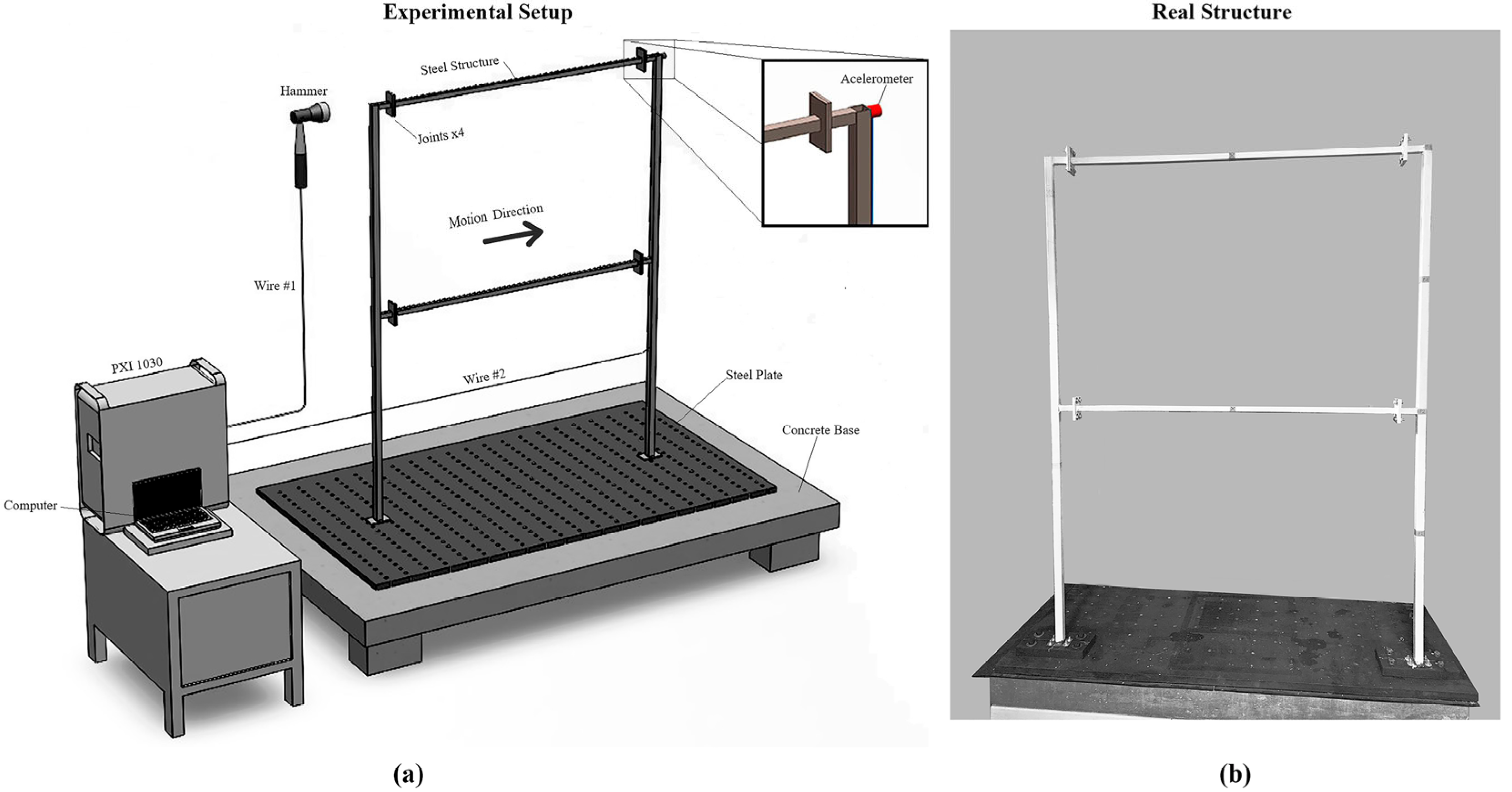
In the experimental setup (Figure 6), the steel frame consists of A36 steel columns with a length of 800 mm, featuring a square tubular cross section with dimensions b × h = 25.4 × 25.4 mm. The beams have a length of 1150 mm, a cross-sectional area of b × h = 19.05 × 19.05 mm, and a thickness of 1.9 mm for both. It is assumed that both the beams and columns have a Young’s modulus of E = 200 GPa and a density of $\rho =7850 \mathrm{k}\mathrm{m}/{\mathrm{m}}^3$.

Table 2. Defined damage scenarios for the present study.

Single Damage Scenario	Damaged Elements	Real Stiffness Reduction
SD1	1	60%
SD2	9	60%
SD3	16	60%
SD4	17	60%
Multiple Damage Scenario	Damaged Elements	Real Stiffness Reduction
MD1	1, 9	60%
MD2	18, 23	60%
MD3	1, 5, 16	60%

presents the damage scenarios used in this study, indicating the elements that are damaged a priori and the percentage reduction in the element’s stiffness. During each experiment, the sample underwent excitation using an impact hammer (model: KISTLER 9724A2A2000), while a dedicated accelerometer (model: Kistler C109004) detected the response. The accelerometer was affixed to the upper portion of the right column using a magnetic mounting base. Data acquisition was performed using a multichannel system, which recorded and analyzed both input and output signals, enabling the derivation of the frequency response function (FRF). Sampling occurred at a frequency of 500 Hz, with a resolution of 0.1 Hz. Mode shapes were subsequently identified utilizing LabView, a commercial software package.

The modal testing setup employed a multiple-input single-output (MISO) configuration, where multiple excitation points were applied while responses were recorded at a single measurement point. This approach was chosen to ensure that sufficient modal information could be captured. The excitation was applied horizontally using an impact hammer, specifically a KISTLER 9724A2A2000, as shown in Figure 6a. This configuration enabled us to excite multiple structural points to generate a more comprehensive set of frequency response functions (FRFs) across the structure.

The boundary conditions of the frame structure were carefully considered to simulate realistic constraints. The columns were modeled as fixed at the base to reflect the structural support conditions typically encountered in real-world applications. Meanwhile, the beams were rigidly connected to the columns to ensure no relative motion at the joints, thus preserving the integrity of the frame structure’s dynamic response. This setup ensures that the boundary conditions closely match those assumed in the finite element (FE) model, thus minimizing discrepancies between the numerical and experimental results.

The results obtained through the proposed computational method are presented in detail below. The method was rigorously tested under seven distinct damage scenarios designed to assess its effectiveness in both single-damage and multiple-damage cases. In each scenario, the computational algorithm was employed to identify both the location and severity of the damage based on modal and frequency data.

The experimental tests were conducted on a steel frame structure, specifically designed to simulate realistic damage conditions. To introduce controlled damage, cuts were made in selected elements of the frame using a saw. Each cut reduced the stiffness of the affected element by 60%, a reduction that was chosen based on engineering practices for simulating significant, yet non-catastrophic, damage. In the single-damage scenarios, a single cut was made in one element of the frame. In the multiple-damage scenarios, two or more elements of the frame were cut to simulate more complex damage conditions. The challenge in these cases was not only to identify the locations of the multiple damaged elements but also to assess the accuracy of the algorithm in distinguishing between varying levels of damage severity in different elements.

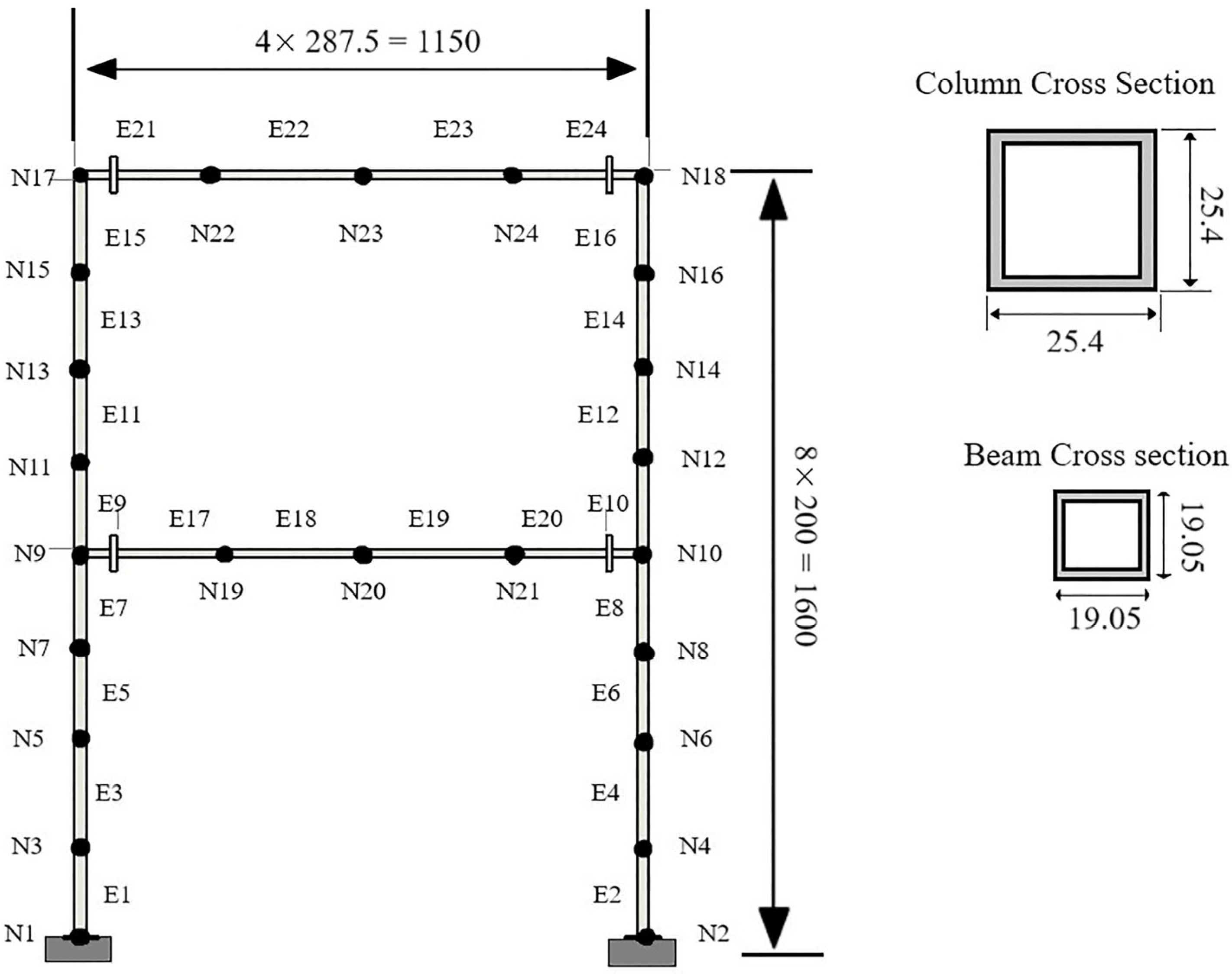
The technique of simulating damage by cutting the cross-sectional area has been employed by several authors [2,4,6,9,64,65,66] and has proved to be a simple and effective way of representing damage. In Figure 7, the steel frame used to test the proposed methodology is illustrated. Figure 7 shows the discretization into 24 elements (E1, …E24) and 24 nodes (N1, …N24), providing a clearer visual identification of the damage location.

In the finite element model, one-dimensional Euler–Bernoulli beam elements were employed, each characterized by three degrees of freedom per node, accounting for both translational and rotational movements. The mesh was discretized using 25 elements to accurately represent the structural behavior, ensuring a sufficient level of detail for the analysis. The material used in the model was considered isotropic, with a Young’s modulus of E = 200 GPa and a density of 7850 kg/m³, typical for structural steel. These material properties were chosen to reflect realistic conditions commonly found in steel structures.

The boundary conditions were applied by modeling the base of the structure with fixed supports, meaning that all degrees of freedom at the base of the columns were fully constrained, effectively preventing both translational and rotational displacements. This configuration simulates a rigid connection at the foundation, which is critical for accurately capturing the dynamic response of the structure under external loads. The choice of boundary conditions and mesh resolution was designed to balance computational efficiency with the need for precise representation of the structural behavior.

The damage identification algorithm, capable of detecting these changes in structural parameters, initiates a detailed search for damage in the structure. This procedure is essential for evaluating and understanding the structural response to alterations in parameters, thus contributing to a precise and effective identification of potential damage.

The mutation probability is set at 10 %, along with the permutation probability. Parent selection is executed through a tournament method, wherein 90 % of the population engages in competition. The crossover mode is specified as both vertical and horizontal, with respective weights of 0.9 and 0.1. These parameters were established through the recommendations in the work by Astroza [25].

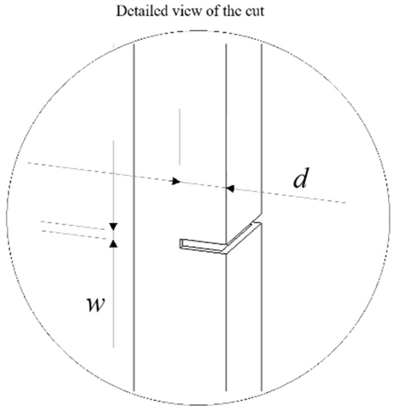
The simulated cut in the cross section of beams and columns was carried out using a saw, the dimensions of which are specified in Figure 8. This process, designed to emulate damage, resulted in a reduction in the element’s cross-sectional area and, consequently, a decrease in the stiffness (EI) of the element. This variation in stiffness directly impacts the modal parameters of the system. The relationship between stiffness and cross section was established by $\mathrm{E}(∆I)=\mathrm{E}[I_i-I_f\left(d\right)]$. Where E, $∆I$, $I_i$, $I_f,$ and d are the Young’s modulus, change in the moment of inertia, initial moment of inertia, final moment of inertia, and cutting depth. The cut configuration had a depth of 12.7 mm, which corresponded to 50% of the element’s thickness, and a width of 2.5 mm.

To achieve algorithm convergence, two conditions outlined in Equations (13) and (14) are employed. The program converges if the best fitness is under a defined limit or remains unchanged for a specified number of generations.

$$J_{best}<C_j$$

(13)

$$J_{best, i}=J_{best,i+N_{gen}}$$

(14)

where J_best represents the optimal fitness of the fitness function and C_j is a user-defined parameter indicating the minimum error between the FE model’s output and the experimental model. N_gen denotes the number of generations. In essence, the current optimal fitness is juxtaposed with the optimal fitness after N_gen to verify a discernible change; otherwise, the algorithm converges.

6.1. Single-Damage Scenario

For the case of a single instance of damage, the genetic algorithm parameters were defined as shown in

Table 3. Genetic algorithm parameters for damage scenarios.

Damage Scenario	Population	Cj	Wf	Wm
SD1	15,000	0.005	0.5	0.5
SD2	15,000	0.005	0.5	0.5
SD3	15,000	0.005	0.5	0.5
SD4	15,000	0.005	0.5	0.5

. The initial population and that of each generation were kept constant at 15,000 individuals. The minimum error, denoted as Cj, was set at 0.5 % and the weighting coefficients for natural frequencies W_f and modal shapes W_m were maintained at 50 %.

Table 4. Damage scenarios and damaged element identified.

Damage Scenario	Damaged Element	Identified Element	∆K Real	∆K Identified	Damage Index
SD1	1	1	0.6	0.61	1.01
SD2	9	9	0.6	0.72	1.19
SD3	16	16	0.6	0.7	1.17
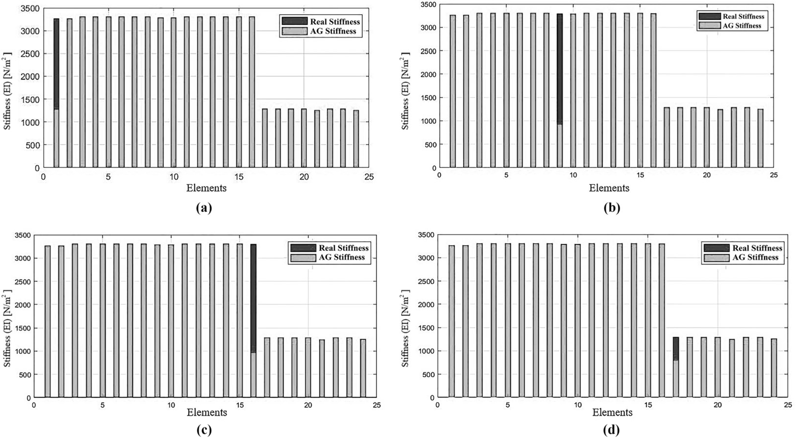
SD4	17	17	0.6	0.38	0.63

presents the results of damage scenarios, showcasing the actual damaged element alongside the element identified using a genetic algorithm (GA), as well as the real stiffness change in the element versus the identified change using the GA. The damage index (DI) is determined by the element through Equation (12), considering the degradation behavior. It is notable that a stiffness change of 60 % indicates complete damage to the element. Overall, the results are highly favorable; the algorithm adeptly identified the damaged elements without encountering false positives. Figure 9 graphically illustrates the stiffness of the structural elements; dark gray represents theoretical or actual stiffness, while light gray represents stiffness detected by the genetic algorithm (GA). The damaged element is identified by changes in element stiffness.

In Figure 9, the initial stiffness of each structural element (dark gray) is presented against the stiffness determined by genetic algorithms (light gray) after damage. It can be observed that there is a significant change in the stiffness of some elements, indicating the presence of damage in the elements exhibiting this stiffness change. It is noteworthy that the damage identification was accurate, with no apparent false positives or noise in the identification process. In

Table 5. Experimental and AG frequencies of frame.

	Experimental Frequency [Hz]			AG Frequency [Hz]
Damage Scenario	f1	f2	f3	f1	f2	f3	Σ Error %
SD1	10.9	42.8	70	10.9	43.09	70.44	1.4
SD2	11.5	42.1	70.2	11.46	41.65	70.47	1.8
SD3	11.3	44.1	66	11.36	44.07	65.92	0.7
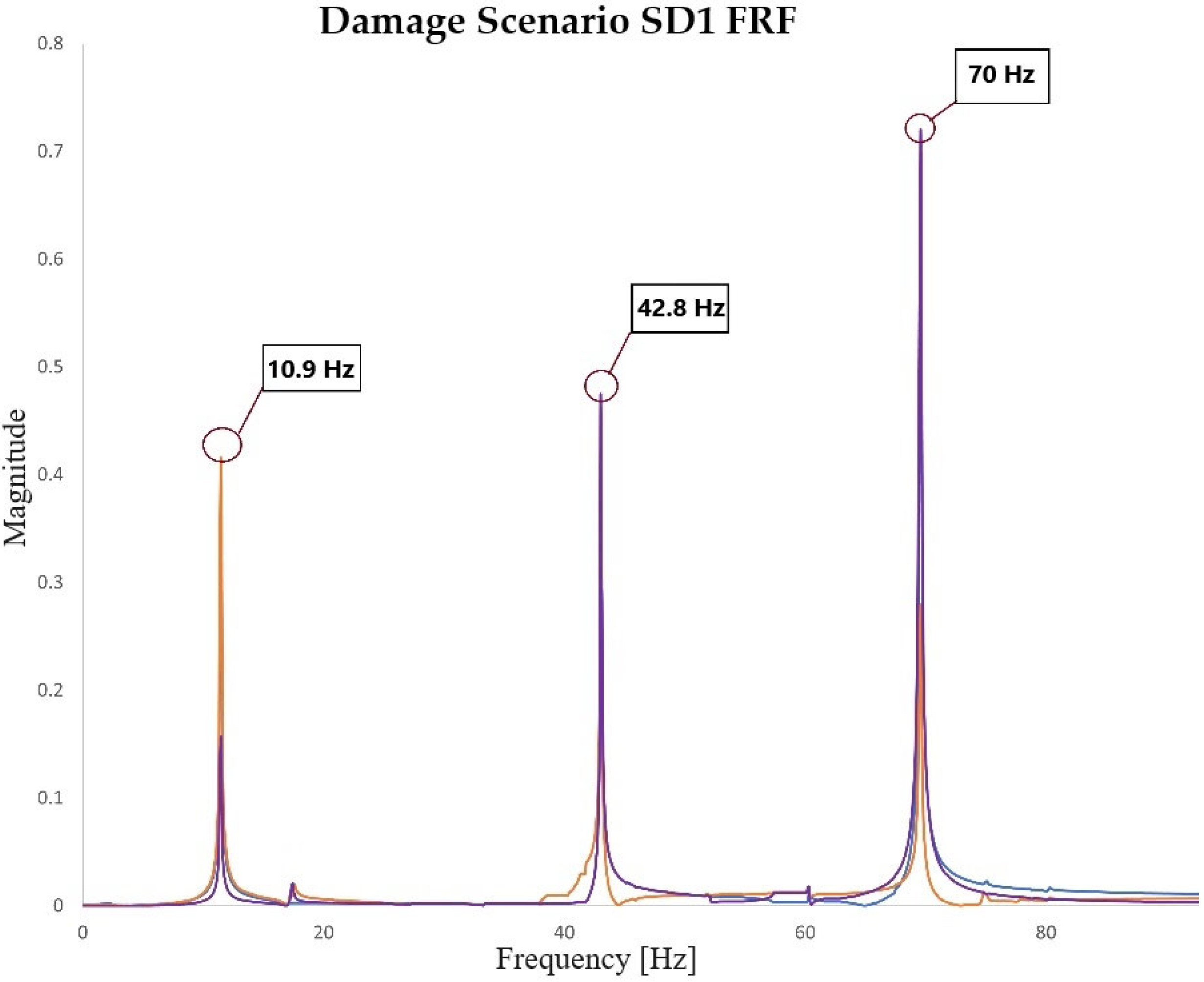
SD4	11.1	44.6	70.1	11.12	44.8	70.35	1

, the natural frequencies of the first three longitudinal modes of the frame are presented for each damage scenario. It can be observed that the variation in frequencies with respect to the damage scenario is small, highlighting the significant role of identification method sensitivity. Constructing the objective function uniquely based on frequency is not advisable, as it lacks the spatial information inherent in modal shapes. An objective function considering both parameters ensures the identification of the damage location. In Figure 10, an FRF of the damage scenario SD1 is presented.

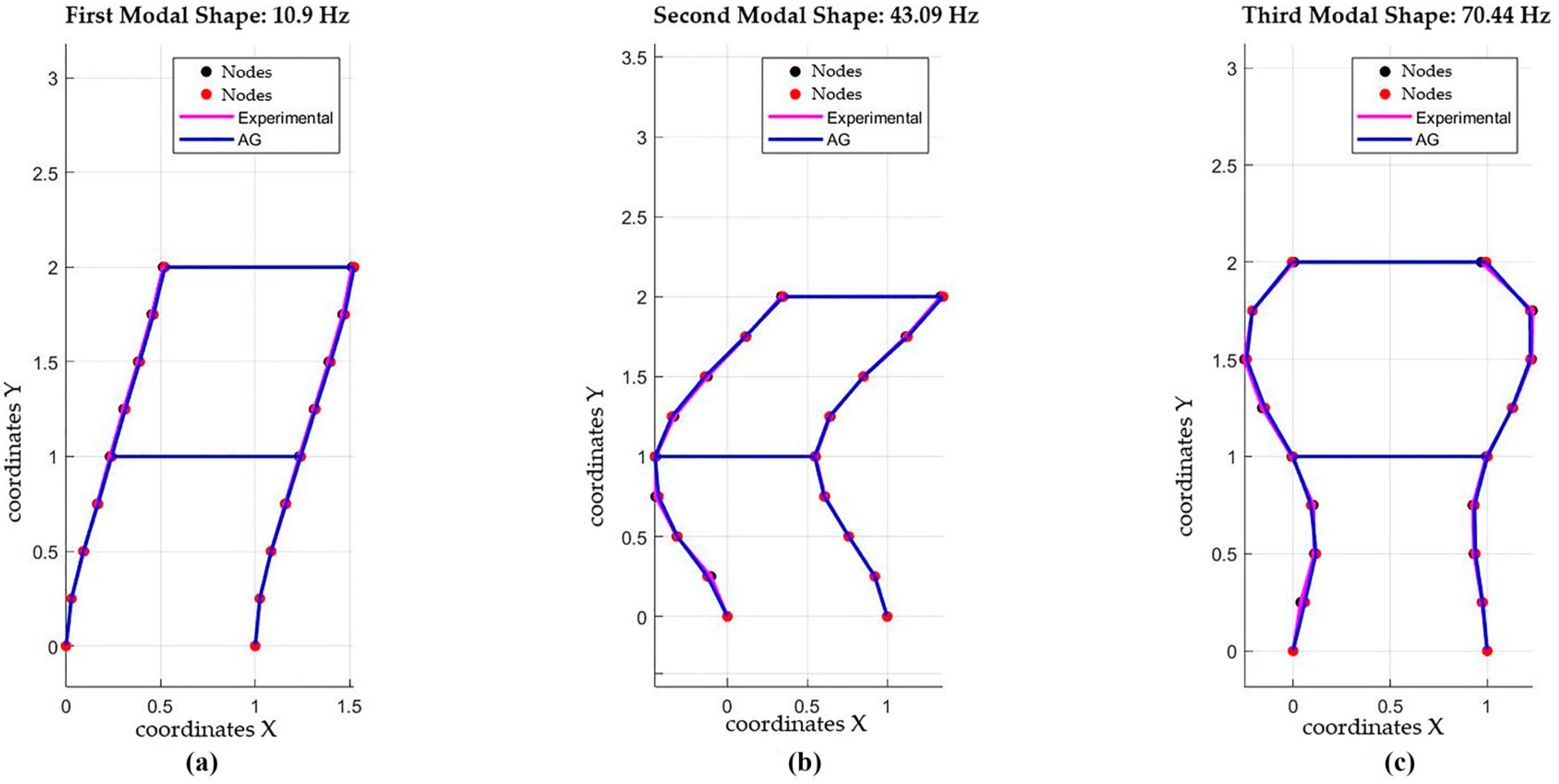
The modal shapes obtained through the modal analysis are presented in Figure 11. These modal shapes correspond to the first three vibration modes of the steel frame subjected to the damage conditions specified in Section 6 of the paper. The figures show the relative deformations of the structure in its different modal configurations, which are essential for identifying the inherent vibration patterns of the structure.

First Mode: The first vibration mode, shown in Figure 11a, features oscillation mainly in the longitudinal direction, with the largest displacements at the structure’s extremities. It has the lowest frequency and reflects the overall structural behavior.

Second Mode: Figure 11b displays a more complex second mode, with a nodal point at the center. Vibration amplitudes are higher in the middle than at the ends.

Third Mode: In Figure 11c, the third mode shows multiple nodal points and more complex displacement patterns. Deformations in this mode are highly sensitive to damage, particularly in areas with discontinuities.

These modal shapes provide critical insights into the structure’s dynamic response and are essential for damage detection. Changes in nodes and antinodes help identify areas with reduced stiffness, key to the proposed damage detection methodology.

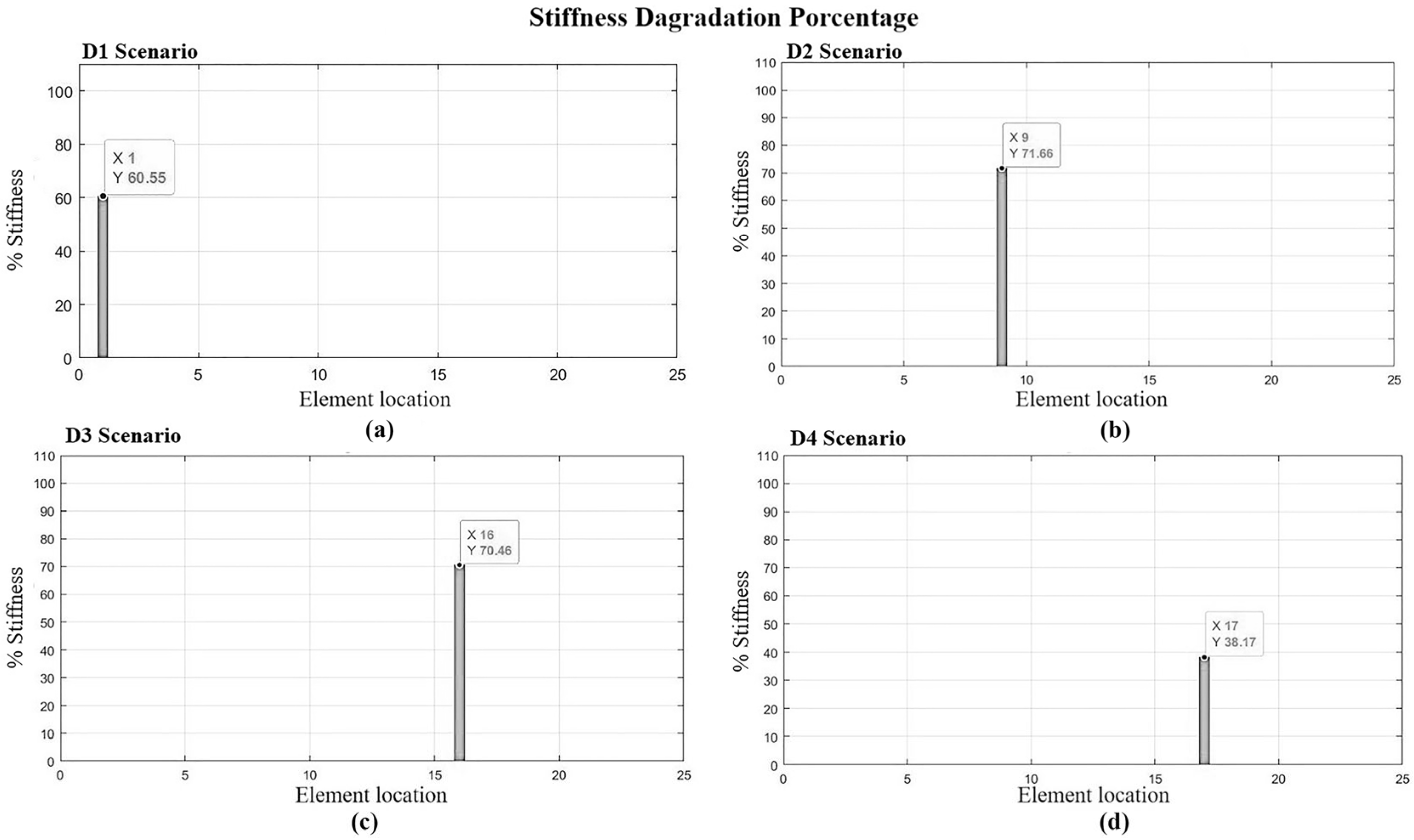
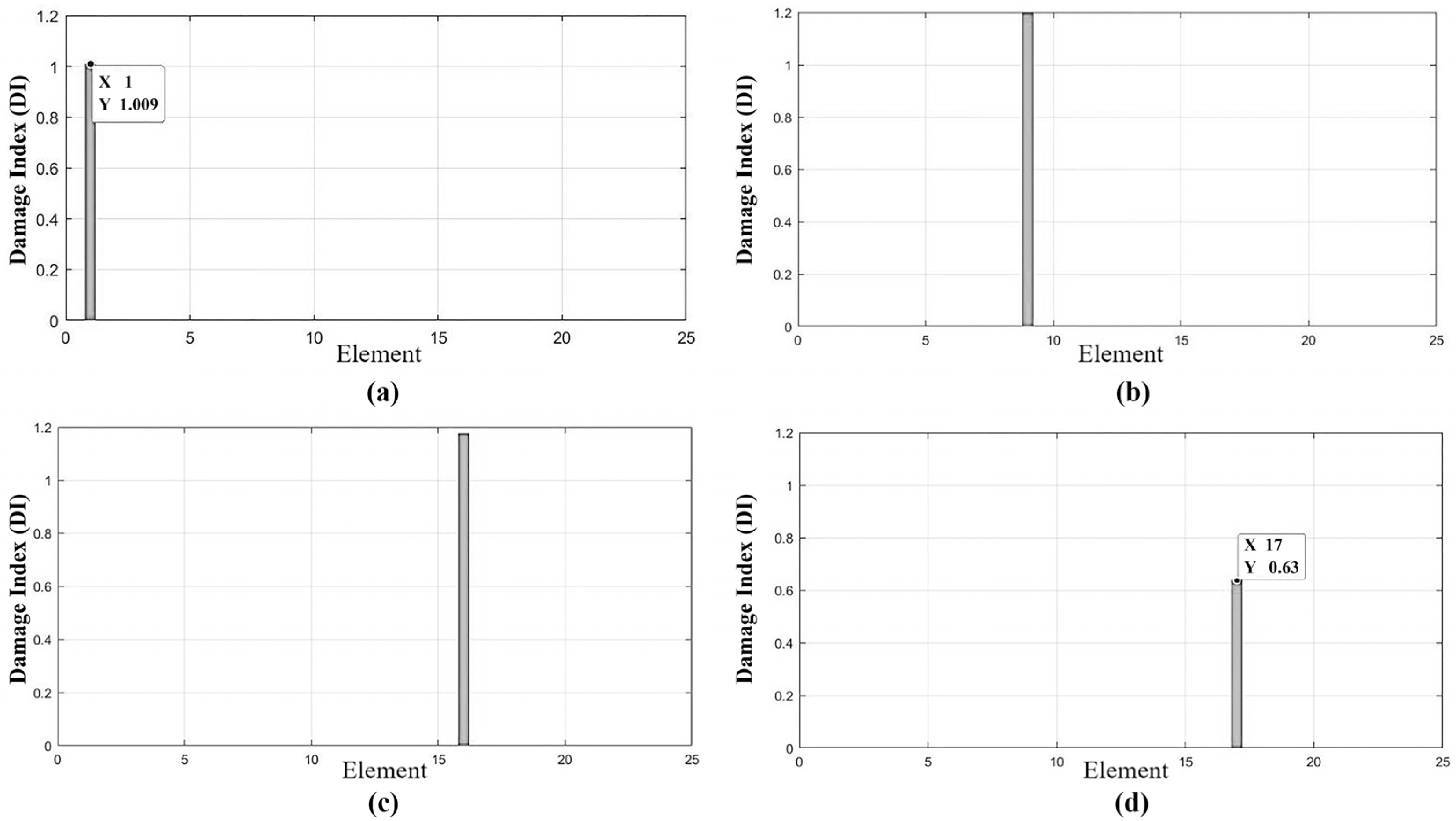
The change in stiffness (Figure 12) by itself does not fully express the state of damage in the element. However, by introducing Equation (12), which defines the element’s damage index (Figure 13) as a function of stiffness degradation behavior, we can appropriately articulate the intensity of the identified damage.

6.2. Multiple-Damage Scenario

For the case of multiple instances of damage, the genetic algorithm parameters were defined as shown in

Table 6. Genetic Algorithm parameters for damage scenarios.

Damage Scenario	Population	Cj	Wf	Wm
MD1	15,000	0.005	0.5	0.5
MD2	15,000	0.002	0.5	0.5
MD3	35,000	0.005	0.5	0.5

. The initial population and that of each generation were kept constant at 15,000 and 35,000 individuals. The minimum error, denoted as Cj, was 0.2% and the weighting coefficients for natural frequencies W_f and modal shapes W_m were 50%. In scenario DM2, a smaller difference between the Cj responses of both models was required due to the localization of the damage in the beams. The damage only affects the third mode, since the largest deformation in this mode occurs in the vertical direction, coinciding with the degradation of the flexural stiffness (EI) of the beam due to the direction of the shear.

In scenario DM3, the population size was increased because the number of elements to be identified was greater than in the other scenarios. This required a larger search space for the solution.

Table 7. Damage scenarios and damaged element identified.

Damage Scenario	Damaged Element	Identified Element	∆K Real	∆K I Identified	Damage Index
MD1	1, 9	1, 9	0.6	0.65, 0.68	1.09, 1.14
MD2	18, 23	18, 23	0.6	0.53, 0.82	0.9, 1.2
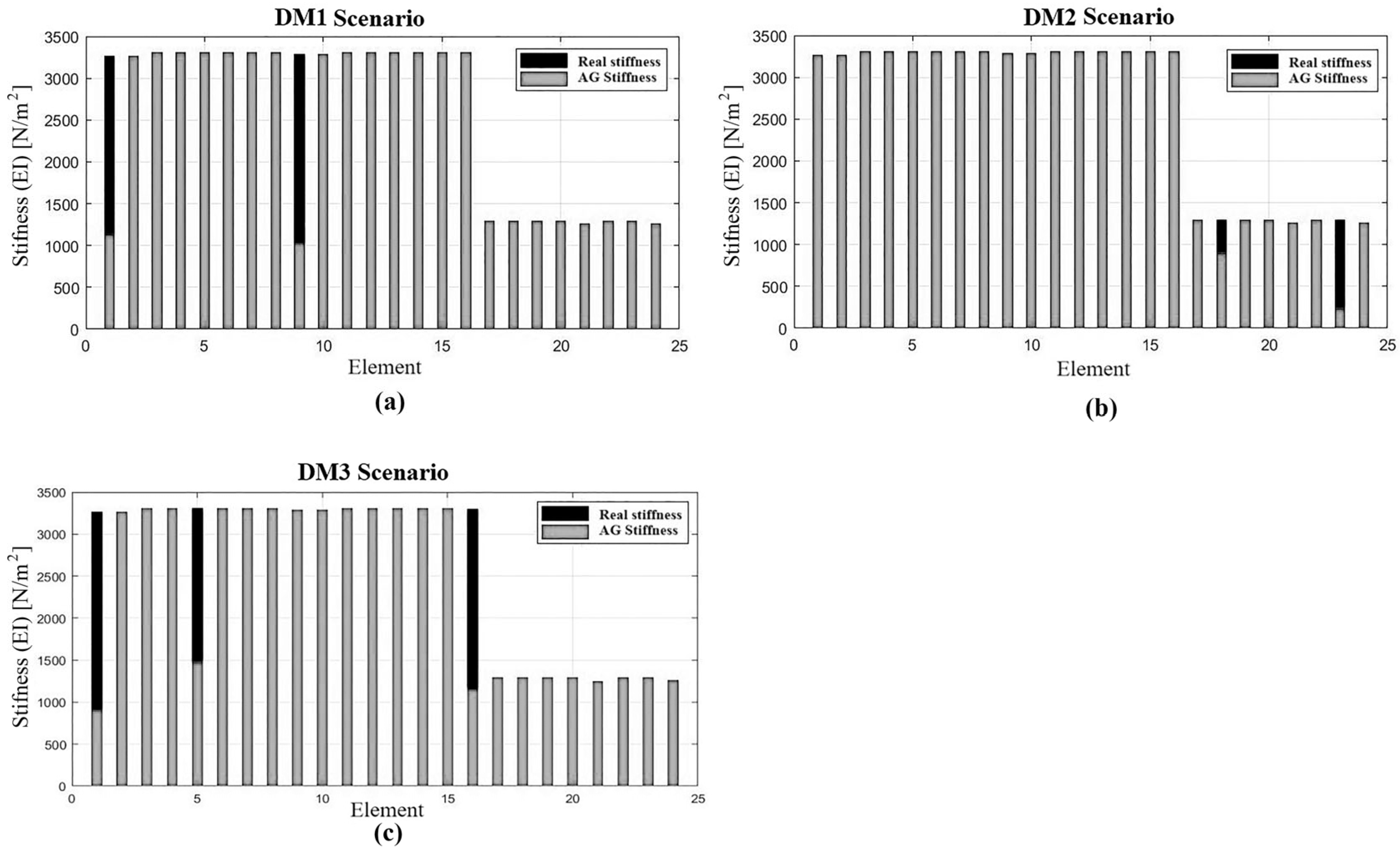
MD3	1, 5, 16	1, 5, 16	0.6	0.72, 0.6, 0.65	1.2, 0.9, 1.09

presents the results of damage scenarios in the multiple-damage case, presenting the actual damaged element beside the element identified using a genetic algorithm (GA), as well as the real stiffness change in the element versus the identified change using the GA. The damage index is determined by the element through Equation (12).

Figure 14 graphically shows the variation in stiffness of the elements identified as damaged in each damage scenario, Dark gray bars represent the initial stiffness of the elements and light gray bars represent the stiffness after the damage is detected by the GA. Table 7 and Figure 14 evidence that the identification of multiple damage was adequate and without false positives, with a change in element stiffness close to the experimental real one.

Table 8. Experimental and AG frequencies of frame on multiples damage scenarios.

	Experimental Frequency [Hz]			AG Frequency [Hz]
Damage Scenario	f1	f2	f3	f1	f2	f3	Σ Error %
MD1	10.8	40.5	70	10.71	40.13	70.3	2.6
MD2	11.5	44.4	65.3	11.49	44.34	65.27	0.2
MD3	11.7	41.5	65.4	10.58	41.71	66.5	3.2

presents the experimental frequencies obtained against those obtained by the GA. An adequate approximation to the actual system frequencies and a relative maximum cumulative error of 3.26% are observed.

If the results of Table 5 and Table 8 are observed, it can be seen that some eigenvalues increased or decreased; the observed phenomenon of increased eigenvalues despite a reduction in total stiffness can be explained by changes in mass distribution and local stiffness within the structure. When local stiffness is altered, such as through damage or modifications, the effective mass distribution can also shift, leading to variations in how vibrational energy is distributed. This change can make certain vibrational modes more prominent, effectively increasing their natural frequencies.

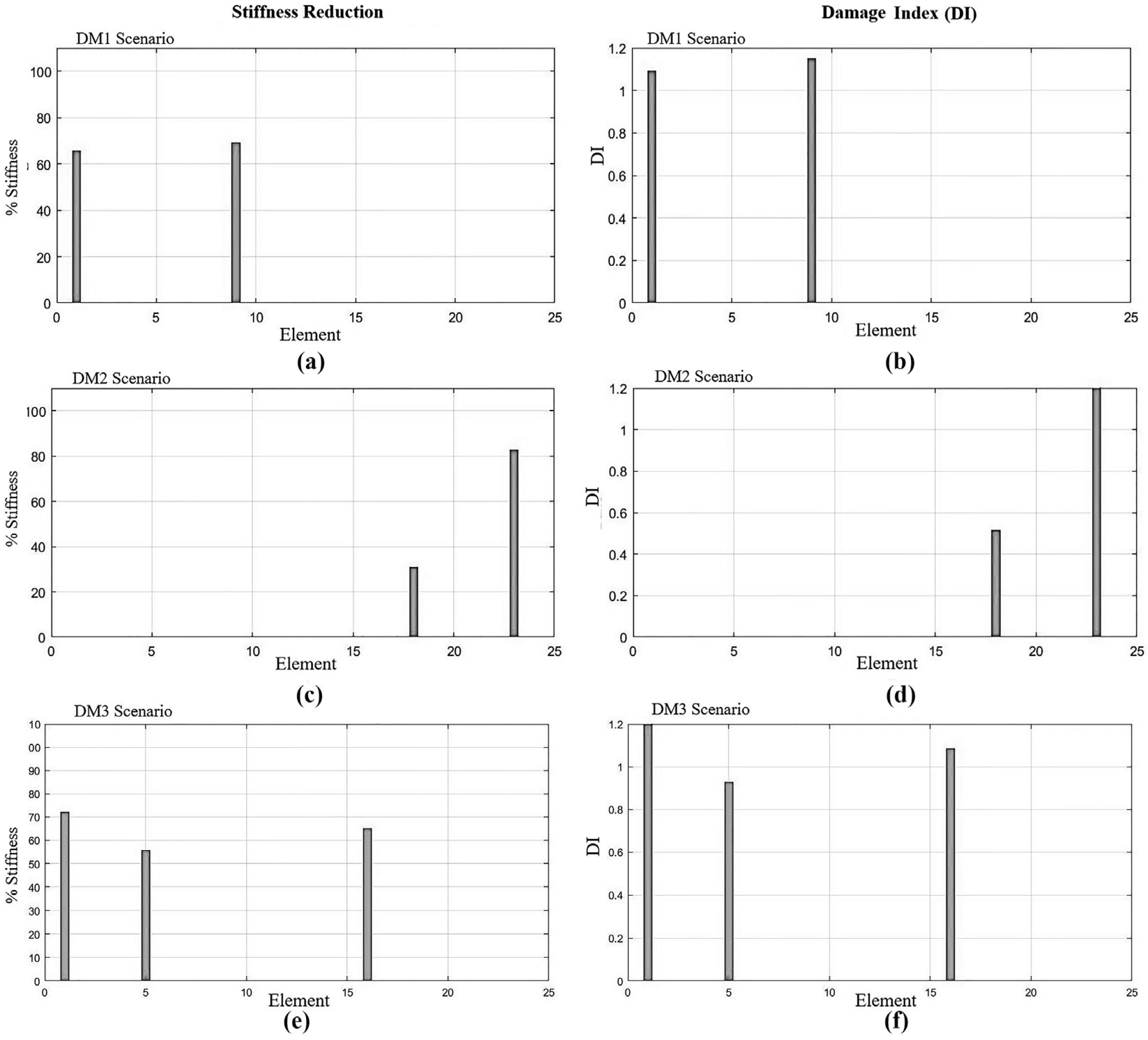
Figure 15 shows the stiffness reduction and damage index for the three damage scenarios. It can be observed that the identification of the location is correct; however, the intensity of the damage has an error rate of about 18%. In the multiple-damage scenarios, the instances of damage are located in more than one element, which makes it possible to test the algorithm’s ability to detect damage in multiple elements simultaneously and with a prediction of the change in stiffness very close to the real one. For the multiple-damage case, the parent selection, mutation, and permutation techniques of the individuals were preserved, as well as the weighting of the frequency and modal shape data. However, for the last multiple-damage case, it was necessary to increase the population of each generation. This is attributed to the increase in damaged elements, which requires a larger search space to offer better results and avoid becoming trapped in local minima.

The computation time to find the solution depends on the number of individuals per generation and the defined Cj error. On average, with a population of 15,000 and Cj = 0.005, the computation time was 25 min. Increasing the population to 35,000 with the same Cj value increased the computation time to 35 min. It is worth noting that the computation time required to find the correct solution is less than that of other computational methods reported in the literature that can take weeks with the same search space. In the case of multiple instances of damage, the algorithm showed good performance in correctly detecting the damaged elements. The damage intensity, estimated from the change in stiffness, presented small differences with respect to the real value. However, these differences remained within a range very close to the declared value. Additionally, it was observed that, by increasing the population of the algorithm, the accuracy of the prediction of damage intensity improved.

7. Conclusions

The results of this research demonstrate that the proposed computational method, by incorporating model uncertainties and using robust algorithms such as genetic algorithms (GAs), is capable of accurately identifying the location and intensity of damage, even with limited and partial modal data. Unlike traditional structural damage detection methods, which require a large amount of data, such as multiple vibration readings at different levels of the structure and several vibration modes, the approach presented here significantly reduces input data requirements. This method achieves precise results using information from a single vibration sensor and at least three vibration modes, which not only reduces instrumentation costs but also eliminates the need for expensive equipment to excite higher modes of the structure.

The ability of the method to operate with minimal input data represents a significant advance in terms of cost efficiency, as it avoids the use of multiple accelerometers, strain gauges, or other specialized sensors, which are necessary in other approaches to achieve comparable accuracy. Moreover, by considering model uncertainties, the method improves the accuracy of damage identification, avoiding false positives and providing clearer and more precise detection.

In both damage scenarios, single and multiple, the method demonstrated outstanding performance, effectively identifying the damaged elements without generating false positives. The accuracy in terms of locating damage was 100%, while that of the estimation of damage magnitude reached 80%. These results, although promising, are specific to the controlled case studies analyzed in this research (Section 6). Therefore, the generalization of this method to other structures with different geometric characteristics and damage conditions requires further analysis and validation. Future research should focus on three-dimensional analyses and the study of minimum stiffness change thresholds to further refine the methodology.

In conclusion, the proposed method offers a more cost-effective and accurate solution for structural damage detection by minimizing the required input data, reducing instrumentation costs, and allowing practical application in real structures without compromising result accuracy. However, further studies are needed to fully explore its applicability in more diverse structural scenarios.