Closed-Boundary Reflections of Shallow Water Waves as an Open Challenge for Physics-Informed Neural Networks

Abstract

Physics-informed neural networks (PINNs) have recently emerged as a promising alternative to traditional numerical methods for solving partial differential equations (PDEs) in fluid dynamics. By using PDE-derived loss functions and auto-differentiation, PINNs can recover solutions without requiring costly simulation data, spatial gridding, or time discretization. However, PINNs often exhibit slow or incomplete convergence, depending on the architecture, optimization algorithms, and complexity of the PDEs. To address these difficulties, a variety of novel and repurposed techniques have been introduced to improve convergence. Despite these efforts, their effectiveness is difficult to assess due to the wide range of problems and network architectures. As a novel test case for PINNs, we propose one-dimensional shallow water equations with closed boundaries, where the solutions exhibit repeated boundary wave reflections. After carefully constructing a reference solution, we evaluate the performance of PINNs across different architectures, optimizers, and special training techniques. Despite the simplicity of the problem for classical methods, PINNs only achieve accurate results after prohibitively long training times. While some techniques provide modest improvements in stability and accuracy, this problem remains an open challenge for PINNs, suggesting that it could serve as a valuable testbed for future research on PINN training techniques and optimization strategies.

1. Introduction

With the growing application of machine learning in Earth sciences, there is an increasing need to integrate physical constraints into model optimization. This approach enhances generalization across spatiotemporal domains with limited data and improves consistency with known physical laws expressed as partial differential equations (PDEs) [1]. The field of physics-informed machine learning addresses this through a range of applications, from purely physics-based to partially data-driven approaches [1,2]. Examples include fluid dynamics problems based on the incompressible Navier–Stokes equations [3,4,5,6,7], drag force prediction [8], advection–dispersion equations [9], and various other flow problems [10,11,12,13,14,15].

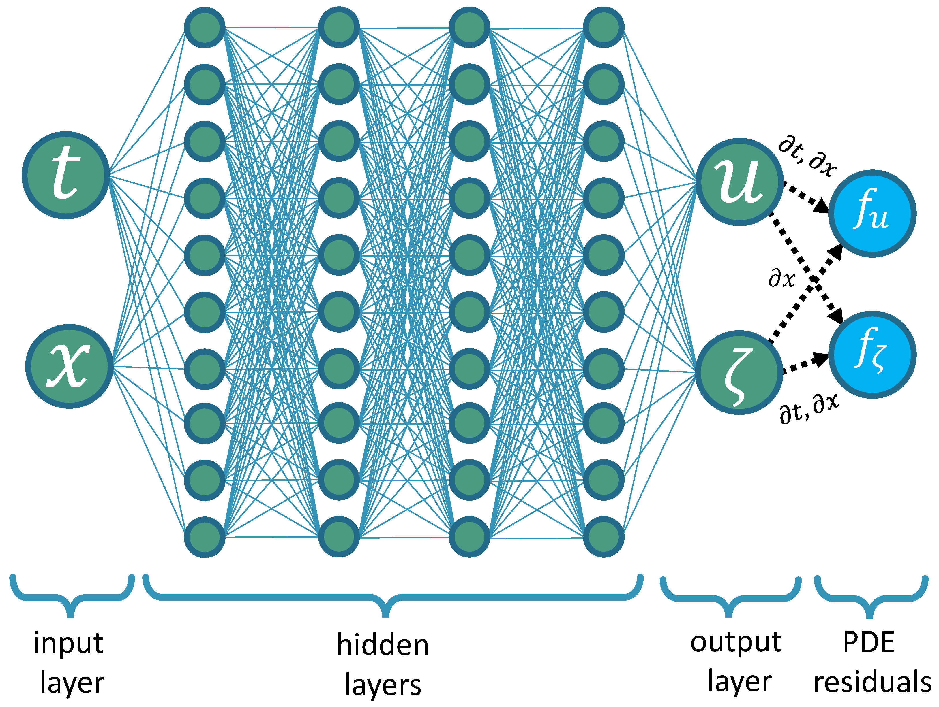
Physics-informed neural networks (PINNs) have recently gained significant attention for solving PDEs [16,17]. Several computational libraries now support automated PDE solutions using PINNs [18,19,20,21]. PINNs approximate PDE solutions by incorporating symbolic PDE representations as soft constraints in their loss functions, leveraging auto-differentiation for partial derivatives. This approach eliminates the need for costly simulation data, spatial gridding, or time discretization.

However, PINNs can exhibit slow or incomplete convergence, leading to long training times. Challenges include numerical stiffness, which can create obstructive loss landscapes [22], conflicting gradients [23,24], and imbalances in learning objectives [25,26,27,28]. Others suggest that the causality in physical systems must be respected in order to achieve fast convergence to accurate solutions [29]. Biases toward learning lower over higher frequencies and a missing propagation of initial and boundary conditions can also hinder PINN performance [30,31,32]. To address these issues, some authors suggest moving to hybrid methods that combine conventional numerical solvers [33,34,35,36], and others focus on exploring the uncertainties in the PINN approximation [37,38,39].

Numerous techniques have been developed to improve PINN convergence, including adaptive loss functions [25,40,41,42,43,44], domain decompositions [22,45,46,47], multi-scale models [48], model ensembles [49,50], reduced-order models [51], gradient projection [23,24,52], adaptive activations [53], adaptive sampling [32,54,55], hybrid differentiation schemes [34,35,36], alternative loss functions [56], and hard constraints [57,58]. Given the diversity of models and problems, evaluating their effectiveness remains challenging. Thus, standardized benchmarks are needed for physics-informed machine learning [1].

Existing PINN benchmarks focus largely on fluid dynamics [59], including test cases for Burger’s equations [60,61,62], Navier–Stokes equations [60,63], and shallow water equations (SWEs) [60,64]. SWEs are particularly useful for testing PINNs due to their ability to model diverse phenomena with relative simplicity compared to more complex systems like Navier–Stokes equations. They are particularly relevant for coastal fluid dynamics applications, such as storm surge and tsunami prediction.

Previous studies [45,64,65,66] presented accurate PINNs solutions to the 1D- and 2D-SWEs in Cartesian coordinates, as well as a test suite for atmospheric dynamics [67] in spherical coordinates, but failed to capture a critical aspect of geophysical flows: their interaction with closed boundaries. Instead, open boundaries were chosen or periodic boundary conditions were implicitly constrained by a coordinate transformation. Moreover, test cases with Cartesian coordinates only incorporated time points before the initial wave disturbance reached the domain boundary. However, the fluid behavior near domain boundaries and the transition between wet and dry regions is of high relevance to coastal modelling applications.

The ability to model reflections at closed boundaries is critical for representing phenomena such as Kelvin waves and amphidromic systems in coastal regions. Therefore, evaluating the ability of PINNs to model wave reflections is a key criterion for their suitability in geophysical fluid flow problems. Closed boundaries introduce discontinuities, making them particularly challenging for the continuous approximation of PINNs. This study assesses their ability to handle boundary interactions and their potential to handle complicated conditions in higher-dimensional systems. As shown below, we find that closed boundaries significantly challenge the efficiency of PINNs in capturing SWE solutions.

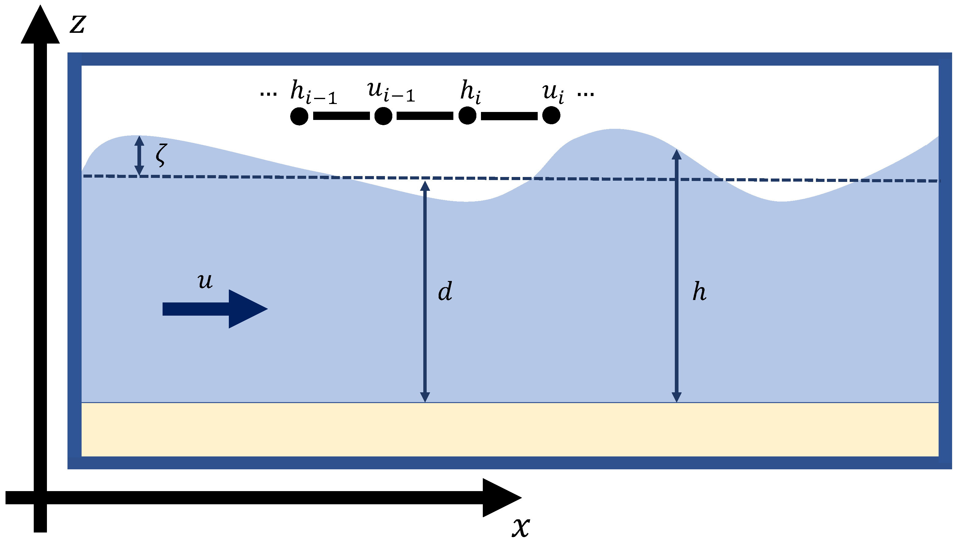
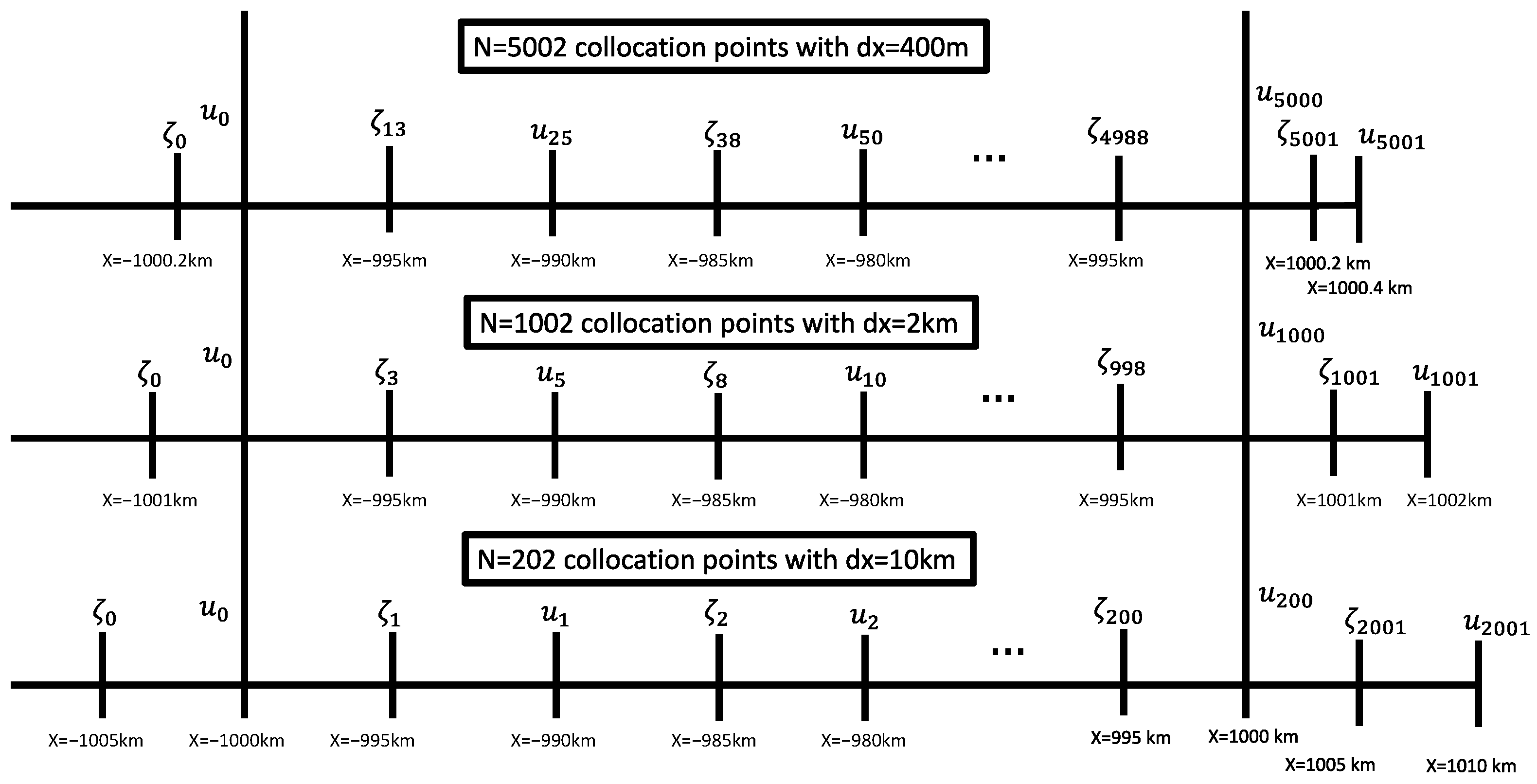
With the aim of assessing the capability of PINNs and illustrating the challenges of learning wave reflections using PINNs, we establish a new test case for physics-informed machine learning methods based on 1D shallow water equations [68] in Cartesian coordinates with closed boundaries. We carefully constructed a numerical reference solution using a semi-implicit finite difference solver. By computing the difference between numerical solutions with decreasing spatial and temporal step sizes, we estimated the uncertainty in the final reference solution. We then used this reference solution to evaluate PINNs with various architectures, optimizers, and training techniques. We tested the efficacy of non-dimensionalization, projected conflicting gradients [23,24], learning rate annealing [25], and transition functions that automatically satisfy initial and boundary conditions.

While some combinations of options and hyperparameters produced incorrect results, we found that, in several test cases, the PINNs learned the solution accurately over four wave reflections at the basin boundaries. However, the resulting trade-off between PINNs’ accuracy and the computational costs was not competitive with numerical integration. While some of the tested techniques provided minor improvements, none were able to overcome the slow convergence of PINNs. We therefore propose this problem as a suitable test case for the further development of PINNs towards Earth system modeling, specifically for coastal fluid modeling applications.

2. Materials and Methods

2.1. Physics-Informed Neural Networks

The most common type of network architectures for physics-informed neural networks [16] are fully-connected feedforward networks or multilayer perceptrons. Following the established notations [16,64], these can be expressed by a number N of transformations $f_i\left({\mathbf{v}}_{\mathbf{i}-\mathbf{1}}\right)$ that express a mapping ${\mathcal{N}}^{\mathsf{\Theta }}:{\mathbb{R}}^{d_{in}}\to {\mathbb{R}}^{d_{out}}$ from the input ${\mathbf{v}}_{\mathbf{0}}$ to the output $\mathbf{y}({\mathbf{v}}_{\mathbf{0}},\mathsf{\Theta })$ according to Equations (1) and (2). Here, the weight matrices ${\mathbf{W}}_{\mathbf{i}}$ and the bias vectors ${\mathbf{b}}_{\mathbf{i}}$ are the trainable parameters of the neural network. Together, all values in each ${\mathbf{W}}_{\mathbf{i}}$ and ${\mathbf{b}}_{\mathbf{i}}$ constitute a vector $\mathsf{\Theta }$ of network parameters to be optimized. The functions ${\mathsf{\Phi }}_i$ are typically nonlinear activation functions; in this work, they are exclusively hyperbolic tangent activation functions.

$$\begin{array}{c}\hfill {\mathbf{v}}_{\mathbf{i}}=f_i\left({\mathbf{v}}_{\mathbf{i}-\mathbf{1}}\right)={\mathsf{\Phi }}_i({\mathbf{W}}_{\mathbf{i}}{\mathbf{v}}_{\mathbf{i}-\mathbf{1}}+{\mathbf{b}}_{\mathbf{i}})\end{array}$$

(1)

$$\begin{array}{c}\hfill \mathbf{y}({\mathbf{v}}_{\mathbf{0}},\mathsf{\Theta })=(f_N\circ f_{N-1}\circ \cdots \circ f_1)\left({\mathbf{v}}_{\mathbf{0}}\right)\end{array}$$

(2)

In the network optimization or training, the network parameters $\mathsf{\Theta }$ are adapted to minimize a loss function $\mathcal{L}\left(\mathsf{\Theta }\right)$ using gradient-based optimization.

While common data-driven methods map a variable on a discretized grid from one time step to another, PINNs approximate the solutions of PDEs as continuous functions. Thus, for PINNs, the inputs are the independent variables—here, continuous space x and continuous time t—and the outputs are the dependent variables. For the 1D-SWEs, the horizontal velocity u and the sea-level elevation $\zeta$ as can be seen in Equations (3) and (4).

$$\begin{array}{c}\hfill \left[\begin{array}{c}{u}_{\mathrm{NN}}\\ {\zeta }_{\mathrm{NN}}\end{array}\right]=\left[\begin{array}{c}{y}_0\\ y_1\end{array}\right]=\mathbf{y}({\mathbf{v}}_{\mathbf{0}},\mathsf{\Theta })\end{array}$$

(3)

$$\begin{array}{c}\hfill {\mathbf{v}}_{\mathbf{0}}=\left[\begin{array}{c}t\\ x\end{array}\right]\end{array}$$

(4)

Thus, we have $d_{in}=d_{out}=2$. For example, given $N=5$ with ${\mathbf{W}}_1\in {\mathbb{R}}^{10\times 2}$, ${\mathbf{W}}_{2,3,4}\in {\mathbb{R}}^{10\times 10}$, and ${\mathbf{W}}_5\in {\mathbb{R}}^{2\times 10}$, this represents a neural network with four hidden layers and ten activations per layer. A schematic of this network architecture is depicted in Figure 1.

The basic idea of PINNs is to optimize a neural network so that its input–output function satisfies a PDE (including the initial and boundary conditions) as closely as possible. PINNs are trained by minimizing loss functions containing terms that measure violations of the PDE and its initial and boundary conditions. The initial and boundary condition losses ${\mathcal{L}}_{\mathrm{IC}}$ and ${\mathcal{L}}_{\mathrm{BC}}$ in Equations (5) and (6) describe the mean square difference between the current network approximation $u_{\mathrm{NN}}$, ${\zeta }_{\mathrm{NN}}$ and the true conditions $u_{\mathrm{IC}}$, ${\zeta }_{\mathrm{IC}}$, $u_{\mathrm{BC}}$ at their respective locations $[t_{\mathrm{IC}}=0,x_{\mathrm{IC},i}]$ and $[t_{\mathrm{BC},i},x_{\mathrm{BC}}=const.]$. Here, $N_{\mathrm{IC}}$ and $N_{\mathrm{BC}}$ denote the total number of sampling points used to evaluate the initial and boundary conditions, respectively.

$$\begin{array}{c}\hfill {\mathcal{L}}_{\mathrm{IC}}={\displaystyle \frac{1}{N_{\mathrm{IC}}}}{\mathsf{\Sigma }}_{i=1}^{N_{\mathrm{IC}}}{[u_{\mathrm{IC}}\left(x_{\mathrm{IC},i}\right)-u_{\mathrm{NN}}(t=0,x_{\mathrm{IC},i})]}^2\\ \hfill +{\displaystyle \frac{1}{N_{\mathrm{IC}}}}{\mathsf{\Sigma }}_i^{N_{\mathrm{IC}}}{[{\zeta }_{\mathrm{IC}}\left(x_{\mathrm{IC},i}\right)-{\zeta }_{\mathrm{NN}}(t=0,x_{\mathrm{IC},i})]}^2\end{array}$$

(5)

$$\begin{array}{c}\hfill {\mathcal{L}}_{\mathrm{BC}}={\displaystyle \frac{1}{N_{\mathrm{BC}}}}{\mathsf{\Sigma }}_{i=1}^{N_{\mathrm{BC}}}{[u_{\mathrm{BC}}\left(t_{\mathrm{BC},i}\right)-u_{\mathrm{NN}}(t_{\mathrm{BC},i},x=x_{\mathrm{BC}})]}^2\end{array}$$

(6)

Violations of the PDE itself are quantified by applying automatic differentiation to compute partial derivatives of the network outputs $u_{\mathrm{NN}},{\zeta }_{\mathrm{NN}}$ with respect to the inputs $x,t$. This requires a differentiable input–output function. The PDE loss ${\mathcal{L}}_{\mathrm{PDE}}$ in Equation (7) is then the sum of mean squares of the individual PDE residuals $f_u$ and $f_{\zeta }$ at some collocation points $[t_{\mathrm{PDE},i},x_{\mathrm{PDE},i}]$. Accordingly, $N_{\mathrm{PDE}}$ refers to the total number of sampling points for evaluating the PDE residuals.

$$\begin{array}{c}\hfill {\mathcal{L}}_{\mathrm{PDE}}={\mathcal{L}}_{\mathrm{PDE},u}+{\mathcal{L}}_{\mathrm{PDE},\zeta }\\ \hfill ={\displaystyle \frac{1}{N_{\mathrm{PDE}}}}{\mathsf{\Sigma }}_i^{N_{\mathrm{PDE}}}\left[f_u^2(x_{\mathrm{PDE},i},t_{\mathrm{PDE},i})\right]\\ \hfill +{\displaystyle \frac{1}{N_{\mathrm{PDE}}}}{\mathsf{\Sigma }}_i^{N_{\mathrm{PDE}}}\left[f_{\zeta }^2(x_{\mathrm{PDE},i},t_{\mathrm{PDE},i})\right]\end{array}$$

(7)

Lastly, all three parts of the loss function are summarized with a respective weight $w_{\mathrm{PDE}}$, $w_{\mathrm{IC}}$ and $w_{\mathrm{BC}}$ to compute the total loss ${\mathcal{L}}_{\mathrm{total}}$ in Equation (8). If not otherwise specified, we set $w_{\mathrm{PDE}}=w_{\mathrm{IC}}=w_{\mathrm{BC}}=1$ for the equal consideration of each term.

$$\begin{array}{c}\hfill {\mathcal{L}}_{\mathrm{total}}=w_{\mathrm{PDE}}{\mathcal{L}}_{\mathrm{PDE}}+w_{\mathrm{IC}}{\mathcal{L}}_{\mathrm{IC}}+w_{\mathrm{BC}}{\mathcal{L}}_{\mathrm{BC}}\end{array}$$

(8)

Recent PINN studies identified three main sources of errors (Figure 2) [45,69]. First, in the optimization process, it is not guaranteed that the optimizer will converge to its global minimum. This introduces an optimization error, given by the difference in accuracy between the approximation after training and the global optimum. Second, the limited accuracy with which even optimal parameters for the network architecture could produce the true PDE solution leads to approximation errors. Third, when a finite number of collocation points $(x_i,t_i)$ are used to minimize the loss function, the network can over-fit on these points, leading to an estimation error [69]. Using more control points decreases over-fitting, which leads to better generalization [70].

2.2. The Shallow Water Equations

The shallow water equations describe a specific case of the Navier–Stokes equations with a fluid layer of constant density under the hydrostatic approximation [68]. In this approximation, the horizontal momentum equations and the continuity equation fully describe the fluid motion. For the 1D case, the fluid motion can be obtained using Equations (9) and (10), respectively. Their applications in Cartesian coordinates, as considered here, range from regional flood [71,72], tsunami propagation [73,74] and storm surge [75,76] models to more localized river flow and sediment transport models [77]. Efficient, reliable, and accurate predictions for extreme events such as storm surges, floods, and tsunamis are essential for early warning systems for populations in coastal areas.

A variety of numerical methods have been developed for solving geophysical fluid modeling applications. For the SWE, numerical models employ different spatial discretization schemes, including finite difference, finite volume, finite element, and spectral methods, along with predominantly semi-implicit time integration schemes, for modeling water bodies [78,79,80,81]. For atmospheric models, however, explicit schemes are common [82]. More recently, discontinuous Galerkin methods have gained attention as a robust approach to solving the shallow water equations [83]. Due to the inefficiency of discrete methods in simulating coupled phenomena on vastly different time and space scales, there has been extensive work on developing tailored discretizations and computational grids [84]. This motivates the development of continuous, gridless methods such as PINNs.

PINNs have shown promising results in mathematical test problems as well as fluid modeling problems [3,16,59]. For more complex hydrodynamic or atmospheric modelling applications, however, their ability to represent relevant phenomena and dynamics is less clear. With this study, we therefore aim to facilitate the development of physics-informed machine learning methods towards more complex applications based on shallow water equations as well as other geophysical fluid dynamics applications.

2.3. Initial-Boundary Value Problem

We solved the 1D shallow water equations (SWE, Equations (9) and (10)) with a flat bottom topography [68]. Here, u is the horizontal velocity, $h=d+\zeta$ is the fluid layer thickness with undisturbed thickness $d=const$, and the sea-level elevation is $\zeta$. The parameter g is the gravitational acceleration constant and $A_H$ is the horizontal diffusivity.

$$\begin{array}{c}\hfill f_u:={\displaystyle \frac{\partial u}{\partial t}}+g{\displaystyle \frac{\partial \zeta }{\partial x}}+u{\displaystyle \frac{\partial u}{\partial x}}-A_H{\displaystyle \frac{{\partial }^{2}u}{\partial x^2}}=0\end{array}$$

(9)

$$\begin{array}{c}\hfill f_{\zeta }:={\displaystyle \frac{\partial \zeta }{\partial t}}+u{\displaystyle \frac{\partial \zeta }{\partial x}}+h{\displaystyle \frac{\partial u}{\partial x}}=0\end{array}$$

(10)

As a new test case, we propose an initial-boundary value problem based on Equations (9) and (10) with the following parameter settings: $d=100\mathrm{m}$, $g=9.81{\mathrm{ms}}^{-2}$ and $A_H=0$ or $5\times {10}^4{\mathrm{m}}^2{\mathrm{s}}^{-1}$, respectively. The spatiotemporal domain is within the intervals $x\in [-L,L]$ and $t\in [0,75\mathrm{h}]$, where $L={10}^3\mathrm{km}$, as used below. We use the closed boundary conditions expressed in Equation (11), meaning that the velocity is zero at the domain boundaries. Initially, the horizontal velocity field u in Equation (12) is set to zero and the sea-level elevation assumes a Gaussian bell shape at the domain center ($\mu =0$) with width $\sigma =100\mathrm{km}$.

$$\begin{array}{c}\hfill u(x=L,t)=u(x=-L,t)=0\end{array}$$

(11)

$$\begin{array}{c}\hfill u(x,t=0)=0\end{array}$$

(12)

$$\begin{array}{c}\hfill \zeta (x,t=0)={\displaystyle \frac{2.5}{\sqrt{2\pi }}}exp\left(-0.5{\left({\displaystyle \frac{x-\mu }{\sigma }}\right)}^2\right)\end{array}$$

(13)

The conceptual setup is depicted schematically in Figure 3, with the positive z-axis pointing upwards.

2.4. Training Setup

Here, we describe the specific model and training configurations for the PINN-based model optimization. The methods described in this section are used in the default training setup, while those described in the next section were tested as optional modifications.

Non-dimensionalization: For the model optimization, we minimize an objective function incorporating the penalty terms for the violations of the PDEs and the initial and boundary conditions for both u and $\zeta$. For effective optimization, it is essential that these terms do not vary by many orders of magnitude, as this would lead to some terms dominating others. For the SWE, this problem is apparent when considering the scales of u and $\zeta$, as well as the difference in horizontal and vertical scales. In the given initial-boundary value problem, u is approximately one order of magnitude smaller than $\zeta$. An effective way to counteract this is through the non-dimensionalization of the PDEs. For each spatial and temporal dimension, a characteristic reference scale is chosen that is representative of the domain size and phenomena. Then, all variables and derivatives are scaled by their respective reference scale to obtain the dimensionless variables and derivatives. The non-dimensionalized variables, derivatives, and constants indicated by the hat are defined in Equations (14) and (15). Here, the characteristic horizontal and vertical length scales are L and H and the characteristic time scale is T, as defined in Equation (16). The definition of the vertical scale as a function of the horizontal length scale and the time scale was adapted from previous work [45]. Parameter c can be chosen to adjust the ratio between vertical and horizontal length scales. For all the experiments presented below, $c=1$ was chosen.

$$\begin{array}{c}\hfill \widehat{x}={\displaystyle \frac{x}{L}},\widehat{t}={\displaystyle \frac{t}{T}},\widehat{u}={\displaystyle \frac{u}{U}}=u{\displaystyle \frac{T}{L}},\widehat{h}={\displaystyle \frac{h}{H}},\\ \hfill \widehat{\zeta }={\displaystyle \frac{\zeta }{H}},\widehat{d}={\displaystyle \frac{d}{H}},\widehat{g}=g{\displaystyle \frac{T^2}{H}}{\widehat{A}}_H=A_H{\displaystyle \frac{T}{L^2}}\end{array}$$

(14)

$$\begin{array}{c}\hfill {\displaystyle \frac{\partial }{\partial x}}={\displaystyle \frac{\partial }{\partial \widehat{x}}}{\displaystyle \frac{\partial \widehat{x}}{\partial x}}={\displaystyle \frac{1}{L}}{\displaystyle \frac{\partial }{\partial \widehat{x}}},{\displaystyle \frac{\partial }{\partial t}}={\displaystyle \frac{\partial }{\partial \widehat{t}}}{\displaystyle \frac{\partial \widehat{t}}{\partial t}}={\displaystyle \frac{1}{T}}{\displaystyle \frac{\partial }{\partial \widehat{t}}}\end{array}$$

(15)

$$\begin{array}{c}\hfill L={10}^3\mathrm{km},T=1\mathrm{day}\mathrm{and}H=c{\displaystyle \frac{L^2}{g{T}^2}}\end{array}$$

(16)

Inserting the dimensionless variables and derivatives into Equations (9) and (10) and simplifying them, we obtain the dimensionless form of the 1D-SWE given by Equations (17) and (18).

$$\begin{array}{c}\hfill {\widehat{f}}_{\widehat{u}}:={\displaystyle \frac{\partial \widehat{u}}{\partial \widehat{t}}}+c{\displaystyle \frac{\partial \widehat{h}}{\partial \widehat{x}}}+\widehat{u}{\displaystyle \frac{\partial \widehat{u}}{\partial \widehat{x}}}-{\widehat{A}}_H{\displaystyle \frac{{\partial }^2\widehat{u}}{\partial {\widehat{x}}^2}}=0\end{array}$$

(17)

$$\begin{array}{c}\hfill {\widehat{f}}_{\widehat{\zeta }}:={\displaystyle \frac{\partial \widehat{\zeta }}{\partial \widehat{t}}}+\widehat{u}{\displaystyle \frac{\partial \widehat{h}}{\partial \widehat{x}}}+\widehat{h}{\displaystyle \frac{\partial \widehat{u}}{\partial \widehat{x}}}=0\end{array}$$

(18)

The terms ${\widehat{f}}_{\widehat{u}}$ and ${\widehat{f}}_{\widehat{\zeta }}$ then replace $f_u$ and $f_{\zeta }$ in Equation (7) to evaluate the violation of the PDEs. After training, the network output is re-dimensionalized for comparison to the numerical solution. Initial experiments without non-dimensionalization failed to converge to PDE solutions.

Mini batch gradient descent: The collocation points for the local minimization of the individual loss terms ${\mathcal{L}}_{\mathrm{PDE}}$, ${\mathcal{L}}_{\mathrm{BC}}$ and ${\mathcal{L}}_{\mathrm{IC}}$ are sampled at random once at the model initialization using Latin hypercube sampling [86]. For each training step, however, mini batches with one percent of the points are considered for the gradient step. This means that, for each epoch, one hundred gradient steps are taken.

Projected conflicting gradients: An optimization problem with a loss function consisting of several learning objectives, such as Equation (8), is called a multi-task learning problem. In general, minimizing the sum of the objectives is not guaranteed to minimize each individual learning objective, and the different objectives may provide conflicting gradients for the parameter updates. To address this problem, a projection of conflicting gradients (PCGrad) was previously developed [23,24] that has been shown to improve optimization results in certain scenarios involving highly conflicting gradients (i.e., an angle $\mathsf{\Phi }>{90}^{\circ }$ between the gradients), high curvature in the objective function, and high learning rates. The gradient projection is illustrated in Figure 4.

2.5. Additional Methods

In this section, we describe two additional modifications to our model architecture and training setup, which we tested in further experiments to determine whether they would increase the quality or speed of convergence.

Learning rate annealing: An alternative to PCGrad that could prevent a single term of the composite loss function ${\mathcal{L}}_{\mathrm{total}}$ from being dominated by one of the loss terms is adapting the weights $w_{\mathrm{PDE}}$, $w_{\mathrm{BC}}$ and $w_{\mathrm{IC}}$ during training to balance the individual contributions. One way of dynamically updating these weights during the optimization, based on the gradient statistics, has been described in a previous study [25]. This approach is termed Learning Rate Annealing (LRA). When using LRA, we use the hyperparameter setting $a=0.9$ as suggested for similar applications [64].

Transition functions: Physics-informed neural networks use separate loss terms for the violation of the PDEs and the initial and boundary conditions. When all three loss terms are low everywhere, an accurate PDE solution has been learned. However, if violations of the PDE or its initial or boundary conditions occur at an early time point, the error may propagate to later times even without further violations of the PDE. One way to address the challenge presented by this potential accumulation of errors is to introduce hard constraints to the initial or boundary conditions. In order to strictly enforce the initial or boundary conditions, we applied transition functions to the network output $\mathbf{y}$ in Equation (1) in some experiments. For these cases, u and $\zeta$ were not directly obtained from $\mathbf{y}$, but were instead obtained using one of three different formulas ${\mathcal{T}}_1\left(\mathbf{y}\right)$, ${\mathcal{T}}_2\left(\mathbf{y}\right)$ or ${\mathcal{T}}_3\left(\mathbf{y}\right)$, as described in Equations (19)–(22).

$$\begin{array}{c}\hfill \left[\begin{array}{c}{u}_{\mathrm{NN}}\\ {\zeta }_{\mathrm{NN}}\end{array}\right]={\mathcal{T}}_1\left(\mathbf{y}\right)=\left[\begin{array}{c}{\mathcal{T}}_{u,1}\left(y_0\right)\\ {\mathcal{T}}_{\zeta ,1}\left(y_1\right)\end{array}\right]\\ \hfill =\left[\begin{array}{c}{y}_0\mathsf{\Psi }\left({\displaystyle \frac{x_{\max }-x}{{\tau }_x}}\right)\mathsf{\Psi }\left({\displaystyle \frac{x+x_{\max }}{{\tau }_x}}\right)\\ y_1\end{array}\right]\end{array}$$

(19)

$$\begin{array}{c}\hfill \left[\begin{array}{c}{u}_{\mathrm{NN}}\\ {\zeta }_{\mathrm{NN}}\end{array}\right]={\mathcal{T}}_2\left(\mathbf{y}\right)=\left[\begin{array}{c}{\mathcal{T}}_{u,2}\left(y_0\right)\\ {\mathcal{T}}_{\zeta ,2}\left(y_1\right)\end{array}\right]\\ \hfill =\left[\begin{array}{c}{y}_0\mathsf{\Psi }\left({\displaystyle \frac{x_{\max }-x}{{\tau }_x}}\right)\mathsf{\Psi }\left({\displaystyle \frac{x+x_{\max }}{{\tau }_x}}\right)\mathsf{\Psi }\left({\displaystyle \frac{t}{{\tau }_t}}\right)\\ h_{0}exp\left({\displaystyle \frac{-t}{{\tau }_t}}\right)+y_1\mathsf{\Psi }\left({\displaystyle \frac{t}{{\tau }_t}}\right)\end{array}\right]\end{array}$$

(20)

$$\begin{array}{c}\hfill \left[\begin{array}{c}{u}_{\mathrm{NN}}\\ {\zeta }_{\mathrm{NN}}\end{array}\right]={\mathcal{T}}_3\left(\mathbf{y}\right)=\left[\begin{array}{c}{\mathcal{T}}_{u,3}\left(y_0\right)\\ {\mathcal{T}}_{\zeta ,3}\left(y_1\right)\end{array}\right]\\ \hfill =\left[\begin{array}{c}{y}_0\mathsf{\Psi }\left({\displaystyle \frac{x_{\max }-x}{{\tau }_x}}\right)\mathsf{\Psi }\left({\displaystyle \frac{x+x_{\max }}{{\tau }_x}}\right)\mathsf{\Psi }\left({\displaystyle \frac{t}{{\tau }_t}}\right)\\ h_0+y_1\mathsf{\Psi }\left({\displaystyle \frac{t}{{\tau }_t}}\right)\end{array}\right]\end{array}$$

(21)

$$\begin{array}{c}\hfill \mathsf{\Psi }\left(z\right)=1-exp(-z)\end{array}$$

(22)

The parameters ${\tau }_x$ and ${\tau }_t$ are used to optimize the approximation ability of the model and are given by ${\tau }_x=0.1\times x_{\max }$ and ${\tau }_t=0.1\times t_{\max }$. If non-dimensionalization is applied, the parameters are scaled by the reference scales such that $t_{\max }=3.125$ and $x_{\max }=1$. For the dimensional PDEs, we chose $t_{\max }=75$ h and $x_{\max }=L$. It is straightforward to verify that ${\mathcal{T}}_1\left(\mathbf{y}\right)$ satisfies the boundary conditions for any $\mathsf{\Theta }$, while ${\mathcal{T}}_2\left(\mathbf{y}\right)$, ${\mathcal{T}}_3\left(\mathbf{y}\right)$ satisfy both the initial and the boundary conditions. When using these transition functions, we can therefore discard ${\mathcal{L}}_{\mathrm{BC}}$, and in some cases ${\mathcal{L}}_{\mathrm{IC}}$, from our loss function. Comparing ${\mathcal{T}}_2$ and ${\mathcal{T}}_3$, we see that the former requires the network to learn a correction for an exponentially decaying initial condition, while the latter learns a correction to a non-decaying version.

2.6. Numerical Reference Solution

For the given initial-boundary value problem described above, no analytical solution is available. Hence, to evaluate the performance of the PINN-based model, we use a reference solution computed by a numerical integrator as the ground truth. The numerical integrator is based on a semi-implicit upwind integration scheme [78] using centered-finite difference discretization in space, forward Euler in time, and an Arakawa C-grid [85]. On this grid, the pressure points (i.e., where $\zeta ,h$ are defined) are staggered by half of the spatial step size $dx$ from the velocity points. This integration scheme is mass-conserving, numerically stable, and allows for larger time steps than explicit methods. The semi-implicit time stepping requires solving a linear system at each step, for which we use the Gauß–Seidel iteration. A weighting parameter $w_{\mathrm{imp}}$ controls the balance between the explicit and implicit solution; we set this to $w_{\mathrm{imp}}=0.5$ for the equal consideration of both. For the linearized 1D-SWE without any consideration of advection or diffusion, this method has been shown to provide second-order accuracy in both $dx$ and $dt$ [87]. While this may not generalize to nonlinear SWE, it supports the suitability of this method for the given application.

Since we rely on a numerical reference solution as the ground truth for testing the neural network-based solutions, here, we describe how we generated this reference solution and checked its accuracy. The main task is to find sufficient spatial and temporal resolutions $dx$ and $dt$ such that further increasing the resolution no longer leads to appreciable differences in the PDE solution. To measure these differences, we used relative $L_2$- and $L_{\infty }$-error norms. We define the quantities $E_{\mathrm{RES},2}$ and $E_{\mathrm{RES},\infty }$ in Equations (23)–(26) to describe the relative differences in $\zeta$ and u when comparing two resolutions: $d{x}_j$ and $d{x}_{j-1}$. The index i ranges over the spatial grid at the coarsest resolution $dx=10$ km. In this context, $N_{\mathrm{NUM}}$ represents the total number of grid points within the spatiotemporal domain of the numerical reference solution, provided at the coarsest resolution.

$$\begin{array}{cc}\hfill E_{\mathrm{RES},2}\left(u\right)& ={\displaystyle \frac{\sqrt{{\mathsf{\Sigma }}_i^{N_{\mathrm{NUM}}}{(u_{\mathrm{NUM},d{x}_j}^i-u_{\mathrm{NUM},d{x}_{j-1}}^i)}^2}}{\sqrt{{\mathsf{\Sigma }}_i^{N_{\mathrm{NUM}}}{\left(u_{\mathrm{NUM},d{x}_{j-1}}^i\right)}^2}}}\end{array}$$

(23)

$$\begin{array}{cc}\hfill E_{\mathrm{RES},\infty }\left(u\right)& ={\displaystyle \frac{{max}_i(u_{\mathrm{NUM},d{x}_j}^i-u_{\mathrm{NUM},d{x}_{j-1}}^i)}{{max}_i\left(u_{\mathrm{NUM},d{x}_{j-1}}^i\right)}}\end{array}$$

(24)

$$\begin{array}{cc}\hfill E_{\mathrm{RES},2}\left(\zeta \right)& ={\displaystyle \frac{\sqrt{{\mathsf{\Sigma }}_i^{N_{\mathrm{NUM}}}{({\zeta }_{\mathrm{NUM},d{x}_j}^i-{\zeta }_{\mathrm{NUM},d{x}_{j-1}}^i)}^2}}{\sqrt{{\mathsf{\Sigma }}_i^{N_{\mathrm{NUM}}}{\left({\zeta }_{\mathrm{NUM},d{x}_{j-1}}^i\right)}^2}}}\end{array}$$

(25)

$$\begin{array}{cc}\hfill E_{\mathrm{RES},\infty }\left(\zeta \right)& ={\displaystyle \frac{{max}_i({\zeta }_{\mathrm{NUM},d{x}_j}^i-{\zeta }_{\mathrm{NUM},d{x}_{j-1}}^i)}{{max}_i\left({\zeta }_{\mathrm{NUM},d{x}_{j-1}}^i\right)}}\end{array}$$

(26)

We apply the same approach to measure relative differences when adjusting $dt$. Since the rate of convergence of the solution in $dt$ depends on $dx$, we decreased $dt$ for each $dx$ until the relative solution changed by $<1\%$ for both $E_{\mathrm{RES},2}$ and $E_{\mathrm{RES},\infty }$. We repeated this procedure for $dx=10,2,0.4,0.8$ km, so that the grid for every resolution contained the 10 km grid (Figure 5).

Table 1. Differences between numerical solutions with decreasing spatial step size $dx$ for $A_H=0$: The relative norms are always computed relative to the next-coarsest resolution.

${\mathit{dx}}_{\mathit{j}}$ [km]	2	$4\times {10}^{-1}$	$8\times {10}^{-2}$
${\mathit{dt}}_{\mathit{j}}$ [s]	1	1	1
$E_{\mathrm{RES},2}\left(\zeta \right)$ [%]	$5.99$	$1.16$	$0.59$
$E_{\mathrm{RES},2}\left(u\right)$ [%]	$7.13$	$1.35$	$0.70$
$E_{\mathrm{RES},\infty }\left(\zeta \right)$ [%]	$12.69$	$1.80$	$1.12$
$E_{\mathrm{RES},\infty }\left(u\right)$ [%]	$18.76$	$3.27$	$1.98$

and

Table 2. Differences between numerical solutions with decreasing spatial step size $dx$ for $A_H=5\times {10}^4{\mathrm{m}}^2{\mathrm{s}}^{-1}$: The relative norms are always computed relative to the next-coarsest resolution.

${\mathit{dx}}_{\mathit{j}}$ [km]	2	$4\times {10}^{-1}$
${\mathit{dt}}_{\mathit{j}}$ [s]	1	$\mathbf{5}\times {\mathbf{10}}^{-\mathbf{1}}$
$E_{\mathrm{RES},2}\left(\zeta \right)$ [%]	$4.30$	$0.86$
$E_{\mathrm{RES},2}\left(u\right)$ [%]	$5.33$	$1.05$
$E_{\mathrm{RES},\infty }\left(\zeta \right)$ [%]	$4.86$	$0.97$
$E_{\mathrm{RES},\infty }\left(u\right)$ [%]	$9.65$	$1.96$

report the relative differences across $dx$ after the solution has already converged for both $dx$ values with respect to $dt$. In simulations with momentum diffusion ($A_H>0$), we used a minimum value of $dx=0.4\mathrm{km}$ to ensure numerical stability, and simulations without momentum diffusion showed convergence at $dx=0.4\mathrm{km}$, so we used this spatial resolution to generate the reference solution in both cases. These results suggest that the reference solution closely follows the true PDE solution, with deviations in the range of 2–4%.

2.7. Supervised Training on the Reference Solution

Multiple sources of error may lead to an inaccurate PINN approximation. One possibility is the insufficient approximation capability of the network architecture. In order to assess the network’s approximation capability, we used supervised learning, training the network to minimize square differences from the reference solution (Equations (27) and (28)). In this case, the loss depends only on the network outputs of the reference solution’s grid points $[t_{\mathrm{NUM}}^i,x_{\mathrm{NUM}}^i]$, with $N_{\mathrm{NUM}}$ denoting the total number of grid points.

$$\begin{array}{c}\hfill {\mathcal{L}}_{\mathrm{NUM},u}={\displaystyle \frac{1}{N_{\mathrm{NUM}}}}{\mathsf{\Sigma }}_i^{N_{\mathrm{NUM}}}{(u_{\mathrm{NUM}}^i-u_{\mathrm{NN}}^i)}^2\end{array}$$

(27)

$$\begin{array}{c}\hfill {\mathcal{L}}_{\mathrm{NUM},\zeta }={\displaystyle \frac{1}{N_{\mathrm{NUM}}}}{\mathsf{\Sigma }}_i^{N_{\mathrm{NUM}}}{({\zeta }_{\mathrm{NUM}}^i-{\zeta }_{\mathrm{NN}}^i)}^2\end{array}$$

(28)

The test below is used as a reference to evaluate the accuracy with which the network function can approximate the reference solution. For this case, we use the full-batch gradient descent, meaning that we compute each gradient step on all grid points of the numerical solution. While we evaluate the mean squared difference to the reference solution, we use the relative ${\mathcal{L}}_{\mathrm{NUM},2}$- and ${\mathcal{L}}_{\mathrm{NUM},\infty }$-norms defined in Equations (29)–(32) to measure the final accuracy, as in previous studies [16,45].

$$\begin{array}{c}\hfill {\mathcal{L}}_{\mathrm{NUM},2}\left(u\right)={\displaystyle \frac{\sqrt{{\mathsf{\Sigma }}_i^{N_{\mathrm{NUM}}}{(u_{\mathrm{NUM}}^i-u_{\mathrm{NN}}^i)}^2}}{\sqrt{{\mathsf{\Sigma }}_i^{N_{\mathrm{NUM}}}{\left(u_{\mathrm{NUM}}^i\right)}^2}}}\end{array}$$

(29)

$$\begin{array}{c}\hfill {\mathcal{L}}_{\mathrm{NUM},\infty }\left(u\right)={\displaystyle \frac{{max}_i(u_{\mathrm{NUM}}^i-u_{\mathrm{NN}}^i)}{{max}_i\left(u_{\mathrm{NUM}}^i\right)}}\end{array}$$

(30)

$$\begin{array}{c}\hfill {\mathcal{L}}_{\mathrm{NUM},2}\left(\zeta \right)={\displaystyle \frac{\sqrt{{\mathsf{\Sigma }}_i^{N_{\mathrm{NUM}}}{({\zeta }_{\mathrm{NUM}}^i-{\zeta }_{\mathrm{NN}}^i)}^2}}{\sqrt{{\mathsf{\Sigma }}_i^{N_{\mathrm{NUM}}}{\left({\zeta }_{\mathrm{NUM}}^i\right)}^2}}}\end{array}$$

(31)

$$\begin{array}{c}\hfill {\mathcal{L}}_{\mathrm{NUM},\infty }\left(\zeta \right)={\displaystyle \frac{{max}_i({\zeta }_{\mathrm{NUM}}^i-{\zeta }_{\mathrm{NN}}^i)}{{max}_i\left({\zeta }_{\mathrm{NUM}}^i\right)}}\end{array}$$

(32)

2.8. Implementation and Deployment

All model experiments were conducted using the machine learning library PyTorch [88] 1.10 within Python 3.10. Training used adaptive moment estimation (Adam) and Limited-memory Broyden–Fletcher–Goldfarb–Shanno (LBFGS) optimizers, specifically the PyTorch versions torch.optim.adam.Adam, torch.optim.LBFGS and the open-source implementation LBFGS Armijo with Wolfe line search [89,90], on a single NVIDIA Tesla V100 graphics processing unit (GPU). The reference solution was computed in FORTRAN90. We limited the training time to 72 h, as longer durations would be impractical for this task and limit the comparison to numerical methods with a much lower computational cost.

3. Results

3.1. PINNs Can Solve Closed-Boundary SWEs

We carried out initial exploratory experiments to determine a default setup for training PINNs to solve SWEs, testing a range of network, optimization, and learning configurations. We tested two implementations of the second-order LBFGS optimizer, but both produced fast convergence to inaccurate solutions, so we used ADAM optimizers in subsequent experiments. Networks that used sinusoidal activation functions [91] or a mix of rectified linear units (ReLU) and tanh units produced similar or inferior results, so we used tanh activations exclusively. Small deviations from the default learning rate $\alpha =0.0005$ did not affect the results, but much higher learning rates led to divergence while lower rates increased the training time. Training was successful only for non-dimensionalized SWEs. With respect to the choice of the scaling parameter c, we found that $c=1$ led to a balanced optimization of $\zeta$ and u. Full-batch and mini-batch optimization led to comparable quality in the results at equal numbers of gradient steps, such that mini-batch optimization was more efficient due to the shorter computation time that was required per step. Resampling control points every epoch caused sudden peaks to appear in all loss terms afterwards, which slowed convergence. We therefore used mini-batch gradient descent with a fixed set of control points over all epochs.

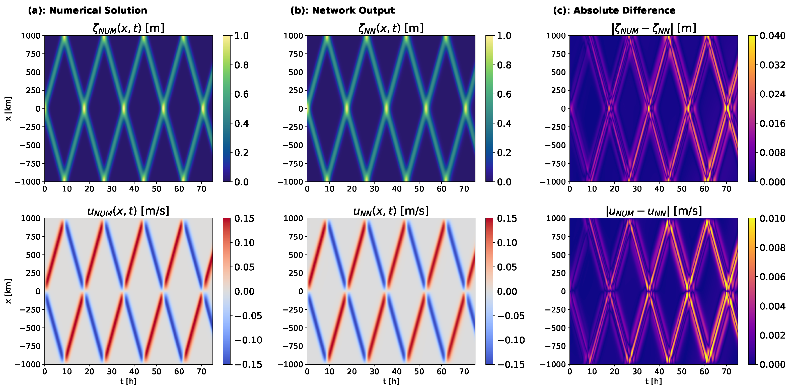
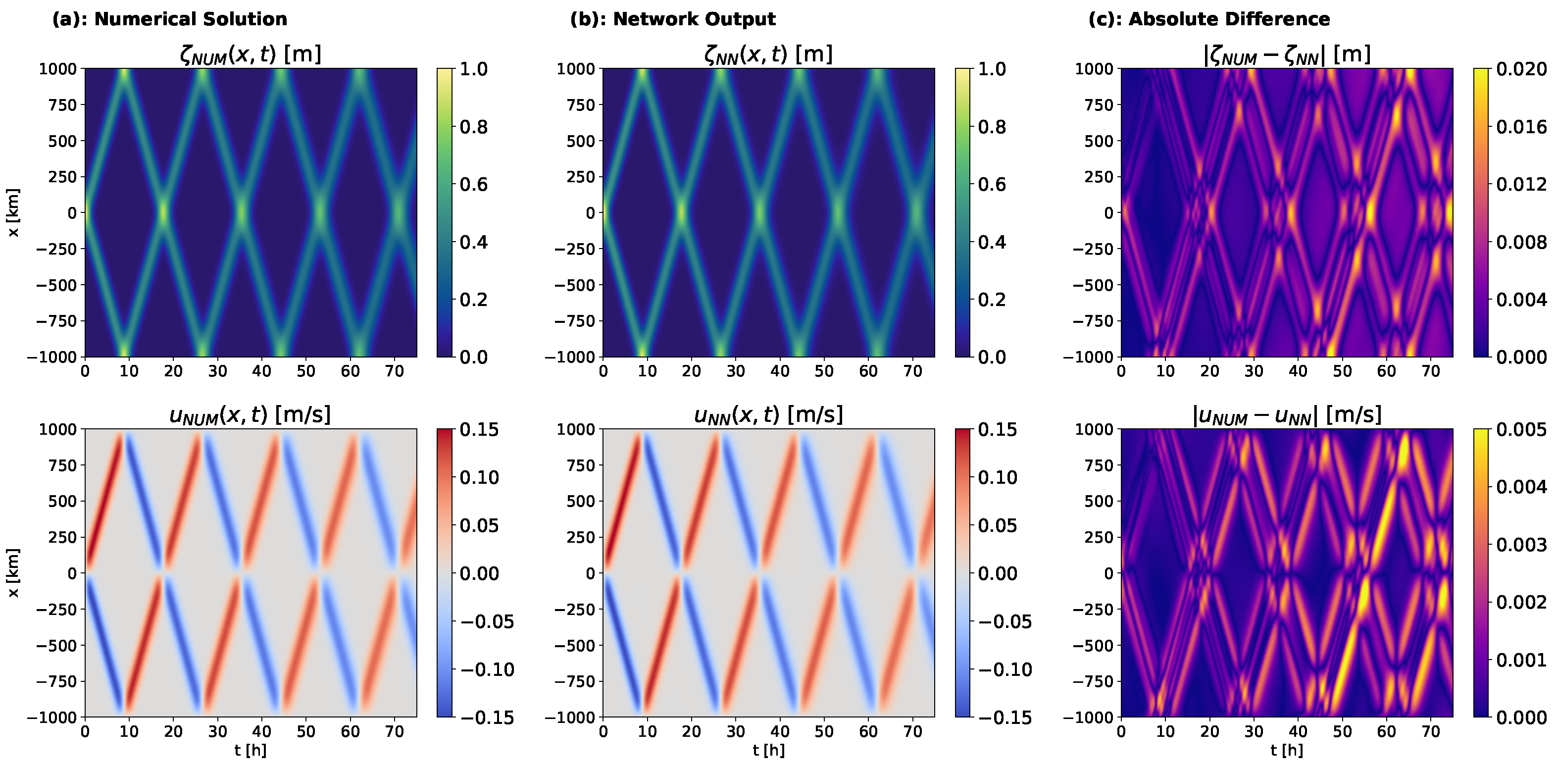
Using these default settings, we applied PINNs to solve two versions of the SWEs. In scenario A, waves propagate without the horizontal diffusion of velocity ($A_H=0$, Figure 6a), while in scenario B they slowly dissipate due to the dispersive PDE term ($A_H=5\times {10}^4{\mathrm{m}}^2{\mathrm{s}}^{-1}$, Figure 7a). In both scenarios, the initial Gaussian bell splits into to waves that reflect repeatedly from the domain boundaries. For both scenarios, training PINNs with our default settings yielded a PDE solution that closely resembled the numerical solution, with all wave reflections represented and errors 1–2 orders of magnitude smaller than the solutions (Figure 6b,c and Figure 7b,c). Errors tended to increase over time and were highest around the wave peaks. We quantified these errors using ${\mathcal{L}}_{\mathrm{NUM},2}$- and ${\mathcal{L}}_{\mathrm{NUM},\infty }$-norms (Equations (29)–(32)), averaging over five training runs with random initialization, which exhibited high consistency (

Table 3. Differences compared to the numerical reference solution for cases A ($A_H=0$) and B ($A_H=5\times {10}^4{\mathrm{m}}^2{\mathrm{s}}^{-1}$) for models trained on the PINNs loss function and models trained supervised (SUP) on the reference solution. Here, we set $N_{\mathrm{IC}},N_{\mathrm{BC}}=4\times {10}^4$, $N_{\mathrm{PDE}}=1\times {10}^5$ with a network size $4\times 100$ and using PCGrad https://github.com/WeiChengTseng/Pytorch-PCGrad (accessed on 15 August 2024).

Model	PINN-A	PINN-B	SUP-A	SUP-B
${\mathcal{L}}_{\mathrm{NUM},2}\left(\zeta \right)$ [%]	$3.15$	$2.15$	$0.30$	$0.26$
${\mathcal{L}}_{\mathrm{NUM},2}\left(u\right)$ [%]	$3.76$	$2.71$	$0.62$	$0.60$
${\mathcal{L}}_{\mathrm{NUM},\infty }\left(\zeta \right)$ [%]	$5.93$	$2.15$	$0.75$	$0.58$
${\mathcal{L}}_{\mathrm{NUM},\infty }\left(u\right)$ [%]	$10.22$	$4.02$	$2.86$	$3.04$
$t_{\mathrm{comp}}$ [h]	$64.32$	$64.38$	$25.46$	$33.11$

). Average errors ranged from 3 to 10% depending on the error metric and PDE variable, but were generally higher for horizontal velocity than for elevation.

These results show, to our knowledge for the first time, that PINNs can learn solutions to SWEs with closed boundaries. However, convergence for both scenarios required $>64$ h over ten thousand epochs on a single GPU. Clearly, this cost–accuracy trade-off is not competitive with conventional numerical methods which required, depending on resolution, from one minute to two hours on a single central processing unit (CPU). We therefore focused our subsequent experiments on understanding how the PINNs optimization process arrives at a PDE solution, and whether the specialized techniques proposed for training PINNs could produce an accurate solution more quickly.

3.2. Evolution of PDE Solution and Loss Terms During Training

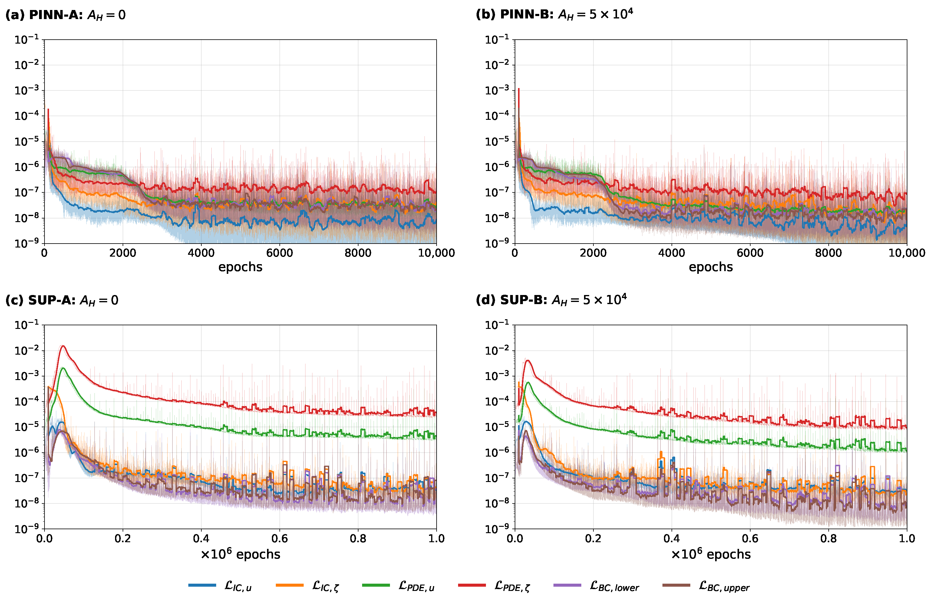
To investigate how PINNs converge to solutions of the SWEs, we tracked individual loss terms and differences from the reference solution over the optimization process (Figure 8a,b). A more detailed representation of the individual contributions to the PINNs loss function is given in Figure 9a,b, where the loss functions for the PDEs and initial conditions are shown separately for $\zeta$ and u, and for both individual boundary conditions for u as well. The relation between the changes in the difference to the reference solution and the PINNs loss can be used to determine how the physics-informed optimization contributes to higher accuracy.

In both cases, the differences between the reference solution ${\mathcal{L}}_{\mathrm{NUM},\zeta }$ and ${\mathcal{L}}_{\mathrm{NUM},u}$ decrease slowly for up to roughly 2000 epochs. Between 2000 and 4000 epochs, they rapidly decrease by between one and two orders of magnitude and finally continue to decrease steadily at a low rate (see Figure 8a,b). The period with the largest decline in the difference to the reference solution coincides with a steep decrease in the boundary condition loss ${\mathcal{L}}_{\mathrm{BC}}$, whereas the initial condition and PDE losses ${\mathcal{L}}_{\mathrm{IC}}$ and ${\mathcal{L}}_{\mathrm{PDE}}$ decrease more steadily. In contrast, the latter most strongly decrease within the initial 1000 epochs when the network approximation is still highly inaccurate.

This demonstrates that, to achieve fast convergence to accurate solutions, it is crucial to closely obey the no-outflow boundary conditions. This fast decline can also be seen in the momentum equation loss ${\mathcal{L}}_{\mathrm{PDE},u}$, but not in the continuity equation loss ${\mathcal{L}}_{\mathrm{PDE},\zeta }$ (see Figure 9a,b), which indicates a connection to the boundary conditions, for example, at the locations of reflection. The steady late training period from 4000 to $10,000$ epochs significantly improves the final model’s accuracy, but also more than doubles the amount of time required to obtain a feasible solution due to the low rate of decrease in the difference from the reference solution. Nonetheless, a reduction in the number of epochs may degrade the resulting solutions unacceptably. Overall, the difference compared to the reference solution is on the upper end of the estimated uncertainty range in the reference solution. Therefore, the network approximation can overall be said to have solved the PDE. For case B, the approximation shows even higher accuracy, which suggests that the model is adaptable to various physical settings.

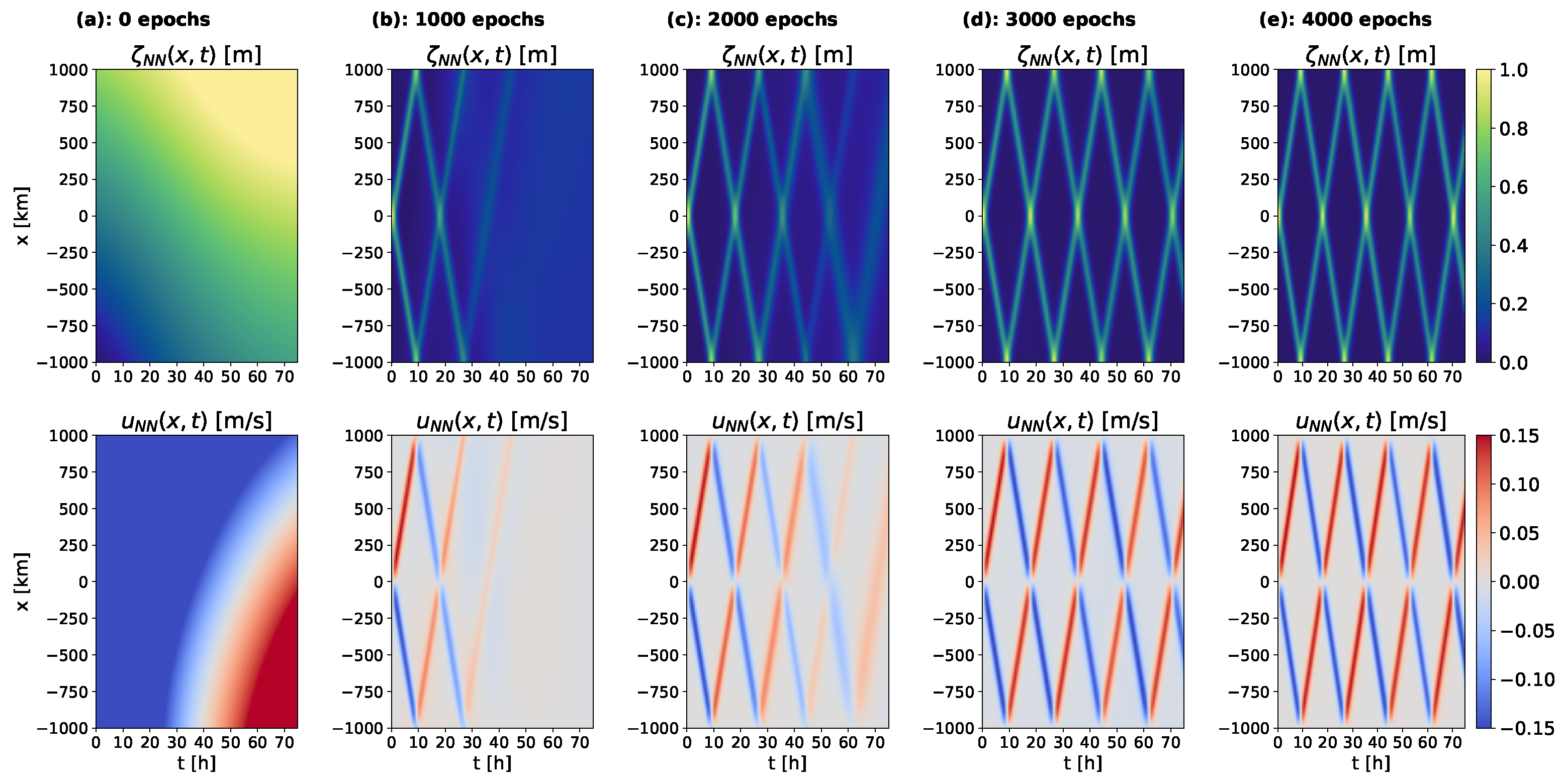
3.3. Evolution of the Network Approximation over Training

In an effort to analyze the training process and to identify the factors impeding fast convergence, we compared the network output for $\zeta$ and u, and the spatiotemporal distribution of the PDE residuals $f_{\zeta }$ and $f_u$ throughout the model optimization. The evolution of the network output and PDE residuals for case A are shown in Figure 10 and Figure 11, respectively, over the first 4000 epochs of training, which is consistent with other model experiments, including case B.

The change in the network approximations for $\zeta$ and u (see Figure 10) illustrates the step-wise learning process of the PINN-based model over the time interval. At each training step, the output only shows a further wave propagation after the previous propagation and reflections have been learned. This process resembles a wave propagation over time or a step-wise integration of the wave signal. Despite the minimization of the PDE loss over the entire domain at all gradient steps, the solution is learned sequentially in time, approaching the reference solution from earlier to later states.

This sequential learning of the solution is in accordance with the different rates of decrease in the difference to the reference solution over the optimization in the training curve (see Figure 8a). Over the initial 2000 epochs, the network approximation strongly deviates from the reference solution in a large part of the domain. Between 2000 and 3000 epochs, the network completely learns the pattern of wave propagation, which causes a rapid decrease in the differences to the reference solution. In the subsequent epochs, the network makes small adjustments over the entire domain, leading to the low rate of decrease in the differences to the reference solution between 4000 and 10,000 epochs.

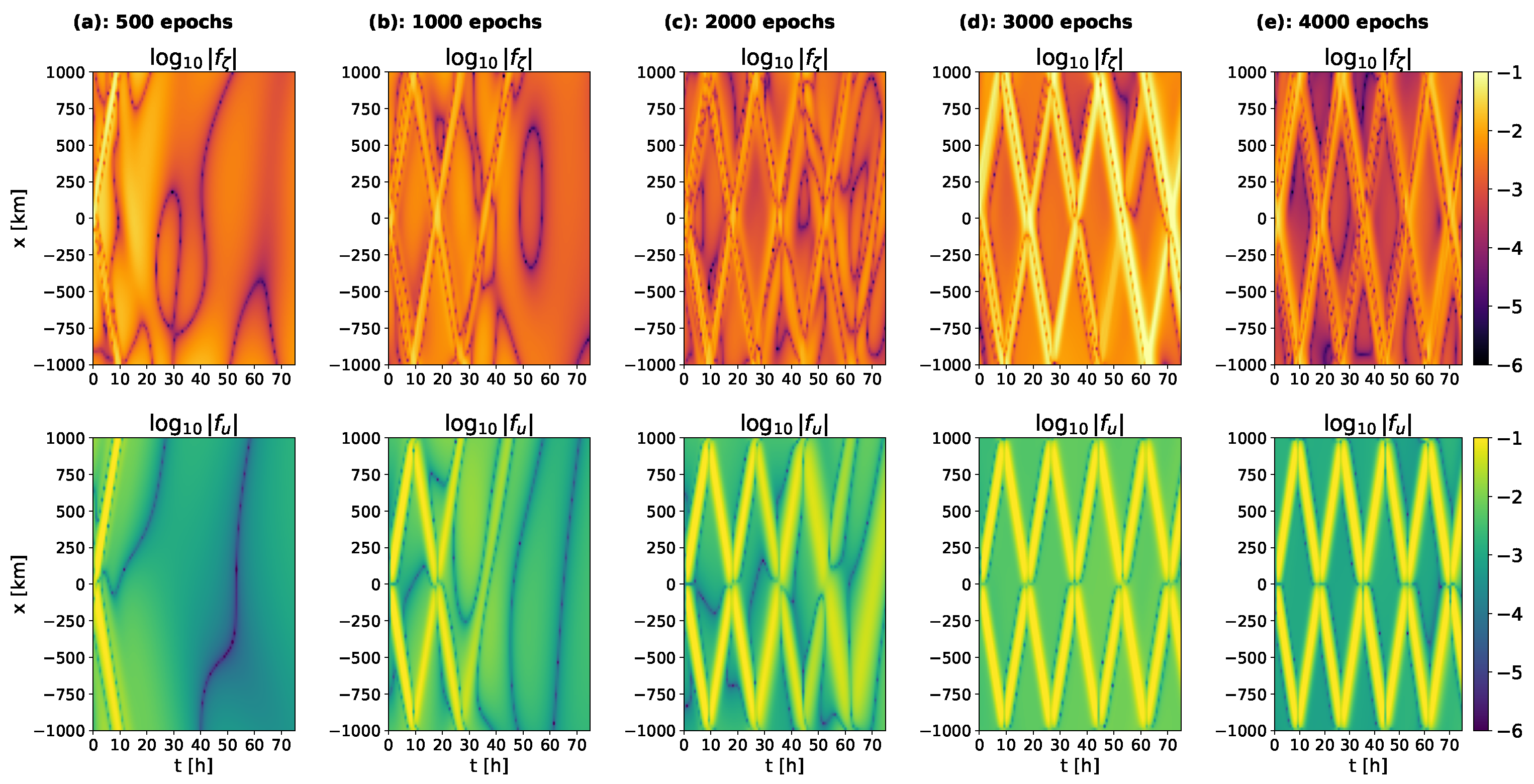
Comparing the changes in the continuity and momentum equation (see Figure 11) residuals over training, the sequential learning of the wave propagation is apparent in both residuals. While the areas of undisturbed sea level show a steady decrease in the residuals over the first 4000 epochs, they increase by several orders of magnitude in the areas of wave propagation. This mismatch between the changes in the PDE residuals and the difference from the reference solution show that low PDE residuals do not guarantee accurate solutions, but accurate solutions do not necessarily lead to low PDE residuals.

These findings suggest that both the initial learning of the wave propagation and the slow convergence to the reference solution in the later training period contribute to long training times. The sequential learning of the individual reflections underlines the importance of the accurate representation of the boundary conditions to the ability to model all wave reflections. It is also consistent with the previously noted coincidence between the decrease in the differences from the reference solution and boundary condition losses.

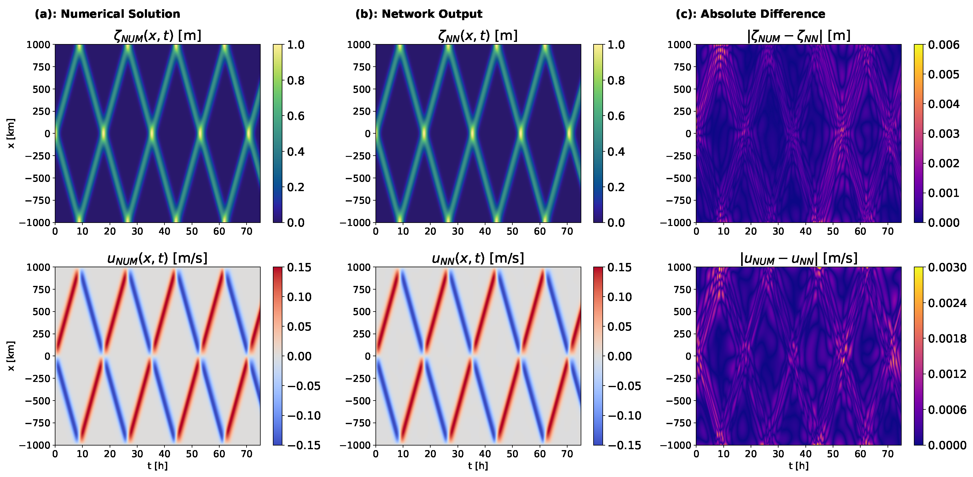
3.4. Supervised Training on the Reference Solution

To evaluate the possible limitations of the approximation ability of the neural architecture regarding the quality and speed of convergence, we trained neural networks to solve cases A and B to determine whether the network is able to learn the reference solution more accurately when trained directly on the numerical solution with a supervised least squares loss. As in the previous experiments, we show the numerical reference solution, the network approximation after training, and their absolute difference for both $\zeta$ and u in Figure 12 and Figure 13, with the respective differences in the ${\mathcal{L}}_{\mathrm{NUM},2}$- and ${\mathcal{L}}_{\mathrm{NUM},\infty }$-norms shown in the last two columns of Table 3.

When trained directly on the reference solution, the network approximation’s difference from the reference solution is, below $0.5$% and 1% in the ${\mathcal{L}}_{\mathrm{NUM},2}$-norm, and below 1% and roughly 3% in the ${\mathcal{L}}_{\mathrm{NUM},\infty }$-norm for $\zeta$ and u, respectively, in both test cases (see Table 3). The absolute differences compared to the reference solution do not show an increase over the time interval, as they did for the physics-informed optimization (see Figure 12c and Figure 13c). In comparison to the PINN-based model, the training curves show a more gradual decrease in all loss terms over the entire training period, except from some initial fluctuations in the initial and boundary condition losses (see Figure 8c,d and Figure 9c,d). During this initial training period, the PDE losses rapidly increase, but then continue to steadily decrease. This initial peak may be due to the absence of physical constraints in this case, allowing for physically inconsistent solutions if they lead to a better match with the reference solution. While the initial and boundary condition losses are comparable for both training modes, training on the reference solution leads to higher PDE losses in the final network output by approximately two orders of magnitude.

These results suggest that the approximation capability is not a limiting factor for the model accuracy and does not impede fast convergence. Rather, the error accumulation over time and the slow sequential learning of the wave propagation in the PINN-based model may be caused by optimization problems originating from the PDE loss function. This is also indicated by the mismatch between accurate solutions and low PDE residuals that occurs both when training on the reference solution and when using the physics-informed loss. Another possible source of the differences in the two training modes is uncertainty in the reference solution itself.

3.5. Sensitivity Study

We additionally assessed how the accuracy of the PINN-based solution could depend on estimation errors arising from the finite set of control points as well as the network architecture. To this end, we performed sensitivity experiments on the total number of control points $N_{\mathrm{IC}}$, $N_{\mathrm{BC}}$ and $N_{\mathrm{PDE}}$ per epoch, and on the network width and depth (i.e., the number of layers and number of activations in each layer). The accuracy reached in two additional experiments, with one half and a quarter of the control points, was compared to the default experiment of test case B in

Table 4. Differences compared to the numerical reference solution for different numbers of collocation points for $A_H=5\times {10}^4$m²/s. All other training parameters are equal to Table 3.

${\mathit{N}}_{\mathbf{IC}}$, ${\mathit{N}}_{\mathbf{BC}}$	$1\times {10}^4$	$2\times {10}^4$	$4\times {10}^4$
${\mathit{N}}_{\mathbf{PDE}}$	$\mathbf{2}.\mathbf{5}\times {\mathbf{10}}^{\mathbf{4}}$	$\mathbf{5}\times {\mathbf{10}}^{\mathbf{4}}$	$\mathbf{1}\times {\mathbf{10}}^{\mathbf{5}}$
${\mathcal{L}}_{\mathrm{NUM},2}\left(\zeta \right)$ [%]	$1.95$	$1.98$	$2.15$
${\mathcal{L}}_{\mathrm{NUM},2}\left(u\right)$ [%]	$2.50$	$2.53$	$2.71$
${\mathcal{L}}_{\mathrm{NUM},\infty }\left(\zeta \right)$ [%]	$1.91$	$1.91$	$2.15$
${\mathcal{L}}_{\mathrm{NUM},\infty }\left(u\right)$ [%]	$3.34$	$3.37$	$4.02$
$t_{\mathrm{comp}}$ [h]	$27.57$	$37.40$	$64.38$

. Similarly, for two smaller network sizes with 2 and 3 layers, with 30 and 50 activations per layer, respectively, the comparison with the default network architecture is shown in

Table 5. Differences compared to the numerical reference solution for different network sizes with $N_{\mathrm{IC}},N_{\mathrm{BC}}=1\times {10}^4$, $N_{\mathrm{PDE}}=2.5\times {10}^4$ for $A_H=5\times {10}^4$m²/s. All other training parameters are as in Table 3.

Network Size	$2\times 30$	$3\times 50$	$4\times 100$
${\mathcal{L}}_{\mathrm{NUM},2}\left(\zeta \right)$ [%]	$65.83$	$47.65$	$1.95$
${\mathcal{L}}_{\mathrm{NUM},2}\left(u\right)$ [%]	$82.68$	$59.90$	$2.50$
${\mathcal{L}}_{\mathrm{NUM},\infty }\left(\zeta \right)$ [%]	$64.57$	$54.33$	$1.91$
${\mathcal{L}}_{\mathrm{NUM},\infty }\left(u\right)$ [%]	$84.83$	$70.71$	$3.34$
$t_{\mathrm{comp}}$ [h]	$24.32$	$25.57$	$27.57$

. In these experiments, we set the number of sampling points to the lowest setting.

For all three experiments with variable numbers of sampling points, there is close to no difference in accuracy and the differences compared to the reference solution are consistently between 2 and 4% in the ${\mathcal{L}}_{\mathrm{NUM},2}$- and ${\mathcal{L}}_{\mathrm{NUM},\infty }$-norms (see Table 4). This means that there is no considerable influence of estimation errors that would lead to the over-fitting of too-small sample sizes. Instead, when using far fewer control points, an equal accuracy can be maintained.

In contrast to this, the observed accuracy strongly depends on the network size. For both smaller network sizes, the network approximations are inaccurate, with differences compared to the reference solution of above 47% and 64% for $\zeta$ and above 59% and 82% for u in both norms. Hence, network sizes much smaller than the one used in the default experiment are not feasible for this task (see Table 5). While even larger network sizes might improve accuracy, we did not consider them here for two reasons. Firstly, we reached the limit of the memory and run time on a single GPU. Secondly, supervised training on the reference solution showed an even higher accuracy compared to the PINN solutions when using the same network architecture. For this reason, we conclude that network size was not a significant limitation for the scenarios we studied.

Together, the results of training on the reference solution and the sensitivity experiments indicate that neither approximation nor estimation errors pose a limitation to the quality and speed of convergence. As a consequence, in subsequent experiments, we focused on improving the optimization with specialized training modes.

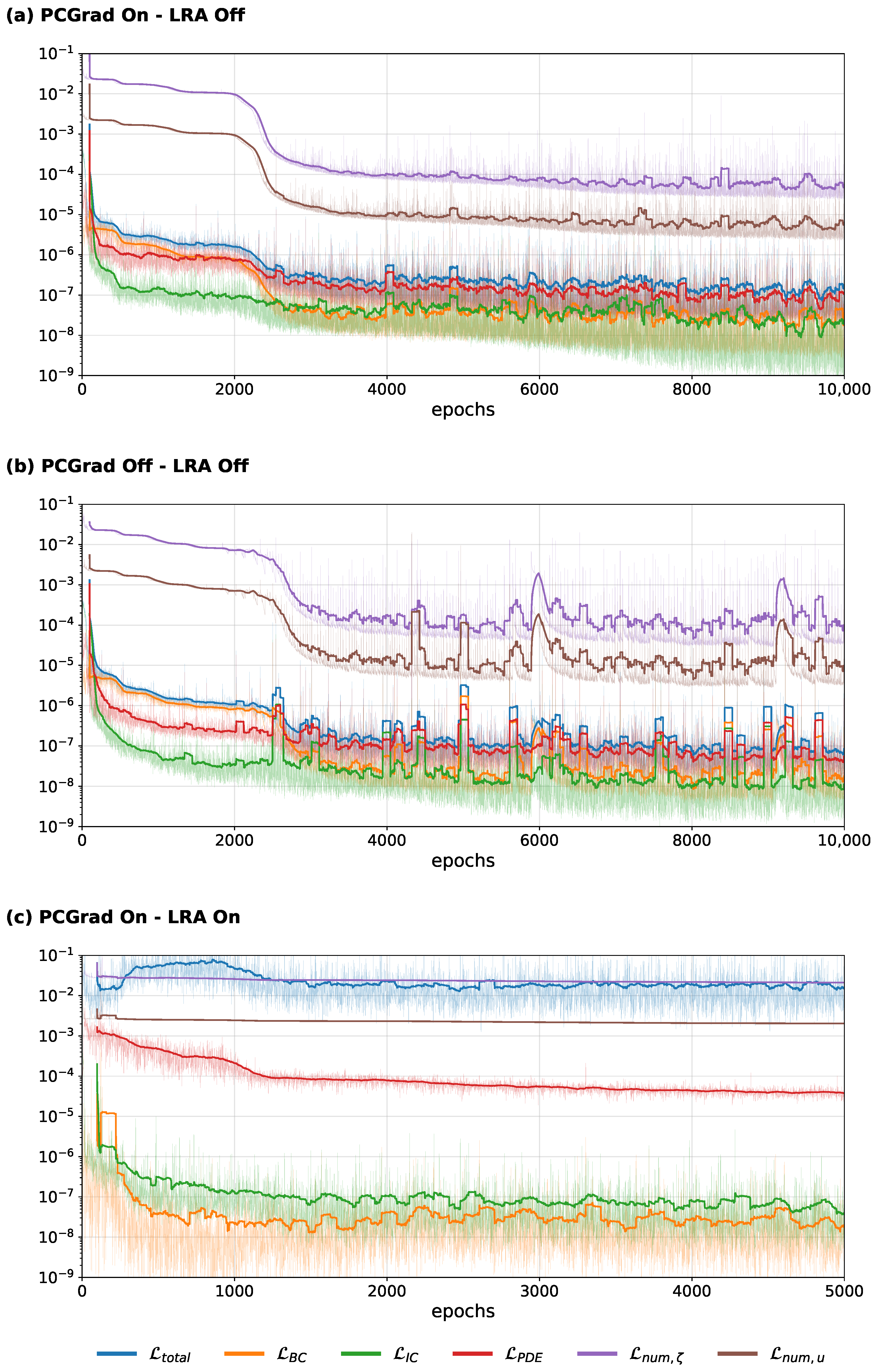
3.6. Specialized Training Modes

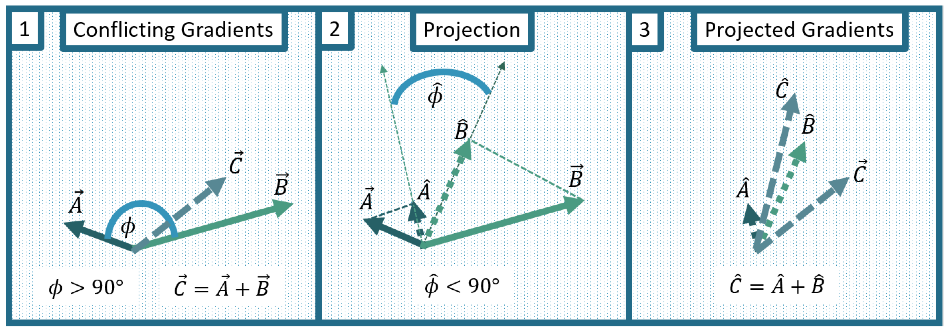
With the aim of improving the speed and quality of convergence, we tested two specialized training modes: the projection of conflicting gradients (PCGrad) and an adaption of the loss weights $w_{\mathrm{PDE}}$, $w_{\mathrm{BC}}$ and $w_{\mathrm{IC}}$ over training, called learning rate annealing (LRA). While we had already applied PCGrad in the default setup, we here compare the optimization properties with and without this method. We compared three different experiments for case B: the first using neither of the two methods, the second only using PCGrad, and the third using both PCGrad and LRA. The differences compared to the reference solution are shown in

Table 6. Differences compared to the numerical reference solution for training settings with and without the use of PCGrad and Learning Rate Annealing with $A_H=5\times {10}^4$ m²/s. All other training parameters are equal to Table 3.

PCGrad	Off	On	On
LRA	Off	Off	On
${\mathcal{L}}_{\mathrm{NUM},2}\left(\zeta \right)$ [%]	$2.85$	$2.15$	$72.87$
${\mathcal{L}}_{\mathrm{NUM},2}\left(u\right)$ [%]	$3.59$	$2.71$	$91.14$
${\mathcal{L}}_{\mathrm{NUM},\infty }\left(\zeta \right)$ [%]	$2.68$	$2.15$	$74.50$
${\mathcal{L}}_{\mathrm{NUM},\infty }\left(u\right)$ [%]	$4.51$	$4.02$	$90.48$
$t_{\mathrm{comp}}$ [h]	$63.58$	$64.38$	$59.34$

and the respective training curves are shown in Figure 14.

The use of PCGrad leads to a small but consistent improvement in the achieved accuracy, of approximately 0.5–1% in the ${\mathcal{L}}_{\mathrm{NUM},2}$- and ${\mathcal{L}}_{\mathrm{NUM},\infty }$-norms (see Table 6). Moreover, when comparing the evolution of the difference to the reference solution as well as the individual parts of the PINNs objective function (see Figure 14a,b), the experiment without PCGrad shows higher-amplitude oscillations, both in the running mean (solid line) and in the loss per epoch (shaded line). These high-frequency oscillations not only locally increase the difference from the reference solution, but also contribute to instabilities in the training. Specifically, at approximately 6000 and 9200 epochs, increases of about two orders of magnitude in the differences from the reference solution can be seen for the experiment without PCGrad (see Figure 14b). The experiment using PCGrad does not show any sudden increases in the differences from the reference solution and generally contains lower oscillations with a more consistent decrease. This may improve the training efficiency and, ultimately, the accuracy. Nevertheless, no significant speedup in convergence could be achieved.

To assess if LRA could lead to an improvement in optimization, we tested it both in combination with PCGrad and on its own. As the results were equal in both cases, we here only report those obtained in combination with PCGrad. For this case, the differences compared to the reference solution remained above 70% for $\zeta$ and above 90% for u (see Table 6). Considering the minimization of the individual parts of the composite objective function (see Figure 14c), there seems to be an imbalance in the consideration of the PDE loss term compared to the initial and boundary conditions. While the latter decrease rapidly at the beginning of training, the PDE loss only decreases at a very low pace throughout the optimization. This indicates that LRA fails to equally optimize the individual learning tasks and therefore impedes accurate solutions. Due to the additional computation time caused by the LRA algorithm, the amount of epochs was reduced to 5000 for a comparable cost of training.

Despite small improvements in the stability and accuracy of training when using the PCGrad method, none of the two methods led to a sufficient speedup that would make the cost of training feasible. A comparison of the results for both methods suggests that, in this particular case, the occurrence of conflicting gradients from individual learning tasks was more relevant than the respective weights.

3.7. Hard Constraints on Initial and Boundary Conditions

Some of the previous results indicated that, for the PINN-based model, the sequential learning of the wave propagation, and particularly learning the reflections, contributes to the slow convergence (see Figure 8a,b and Figure 10). Obeying the no-outflow boundary conditions was shown to be important for an accurate representation of the wave propagation, as the difference to the reference solution decreases rapidly with decreasing boundary condition losses (see Figure 8 and Figure 9a,b). To address this, we modified the network architecture by applying transition functions so that the network output always satisfies the boundary conditions, and in some cases also the initial conditions, regardless of the network parameters. The aim was to speed up convergence by reducing the number of learning tasks and facilitating the learning of the wave propagation and reflections. Furthermore, this could prevent local violations of the boundary conditions that could lead to inaccurate solutions. The differences between the network approximation and the reference solution for all three tested transition functions ${\mathcal{T}}_1$, ${\mathcal{T}}_2$ and ${\mathcal{T}}_3$ are shown in

Table 7. Differences compared to the numerical reference solution for architectures with all three transition functions and the default case for comparison with $A_H=5\times {10}^4$ m²/s. All other training parameters are equal to Table 3.

Transition Function	None	${\mathcal{T}}_1$	${\mathcal{T}}_2$	${\mathcal{T}}_3$
${\mathcal{L}}_{\mathrm{NUM},2}\left(\zeta \right)$ [%]	$2.15$	$55.28$	$54.33$	$57.90$
${\mathcal{L}}_{\mathrm{NUM},2}\left(u\right)$ [%]	$2.71$	$69.45$	$68.10$	$72.59$
${\mathcal{L}}_{\mathrm{NUM},\infty }\left(\zeta \right)$ [%]	$2.15$	$57.20$	$57.36$	$59.27$
${\mathcal{L}}_{\mathrm{NUM},\infty }\left(u\right)$ [%]	$4.02$	$72.07$	$73.10$	$73.08$
$t_{\mathrm{comp}}$ [h]	$64.38$	$56.00$	$58.46$	$58.21$

and the respective training curves are shown in Figure 15.

As a first test, we applied the transition function ${\mathcal{T}}_1$ to only constrain both boundary conditions. Despite reducing the amount of learning tasks and accurately representing the boundary conditions, the network approximation did not achieve any differences compared to the reference solution below 50% (see Table 7). The change in the PDE and initial condition losses over training shows that the optimization failed to minimize both equally. While the initial condition loss rapidly decreased at the beginning of training, the PDE loss converged above a high threshold, thereby preventing accurate solutions (see Figure 15b). To reduce the amount of learning tasks even further and additionally satisfy the initial condition implicitly, we tested two further transition functions ${\mathcal{T}}_2$ and ${\mathcal{T}}_3$. Still, the network optimization failed to sufficiently decrease the PDE residuals and equally obstructed the convergence to accurate solutions (see Figure 15c,d). The differences compared to the reference solution here also remained above 50%. Accordingly, no improvement in the quality or speed of convergence was reached.

4. Discussion

4.1. Main Obstacles to Accuracy and Efficiency

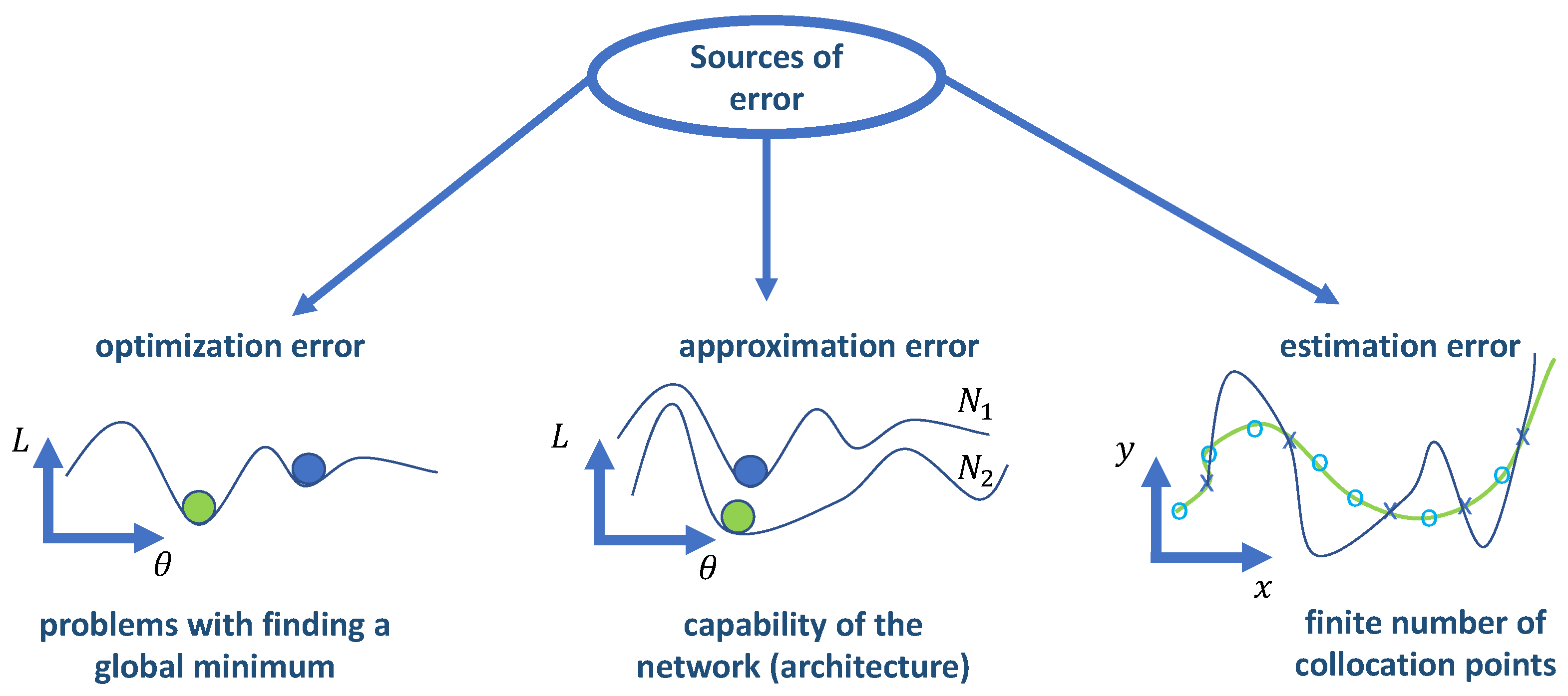
We demonstrated that, although PINNs can learn wave reflection scenarios based on the shallow water equations (SWE), this comes at the cost of unfeasible training times. Our experiments suggest that the primary limitations in quality and convergence speed are not due to the network architecture’s approximation capability or estimation errors (see Table 3, Table 4 and Table 5). Instead, we observed systematic characteristics of the optimization process that limit the efficiency of PINNs in this task and may extend to other applications.

One key factor limiting accuracy is the rapid accumulation of errors over the time domain, reflected in the increase in the absolute differences between the reference solution and the PINN-based model’s approximation (see Figure 6c and Figure 7c). This error accumulation does not occur when using supervised training on the reference solution, suggesting that it stems from the physics-informed optimization process rather than the network architecture’s approximation capacity.

Regarding convergence speed, the main obstacle is the sequential learning of wave propagation, which is hindered by the challenge of learning wave reflections at the boundaries (see Figure 10). Attempts to mitigate these limitations, such as adjustments to the optimization strategy, yielded only marginal improvements. In the following sections, we elaborate on these two aspects and discuss them in the context of the existing research.

4.2. Accumulation of Errors and Locality

To illustrate how errors accumulate over time in the PINN approximation, despite the continuous representation of the solution, we provide an upper bound for the absolute difference between the approximate solution $\widehat{f}(x,t)$ and the exact solution $f(x,t)$. In this idealized setting, we assume that both $\widehat{f}(x,t)$ and $f(x,t)$ are continuously evaluated, with $\widehat{f}(x,t)$ perfectly matching the true boundary conditions. The absolute difference is then bounded by the difference in the initial states $\widehat{f}(x,0)$ and $f(x,0)$, plus the time-integrated absolute difference between their time derivatives, as shown in Equation (33).

This time-integrated difference can be expressed as the product of time t and the expected value ${\mathbb{E}}_{t^{\prime }\sim \mathbb{U}(0,t)}$. When the initial conditions are perfectly represented, i.e., $|\widehat{f}(x,0)-f(x,0)|=0$, the upper bound reduces to a term that scales linearly with time. Thus, even with perfect initial conditions and a continuous representation of PDE residuals, small differences in the derivatives may accumulate over time. While the PINN optimization does not directly minimize the difference in the time derivatives, but rather a sum of derivatives expressed by the PDEs, we assume for this idealized comparison that low-PDE residuals would also lead to low differences in the time derivatives themselves.

Although automatic differentiation and the continuous solution representation offer advantages over traditional discrete numerical integration by reducing step-wise errors, these small discrepancies in the derivatives can grow significantly over long intervals. This is exacerbated by the discrete evaluation of all loss terms, including PDE residuals, and the imperfect representation of the initial and boundary conditions.

$$\begin{array}{c}\hfill |\widehat{f}(x,t)-f(x,t)|=\left|\right[\widehat{f}(x,t)-\widehat{f}(x,0)]+\widehat{f}(x,0)-([f(x,t)-f(x,0)]+f(x,0)\left)\right|\\ \hfill =\left|\right[\widehat{f}(x,t)-\widehat{f}(x,0)]-[f(x,t)-f(x,0)]+[\widehat{f}(x,0)-f(x,0)]|\\ \hfill \le |\widehat{f}(x,0)-f(x,0)|+\left|\right[\widehat{f}(x,t)-f(x,t)]+[\widehat{f}(x,0)-f(x,0)\left]\right|\\ \hfill =|\widehat{f}(x,0)-f(x,0)|+|{\int }_{t^{\prime }=0}^{t^{\prime }=t}{\displaystyle \frac{\partial \widehat{f}(x,t^{\prime })}{\partial t}}-{\displaystyle \frac{\partial f(x,t^{\prime })}{\partial t}}d{t}^{\prime }|\\ \hfill \le |\widehat{f}(x,0)-f(x,0)|+{\int }_{t^{\prime }=0}^{t^{\prime }=t}|{\displaystyle \frac{\partial \widehat{f}(x,t^{\prime })}{\partial t}}-{\displaystyle \frac{\partial f(x,t^{\prime })}{\partial t}}|d{t}^{\prime }\\ \hfill =|\widehat{f}(x,0)-f(x,0)|+t·{\mathbb{E}}_{t^{\prime }\sim \mathbb{U}(0,t)}|{\displaystyle \frac{\partial \widehat{f}(x,t^{\prime })}{\partial t}}-{\displaystyle \frac{\partial f(x,t^{\prime })}{\partial t}}|\end{array}$$

(33)

Firstly, PDE residuals in PINN optimization are evaluated at a finite number of points rather than continuously, which can lead to faster error accumulation in unsampled regions of the domain where larger PDE violations may go undetected. Secondly, errors in the initial and boundary conditions propagate over time. Since the unique solution of the PDEs depends on these conditions, deviations from them allow the solution to diverge from the true solution without increasing the PDE violation.

This reliance on the accuracy of earlier states has been linked to a lack of consideration for the causal structure inherent to physical systems [29]. This stems from the evaluation of PDE residuals at point locations, which only reflect local violations at the specified time, without accounting for errors carried forward from previous states. In the absence of supervised information inside the domain, this will increase error accumulation over time. Combined, the accumulation of PDE violations over time, inaccuracies in initial and boundary conditions, and the locality of the residual evaluation present significant challenges to achieving optimal accuracy in the PINN optimization process. This is demonstrated by the increase in absolute differences over time in our experiments (Figure 6c and Figure 7c).

4.3. Sequential Learning

In our experiments, the evolution of the PINN approximation during optimization shows that, for the considered test cases, the PINNs learn an accurate representation of the system states sequentially over time. This means that PINN optimization requires an accurate representation of earlier states before later states can be captured (see Figure 10). This sequential learning may be tied to the propagation hypothesis and propagation failure [32] and the lack of physical causality [29] described in previous work. In the context of PINNs, supervised information about the true system state is typically confined to the initial and boundary conditions at the edges of the time interval. This limitation does not apply to scenarios where additional data are provided across the domain, such as during interpolation or data assimilation applications [3,92,93,94]. Within the unsupervised regions, the accuracy of the solution depends on the propagation of information from the initial and boundary conditions through the optimization of the PDE residuals [29,32]. In this context, accurate solutions are generally expected to propagate from supervised to unsupervised regions, which, while sequential in time for our case, could differ in other scenarios.

In our experiments, reflections were only learned once the wave propagation in the learned solution reached the boundary, leading to a conflict between the wave propagation and the boundary conditions. A wave propagation beyond the boundary does not increase the PDE loss, as it satisfies the PDE under open boundary conditions. As a result, the physics-informed training adjusts the learned solution to reconcile both the PDEs and the closed boundary conditions only after such a conflict arises. This reliance on initial and boundary condition propagation can be explained theoretically by the properties of the initial-boundary value problems. Without specified initial and boundary conditions, no unique solution exists, but rather a family of solutions that satisfies the PDEs. This means that PDE residuals may remain low even for inaccurate solutions, provided they satisfy the PDEs within the domain.

A clear example of this is when wave heights and velocities drop to zero within a short time interval. Early in training, we observed that the network approximation (Figure 10b) approaches zero in the second half of the time interval, corresponding to lower PDE residuals (Figure 11b), despite the solution being closer to the reference solution at the start of the interval. Conversely, an accurate solution can have high PDE residuals if earlier states are inaccurate or if small-scale variability causes PDE violations without significantly reducing accuracy. This may explain the higher PDE residuals that were obtained for the accurate solutions when training on the reference solution (see Figure 9c,d).

The dependence on earlier states has several implications for optimization. First, each gradient step is limited in how much it can improve the solution’s propagation based on the current approximation. Consequently, the optimization requires many training steps to propagate information through the domain. Second, localized boundary conditions or PDE violations with low total loss contributions can lead to the dissipation of the solution within a small time interval. This indicates that intermittent increases in the total loss function are essential for attaining the global optimum and achieving an accurate approximation. Furthermore, this implies that the second-order LBFGS optimizers rapidly converged to local minima, thereby preserving inaccurate solutions. This property of PINN optimization, where second-order methods converge to saddle points for non-convex loss functions due to the missing consideration of negative curvature, has been noted in previous studies, with first-order methods often showing superior results by avoiding such convergence [95].

Recent advancements aim to address some of these challenges with various strategies. To mitigate the lack of causality between different time states, a causality parameter was introduced into the PDE loss formulation to control the weighting of PDE residuals at each location, enforcing the minimization of earlier residuals before moving to later states [29]. Additionally, evolutionary sampling methods were developed to prioritize sampling in causally relevant regions of the domain [32]. There has also been a shift from using the $L_2$-norm for the PDE loss to the $L_{\infty }$-norm, which can better account for the high local violations that could lead to spurious solutions [56]. Hybrid PINN methods that incorporate discretized numerical approximations have also been explored, speeding up convergence by linking neighboring locations within the domain [34,35,36]. Another promising branch of PINN development towards additional constraints is network architectures incorporating Hamiltonian mechanics [96,97,98,99], which have recently been extended from ordinary to partial differential equations [97]. With respect to modeling ocean waves, specialized optimization algorithms such as the nature-inspired water wave optimization algorithm [100] may also improve the accuracy and efficiency of PINN optimization.

4.4. Limitations

Our results should be viewed in the context of several limitations. First, it is challenging to assess the efficiency of training PINNs, as well as the utility and generality of specialized training approaches, across a wide variety of problems. This study provides a detailed analysis of a very specific scenario, and the results may not be directly applicable to other contexts. Furthermore, the range of optimization methods, sampling strategies, and network architectures considered was limited to maintain computational feasibility. The exploration of further hyperparameter configurations, including the choice of scaling parameters, may offer further potential for increasing efficiency. In addition, we limited the training time to 72 h using a GPU due to the practical requirements of real-world applications such as storm surge and tsunami prediction, where both accuracy and speed are critical. In these scenarios, with lead times ranging from only a few hours to a few days, the time available for computation is also limited to a few hours. Despite these limitations, our results provide valuable insights that can inform the future development of PINNs, particularly for geophysical fluid dynamics and coastal applications.

5. Conclusions

In this study, we demonstrated that physics-informed neural networks can successfully learn wave reflection scenarios based on the 1D SWE, which are relevant for geophysical fluid dynamics in coastal applications. However, optimization challenges arising from the physics-informed loss function limit both the speed and quality of convergence. These limitations are primarily due to the accumulation of errors over time and the sequential learning of the solution, both of which depend on the accuracy of earlier system states [29,32]. Since existing PINN-specific techniques did not yield significant improvements in training efficiency, we propose that this problem may serve as a valuable test case for future advancements in physics-informed machine learning.

To expand this application to operational forecasting systems aiming to predicting significant or maximum wave heights during storm surges or tsunamis, several development steps remain. First, PINN models must be extended to two-dimensional domains with complex features such as areas with varying topography, coastlines, and estuaries. These models would also require additional boundary conditions to account for open boundaries, tidal influences, and wind forcing. While previous attempts have explored replacing SWE-based flood models with PINNs using simplified wave equations [101], SWE-based PINNs still need to prove their suitability for such applications.

Furthermore, the current training approach is limited to specific initial conditions, meaning that each new prediction would require retraining the model. Ongoing work on generalizing neural networks for initial and boundary conditions, such as the deep operator network (DeepONet) [102] and multiple-input operator network (MIONet) [103], alongside proposed extensions for physics-informed training [104,105,106,107], could resolve this issue. By eliminating the need for repeated training, PINNs could enable faster predictions for new conditions.

In the broader context of PINN development, this work highlights the need for specialized training methods that address potential failure modes and slow convergence. Recent advances, including evolutionary sampling [32], hybrid PINNs with discretized difference approximations [34,35,36], and causality-respecting PINNs [29], show promise in improving the efficiency of PINNs. The development of efficient and scalable training methods will be crucial to making PINNs competitive with traditional numerical methods.

References

1. Karniadakis, G.E.; Kevrekidis, I.G.; Lu, L.; Perdikaris, P.; Wang, S.; Yang, L. Physics-informed machine learning. Nat. Rev. Phys. 2021, 3, 422–440. [Google Scholar] [CrossRef]
2. Markidis, S. The Old and the New: Can Physics-Informed Deep-Learning Replace Traditional Linear Solvers? Front. Big Data 2021, 4, 669097. [Google Scholar] [CrossRef] [PubMed]
3. Raissi, M.; Yazdani, A.; Karniadakis, G.E. Hidden fluid mechanics: Learning velocity and pressure fields from flow visualizations. Science 2020, 367, 1026–1030. [Google Scholar] [CrossRef] [PubMed]
4. Wandel, N.; Weinmann, M.; Klein, R. Teaching the incompressible Navier–Stokes equations to fast neural surrogate models in three dimensions. Phys. Fluids 2021, 33, 047117. [Google Scholar] [CrossRef]
5. Cai, S.; Wang, Z.; Wang, S.; Perdikaris, P.; Karniadakis, G.E. Physics-Informed Neural Networks for Heat Transfer Problems. J. Heat Transf. 2021, 143, 060801. [Google Scholar] [CrossRef]
6. Arthurs, C.J.; King, A.P. Active training of physics-informed neural networks to aggregate and interpolate parametric solutions to the Navier-Stokes equations. J. Comput. Phys. 2021, 438, 110364. [Google Scholar] [CrossRef]
7. Jin, X.; Cai, S.; Li, H.; Karniadakis, G.E. NSFnets (Navier-Stokes flow nets): Physics-informed neural networks for the incompressible Navier-Stokes equations. J. Comput. Phys. 2021, 426, 109951. [Google Scholar] [CrossRef]
8. Muralidhar, N.; Bu, J.; Cao, Z.; He, L.; Ramakrishnan, N.; Tafti, D.; Karpatne, A. Physics-Guided Deep Learning for Drag Force Prediction in Dense Fluid-Particulate Systems. Big Data 2020, 8, 431–449. [Google Scholar] [CrossRef] [PubMed]
9. He, Q.; Tartakovsky, A.M. Physics-Informed Neural Network Method for Forward and Backward Advection-Dispersion Equations. Water Resour. Res. 2021, 57, e2020WR029479. [Google Scholar] [CrossRef]
10. Almajid, M.M.; Abu-Al-Saud, M.O. Prediction of porous media fluid flow using physics informed neural networks. J. Pet. Sci. Eng. 2022, 208, 109205. [Google Scholar] [CrossRef]
11. Kissas, G.; Yang, Y.; Hwuang, E.; Witschey, W.R.; Detre, J.A.; Perdikaris, P. Machine learning in cardiovascular flows modeling: Predicting arterial blood pressure from non-invasive 4D flow MRI data using physics-informed neural networks. Comput. Methods Appl. Mech. Eng. 2020, 358, 112623. [Google Scholar] [CrossRef]
12. Tartakovsky, A.M.; Marrero, C.O.; Perdikaris, P.; Tartakovsky, G.D.; Barajas-Solano, D. Physics-Informed Deep Neural Networks for Learning Parameters and Constitutive Relationships in Subsurface Flow Problems. Water Resour. Res. 2020, 56, e2019WR026731. [Google Scholar] [CrossRef]
13. Mehta, P.P.; Pang, G.; Song, F.; Karniadakis, G.E. Discovering a universal variable-order fractional model for turbulent Couette flow using a physics-informed neural network. Fract. Calc. Appl. Anal. 2019, 22, 1675–1688. [Google Scholar] [CrossRef]
14. Mao, Z.; Jagtap, A.D.; Karniadakis, G.E. Physics-informed neural networks for high-speed flows. Comput. Methods Appl. Mech. Eng. 2020, 360, 112789. [Google Scholar] [CrossRef]
15. De Florio, M.; Schiassi, E.; Ganapol, B.D.; Furfaro, R. Physics-informed neural networks for rarefied-gas dynamics: Thermal creep flow in the Bhatnagar–Gross–Krook approximation. Phys. Fluids 2021, 33, 047110. [Google Scholar] [CrossRef]
16. Raissi, M.; Perdikaris, P.; Karniadakis, G. Physics-informed neural networks: A deep learning framework for solving forward and inverse problems involving nonlinear partial differential equations. J. Comput. Phys. 2019, 378, 686–707. [Google Scholar] [CrossRef]
17. Cuomo, S.; Di Cola, V.S.; Giampaolo, F.; Rozza, G.; Raissi, M.; Piccialli, F. Scientific Machine Learning Through Physics–Informed Neural Networks: Where we are and What’s Next. J. Sci. Comput. 2022, 92, 88. [Google Scholar] [CrossRef]
18. Zubov, K.; McCarthy, Z.; Ma, Y.; Calisto, F.; Pagliarino, V.; Azeglio, S.; Bottero, L.; Luján, E.; Sulzer, V.; Bharambe, A.; et al. NeuralPDE: Automating Physics-Informed Neural Networks (PINNs) with Error Approximations. arXiv 2021, arXiv:2107.09443. [Google Scholar] [CrossRef]
19. Peng, W.; Zhang, J.; Zhou, W.; Zhao, X.; Yao, W.; Chen, X. IDRLnet: A Physics-Informed Neural Network Library. arXiv 2021, arXiv:2107.04320. [Google Scholar] [CrossRef]
20. Lu, L.; Meng, X.; Mao, Z.; Karniadakis, G.E. DeepXDE: A Deep Learning Library for Solving Differential Equations. SIAM Rev. 2021, 63, 208–228. [Google Scholar] [CrossRef]
21. Haghighat, E.; Juanes, R. SciANN: A Keras/TensorFlow wrapper for scientific computations and physics-informed deep learning using artificial neural networks. Comput. Methods Appl. Mech. Eng. 2021, 373, 113552. [Google Scholar] [CrossRef]
22. Krishnapriyan, A.; Gholami, A.; Zhe, S.; Kirby, R.; Mahoney, M.W. Characterizing possible failure modes in physics-informed neural networks. Adv. Neural Inf. Process. Syst. 2021, 34, 26548–26560. [Google Scholar]
23. Yu, T.; Kumar, S.; Gupta, A.; Levine, S.; Hausman, K.; Finn, C. Gradient surgery for multi-task learning. Adv. Neural Inf. Process. Syst. 2020, 33, 5824–5836. [Google Scholar]
24. Tseng, W.C. WeiChengTseng/Pytorch-PCGrad. 2020. Available online: https://github.com/WeiChengTseng/Pytorch-PCGrad.git (accessed on 13 March 2021).
25. Wang, S.; Teng, Y.; Perdikaris, P. Understanding and Mitigating Gradient Flow Pathologies in Physics-Informed Neural Networks. SIAM J. Sci. Comput. 2021, 43, A3055–A3081. [Google Scholar] [CrossRef]
26. Wang, S.; Yu, X.; Perdikaris, P. When and why PINNs fail to train: A neural tangent kernel perspective. J. Comput. Phys. 2022, 449, 110768. [Google Scholar] [CrossRef]
27. Ji, W.; Qiu, W.; Shi, Z.; Pan, S.; Deng, S. Stiff-PINN: Physics-Informed Neural Network for Stiff Chemical Kinetics. J. Phys. Chem. A 2021, 125, 8098–8106. [Google Scholar] [CrossRef] [PubMed]
28. Basir, S.; Senocak, I. Critical Investigation of Failure Modes in Physics-informed Neural Networks. arXiv 2022, arXiv:2206.09961. [Google Scholar] [CrossRef]
29. Wang, S.; Sankaran, S.; Perdikaris, P. Respecting causality is all you need for training physics-informed neural networks. arXiv 2022, arXiv:2203.07404. [Google Scholar] [CrossRef]
30. Rahaman, N.; Baratin, A.; Arpit, D.; Draxler, F.; Lin, M.; Hamprecht, F.; Bengio, Y.; Courville, A. On the Spectral Bias of Neural Networks. In Proceedings of the 36th International Conference on Machine Learning, Long Beach, CA, USA, 9–15 June 2019; Chaudhuri, K., Salakhutdinov, R., Eds.; Proceedings of Machine Learning Research. PMLR: Cambridge, MA, USA, 2019; Volume 97, pp. 5301–5310. [Google Scholar]
31. Cao, Y.; Fang, Z.; Wu, Y.; Zhou, D.X.; Gu, Q. Towards Understanding the Spectral Bias of Deep Learning. arXiv 2020, arXiv:1912.01198. [Google Scholar] [CrossRef]
32. Daw, A.; Bu, J.; Wang, S.; Perdikaris, P.; Karpatne, A. Mitigating Propagation Failures in Physics-informed Neural Networks using Retain-Resample-Release (R3) Sampling. arXiv 2023, arXiv:2207.02338. [Google Scholar] [CrossRef]
33. Chuang, P.Y.; Barba, L.A. Experience report of physics-informed neural networks in fluid simulations: Pitfalls and frustration. arXiv 2022, arXiv:2205.14249. [Google Scholar] [CrossRef]
34. Chiu, P.H.; Wong, J.C.; Ooi, C.; Dao, M.H.; Ong, Y.S. CAN-PINN: A fast physics-informed neural network based on coupled-automatic–numerical differentiation method. Comput. Methods Appl. Mech. Eng. 2022, 395, 114909. [Google Scholar] [CrossRef]
35. Fang, Z. A High-Efficient Hybrid Physics-Informed Neural Networks Based on Convolutional Neural Network. IEEE Trans. Neural Netw. Learn. Syst. 2022, 33, 5514–5526. [Google Scholar] [CrossRef] [PubMed]
36. Sharma, R.; Shankar, V. Accelerated Training of Physics-Informed Neural Networks (PINNs) using Meshless Discretizations. In Proceedings of the Advances in Neural Information Processing Systems, New Orleans, LA, USA, 28 November–9 December 2022; Koyejo, S., Mohamed, S., Agarwal, A., Belgrave, D., Cho, K., Oh, A., Eds.; Curran Associates, Inc.: Red Hook, NY, USA, 2022; Volume 35, pp. 1034–1046. [Google Scholar]
37. Hillebrecht, B.; Unger, B. Certified machine learning: A posteriori error estimation for physics-informed neural networks. In Proceedings of the 2022 International Joint Conference on Neural Networks (IJCNN), Padua, Italy, 18–23 July 2022; pp. 1–8. [Google Scholar] [CrossRef]
38. Zhang, D.; Lu, L.; Guo, L.; Karniadakis, G.E. Quantifying total uncertainty in physics-informed neural networks for solving forward and inverse stochastic problems. J. Comput. Phys. 2019, 397, 108850. [Google Scholar] [CrossRef]
39. Mishra, S.; Molinaro, R. Estimates on the generalization error of physics-informed neural networks for approximating PDEs. IMA J. Numer. Anal. 2022, 43, 1–43. [Google Scholar] [CrossRef]
40. Yu, J.; Lu, L.; Meng, X.; Karniadakis, G.E. Gradient-enhanced physics-informed neural networks for forward and inverse PDE problems. Comput. Methods Appl. Mech. Eng. 2022, 393, 114823. [Google Scholar] [CrossRef]
41. Bischof, R.; Kraus, M. Multi-Objective Loss Balancing for Physics-Informed Deep Learning. arXiv 2021, arXiv:2110.09813. [Google Scholar] [CrossRef]
42. Maddu, S.; Sturm, D.; Müller, C.L.; Sbalzarini, I.F. Inverse Dirichlet weighting enables reliable training of physics informed neural networks. Mach. Learn. Sci. Technol. 2022, 3, 015026. [Google Scholar] [CrossRef]
43. Yang, X.; Wang, Z. Solving Benjamin–Ono equation via gradient balanced PINNs approach. Eur. Phys. J. Plus 2022, 137, 864. [Google Scholar] [CrossRef]
44. Han, J.; Cai, Z.; Wu, Z.; Zhou, X. Residual-Quantile Adjustment for Adaptive Training of Physics-informed Neural Network. In Proceedings of the 2022 IEEE International Conference on Big Data (Big Data), Osaka, Japan, 17–20 December 2022; pp. 921–930. [Google Scholar] [CrossRef]
45. Bihlo, A.; Popovych, R.O. Physics-informed neural networks for the shallow-water equations on the sphere. J. Comput. Phys. 2022, 456, 111024. [Google Scholar] [CrossRef]
46. Kharazmi, E.; Zhang, Z.; Karniadakis, G.E. hp-VPINNs: Variational physics-informed neural networks with domain decomposition. Comput. Methods Appl. Mech. Eng. 2021, 374, 113547. [Google Scholar] [CrossRef]
47. Moseley, B.; Markham, A.; Nissen-Meyer, T. Finite basis physics-informed neural networks (FBPINNs): A scalable domain decomposition approach for solving differential equations. Adv. Comput. Math. 2023, 49, 62. [Google Scholar] [CrossRef]
48. Weng, Y.; Zhou, D. Multiscale Physics-Informed Neural Networks for Stiff Chemical Kinetics. J. Phys. Chem. A 2022, 126, 8534–8543. [Google Scholar] [CrossRef] [PubMed]
49. Haitsiukevich, K.; Ilin, A. Improved Training of Physics-Informed Neural Networks with Model Ensembles. In Proceedings of the 2023 International Joint Conference on Neural Networks (IJCNN), Gold Coast, Australia, 18–23 June 2023; pp. 1–8. [Google Scholar] [CrossRef]
50. Aliakbari, M.; Soltany Sadrabadi, M.; Vadasz, P.; Arzani, A. Ensemble physics informed neural networks: A framework to improve inverse transport modeling in heterogeneous domains. Phys. Fluids 2023, 35, 053616. [Google Scholar] [CrossRef]
51. Kim, Y.; Choi, Y.; Widemann, D.; Zohdi, T. A fast and accurate physics-informed neural network reduced order model with shallow masked autoencoder. J. Comput. Phys. 2022, 451, 110841. [Google Scholar] [CrossRef]
52. Liu, Q.; Chu, M.; Thuerey, N. ConFIG: Towards Conflict-free Training of Physics Informed Neural Networks. arXiv 2024, arXiv:2408.11104. [Google Scholar] [CrossRef]
53. Jagtap, A.D.; Kawaguchi, K.; Em Karniadakis, G. Locally adaptive activation functions with slope recovery for deep and physics-informed neural networks. Proc. R. Soc. A Math. Phys. Eng. Sci. 2020, 476, 20200334. [Google Scholar] [CrossRef]
54. Iwasaki, Y.; Lai, C.Y. One-dimensional ice shelf hardness inversion: Clustering behavior and collocation resampling in physics-informed neural networks. J. Comput. Phys. 2023, 492, 112435. [Google Scholar] [CrossRef]
55. Nabian, M.A.; Gladstone, R.J.; Meidani, H. Efficient training of physics-informed neural networks via importance sampling. Comput.-Aided Civ. Infrastruct. Eng. 2021, 36, 962–977. [Google Scholar] [CrossRef]
56. Wang, C.; Li, S.; He, D.; Wang, L. Is L2 Physics Informed Loss Always Suitable for Training Physics Informed Neural Network? Adv. Neural Inf. Process. Syst. 2022, 35, 8278–8290. [Google Scholar]
57. Lu, L.; Pestourie, R.; Yao, W.; Wang, Z.; Verdugo, F.; Johnson, S.G. Physics-Informed Neural Networks with Hard Constraints for Inverse Design. SIAM J. Sci. Comput. 2021, 43, B1105–B1132. [Google Scholar] [CrossRef]
58. Sukumar, N.; Srivastava, A. Exact imposition of boundary conditions with distance functions in physics-informed deep neural networks. Comput. Methods Appl. Mech. Eng. 2022, 389, 114333. [Google Scholar] [CrossRef]
59. Cai, S.; Mao, Z.; Wang, Z.; Yin, M.; Karniadakis, G.E. Physics-informed neural networks (PINNs) for fluid mechanics: A review. Acta Mech. Sin. 2021, 37, 1727–1738. [Google Scholar] [CrossRef]
60. Takamoto, M.; Praditia, T.; Leiteritz, R.; MacKinlay, D.; Alesiani, F.; Pflüger, D.; Niepert, M. PDEBench: An Extensive Benchmark for Scientific Machine Learning. In Proceedings of the Advances in Neural Information Processing Systems, New Orleans, LA, USA, 28 November–9 December 2022; Koyejo, S., Mohamed, S., Agarwal, A., Belgrave, D., Cho, K., Oh, A., Eds.; Curran Associates, Inc.: Red Hook, NY, USA, 2022; Volume 35, pp. 1596–1611. [Google Scholar]
61. Sung, N.; Wong, J.C.; Ooi, C.C.; Gupta, A.; Chiu, P.H.; Ong, Y.S. Neuroevolution of Physics-Informed Neural Nets: Benchmark Problems and Comparative Results. In Proceedings of the Companion Conference on Genetic and Evolutionary Computation, New York, NY, USA, 15–19 July 2023; GECCO ’23 Companion. pp. 2144–2151. [Google Scholar] [CrossRef]
62. Arnold, F.; King, R. State–space modeling for control based on physics-informed neural networks. Eng. Appl. Artif. Intell. 2021, 101, 104195. [Google Scholar] [CrossRef]
63. Eivazi, H.; Tahani, M.; Schlatter, P.; Vinuesa, R. Physics-informed neural networks for solving Reynolds-averaged Navier–Stokes equations. Phys. Fluids 2022, 34, 075117. [Google Scholar] [CrossRef]
64. Leiteritz, R.; Hurler, M.; Pflüger, D. Learning Free-Surface Flow with Physics-Informed Neural Networks. In Proceedings of the 2021 20th IEEE International Conference on Machine Learning and Applications (ICMLA), Virtual, 13–16 December 2021; pp. 1668–1673. [Google Scholar] [CrossRef]
65. Yan, J.; Chen, X.; Wang, Z.; Zhou, E.; Liu, J. Auxiliary-Tasks Learning for Physics-Informed Neural Network-Based Partial Differential Equations Solving. arXiv 2023, arXiv:2307.06167. [Google Scholar] [CrossRef]
66. Yan, J.; Chen, X.; Wang, Z.; Zhoui, E.; Liu, J. ST-PINN: A Self-Training Physics-Informed Neural Network for Partial Differential Equations. In Proceedings of the 2023 International Joint Conference on Neural Networks (IJCNN), Gold Coast, Australia, 18–23 June 2023; pp. 1–8. [Google Scholar] [CrossRef]
67. Williamson, D.L.; Drake, J.B.; Hack, J.J.; Jakob, R.; Swarztrauber, P.N. A standard test set for numerical approximations to the shallow water equations in spherical geometry. J. Comput. Phys. 1992, 102, 211–224. [Google Scholar] [CrossRef]
68. Vallis, G.K. Essentials of Atmospheric and Oceanic Dynamics; Cambridge University Press: Cambridge, UK, 2019. [Google Scholar]
69. Shin, Y. On the Convergence of Physics Informed Neural Networks for Linear Second-Order Elliptic and Parabolic Type PDEs. Commun. Comput. Phys. 2020, 28, 2042–2074. [Google Scholar] [CrossRef]
70. Bottou, L.; Bousquet, O. The tradeoffs of large scale learning. Adv. Neural Inf. Process. Syst. 2007, 20, 161–168. [Google Scholar]
71. Özgen Xian, I.; Zhao, J.; Liang, D.; Hinkelmann, R. Urban flood modeling using shallow water equations with depth-dependent anisotropic porosity. J. Hydrol. 2016, 541, 1165–1184. [Google Scholar] [CrossRef]
72. Guinot, V.; Sanders, B.F.; Schubert, J.E. Dual integral porosity shallow water model for urban flood modelling. Adv. Water Resour. 2017, 103, 16–31. [Google Scholar] [CrossRef]
73. Cho, Y.S.; Sohn, D.H.; Lee, S.O. Practical modified scheme of linear shallow-water equations for distant propagation of tsunamis. Ocean Eng. 2007, 34, 1769–1777. [Google Scholar] [CrossRef]
74. Geyer, A.; Quirchmayr, R. Shallow water equations for equatorial tsunami waves. Philos. Trans. R. Soc. A Math. Phys. Eng. Sci. 2018, 376, 20170100. [Google Scholar] [CrossRef]
75. Dawson, C.; Kubatko, E.J.; Westerink, J.J.; Trahan, C.; Mirabito, C.; Michoski, C.; Panda, N. Discontinuous Galerkin methods for modeling Hurricane storm surge. Adv. Water Resour. 2011, 34, 1165–1176. [Google Scholar] [CrossRef]
76. Westerink, J.J.; Luettich, R.A.; Feyen, J.C.; Atkinson, J.H.; Dawson, C.; Roberts, H.J.; Powell, M.D.; Dunion, J.P.; Kubatko, E.J.; Pourtaheri, H. A Basin- to Channel-Scale Unstructured Grid Hurricane Storm Surge Model Applied to Southern Louisiana. Mon. Weather Rev. 2008, 136, 833–864. [Google Scholar] [CrossRef]
77. Castro Díaz, M.; Fernández-Nieto, E.; Ferreiro, A. Sediment transport models in Shallow Water equations and numerical approach by high order finite volume methods. Comput. Fluids 2008, 37, 299–316. [Google Scholar] [CrossRef]
78. Backhaus, J.O. A semi-implicit scheme for the shallow water equations for application to shelf sea modelling. Cont. Shelf Res. 1983, 2, 243–254. [Google Scholar] [CrossRef]
79. Gallardo, J.M.; Parés, C.; Castro, M. On a well-balanced high-order finite volume scheme for shallow water equations with topography and dry areas. J. Comput. Phys. 2007, 227, 574–601. [Google Scholar] [CrossRef]
80. Hanert, E.; Roux, D.Y.L.; Legat, V.; Deleersnijder, E. An efficient Eulerian finite element method for the shallow water equations. Ocean Model. 2005, 10, 115–136. [Google Scholar] [CrossRef]
81. Taylor, M.; Tribbia, J.; Iskandarani, M. The Spectral Element Method for the Shallow Water Equations on the Sphere. J. Comput. Phys. 1997, 130, 92–108. [Google Scholar] [CrossRef]
82. Vasylkevych, S.; Žagar, N. A high-accuracy global prognostic model for the simulation of Rossby and gravity wave dynamics. Q. J. R. Meteorol. Soc. 2021, 147, 1989–2007. [Google Scholar] [CrossRef]
83. Li, M.; Guyenne, P.; Li, F.; Xu, L. A Positivity-Preserving Well-Balanced Central Discontinuous Galerkin Method for the Nonlinear Shallow Water Equations. J. Sci. Comput. 2017, 71, 994–1034. [Google Scholar] [CrossRef]
84. Kernkamp, H.W.J.; Van Dam, A.; Stelling, G.S.; de Goede, E.D. Efficient scheme for the shallow water equations on unstructured grids with application to the Continental Shelf. Ocean Dyn. 2011, 61, 1175–1188. [Google Scholar] [CrossRef]
85. Arakawa, A. Design of the UCLA General Circulation Model. In Numerical Simulation of Weather and Climate; Technical Report; Department of Meteorology, University of California: Berkeley, CA, USA, 1972; Volume 7, pp. 1–116. [Google Scholar]
86. Iman, R.L. Latin Hypercube Sampling. In Encyclopedia of Quantitative Risk Analysis and Assessment; American Cancer Society: Atlanta, GA, USA, 2008. [Google Scholar] [CrossRef]
87. Casulli, V.; Cattani, E. Stability, accuracy and efficiency of a semi-implicit method for three-dimensional shallow water flow. Comput. Math. Appl. 1994, 27, 99–112. [Google Scholar] [CrossRef]
88. Paszke, A.; Gross, S.; Massa, F.; Lerer, A.; Bradbury, J.; Chanan, G.; Killeen, T.; Lin, Z.; Gimelshein, N.; Antiga, L.; et al. PyTorch: An Imperative Style, High-Performance Deep Learning Library. In Advances in Neural Information Processing Systems 32; Curran Associates, Inc.: Red Hook, NY, USA, 2019; pp. 8024–8035. [Google Scholar]
89. Bollapragada, R.; Nocedal, J.; Mudigere, D.; Shi, H.J.; Tang, P.T.P. A Progressive Batching L-BFGS Method for Machine Learning. In Proceedings of the 35th International Conference on Machine Learning, Stockholm, Sweden, 10–15 July 2018; Dy, J., Krause, A., Eds.; PMLR: Cambridge, MA, USA, 2018; Volume 80, pp. 620–629. [Google Scholar]
90. Berahas, A.S.; Nocedal, J.; Takáč, M. A Multi-Batch L-BFGS Method for Machine Learning. In Proceedings of the 30th International Conference on Neural Information Processing Systems, Red Hook, NY, USA, 5–10 December 2016; pp. 1063–1071. [Google Scholar]
91. Sitzmann, V.; Martel, J.N.P.; Bergman, A.W.; Lindell, D.B.; Wetzstein, G. Implicit Neural Representations with Periodic Activation Functions. arXiv 2020, arXiv:2006.09661. [Google Scholar] [CrossRef]
92. von Saldern, J.G.R.; Reumschüssel, J.M.; Kaiser, T.L.; Sieber, M.; Oberleithner, K. Mean flow data assimilation based on physics-informed neural networks. Phys. Fluids 2022, 34, 115129. [Google Scholar] [CrossRef]
93. Gao, H.; Sun, L.; Wang, J.X. Super-resolution and denoising of fluid flow using physics-informed convolutional neural networks without high-resolution labels. Phys. Fluids 2021, 33, 073603. [Google Scholar] [CrossRef]
94. Delcey, M.; Cheny, Y.; Kiesgen de Richter, S. Physics-informed neural networks for gravity currents reconstruction from limited data. Phys. Fluids 2023, 35, 027124. [Google Scholar] [CrossRef]
95. Rathore, P.; Lei, W.; Frangella, Z.; Lu, L.; Udell, M. Challenges in Training PINNs: A Loss Landscape Perspective. arXiv 2024, arXiv:2402.01868. [Google Scholar] [CrossRef]
96. Bajaj, C.; Nguyen, M. Physics-Informed Neural Networks via Stochastic Hamiltonian Dynamics Learning. In Proceedings of the Intelligent Systems and Applications, Craiova, Romania, 4–6 September 2024; Arai, K., Ed.; Springer: Cham, Switzerland, 2024; pp. 182–197. [Google Scholar]
97. Eidnes, S.; Lye, K.O. Pseudo-Hamiltonian neural networks for learning partial differential equations. J. Comput. Phys. 2024, 500, 112738. [Google Scholar] [CrossRef]
98. Moradi, S.; Jaensson, N.; Tóth, R.; Schoukens, M. Physics-Informed Learning Using Hamiltonian Neural Networks with Output Error Noise Models. IFAC-Pap. 2023, 56, 5152–5157. [Google Scholar] [CrossRef]
99. Kaltsas, D.A. Constrained Hamiltonian systems and Physics Informed Neural Networks: Hamilton-Dirac Neural Nets. arXiv 2024, arXiv:2401.15485. [Google Scholar] [CrossRef]
100. Zhang, J.; Zhou, Y.; Luo, Q. Nature-inspired approach: A wind-driven water wave optimization algorithm. Appl. Intell. 2019, 49, 233–252. [Google Scholar] [CrossRef]
101. Donnelly, J.; Daneshkhah, A.; Abolfathi, S. Physics-informed neural networks as surrogate models of hydrodynamic simulators. Sci. Total Environ. 2024, 912, 168814. [Google Scholar] [CrossRef]
102. Lu, L.; Jin, P.; Pang, G.; Zhang, Z.; Karniadakis, G.E. Learning nonlinear operators via DeepONet based on the universal approximation theorem of operators. Nat. Mach. Intell. 2021, 3, 218–229. [Google Scholar] [CrossRef]
103. Jin, P.; Meng, S.; Lu, L. MIONet: Learning Multiple-Input Operators via Tensor Product. SIAM J. Sci. Comput. 2022, 44, A3490–A3514. [Google Scholar] [CrossRef]
104. Goswami, S.; Bora, A.; Yu, Y.; Karniadakis, G.E. Physics-Informed Deep Neural Operator Networks. In Machine Learning in Modeling and Simulation: Methods and Applications; Springer International Publishing: Cham, Switzerland, 2023; pp. 219–254. [Google Scholar] [CrossRef]
105. Wang, S.; Wang, H.; Perdikaris, P. Learning the solution operator of parametric partial differential equations with physics-informed DeepONets. Sci. Adv. 2021, 7, eabi8605. [Google Scholar] [CrossRef]
106. Navaneeth, N.; Tripura, T.; Chakraborty, S. Physics informed WNO. Comput. Methods Appl. Mech. Eng. 2024, 418, 116546. [Google Scholar] [CrossRef]
107. Rosofsky, S.G.; Majed, H.A.; Huerta, E.A. Applications of physics informed neural operators. Mach. Learn. Sci. Technol. 2023, 4, 025022. [Google Scholar] [CrossRef]
Figure 1. Illustration of the network architecture for a physics-informed neural network (PINN) with four hidden layers and ten activations per layer. The network computes horizontal velocity u and sea-level elevation ζ as continuous functions in space x and time t. The PDE residuals f u and f ζ for the momentum and continuity equations are computed using automatic differentiation on the network outputs, as functions of the network inputs, during the PINN optimization. Note that our subsequent experiments generally employed larger networks.
Mathematics 12 03315 g001
Figure 2. The three most relevant sources of errors for this deep learning problem are as follows: the difference in accuracy between the approximate solution and the global optimum (optimization error), the difference between the exact solution and the global optimum (approximation error), and the error caused by over-fitting when using too small a number of collocation points (estimation error) [45,69].
Mathematics 12 03315 g002
Figure 3. The 1D shallow water equations describe the temporal change in the horizontal velocity u and the sea-level elevation ζ . The sea-level elevation is measured from a reference sea level: the bottom depth from the undisturbed surface d. Thus, the thickness of the water column h is defined as h ( x , t ) = d + ζ ( x , t ) . On a staggered grid [85], the velocity is defined at the halfway point between two surrounding sea-level points.
Mathematics 12 03315 g003
Figure 4. For strongly conflicting gradients A and B , the PCGrad method [23,24] projects each gradient onto the normal plane of the respective other vector. The difference between the original vector sum C and the projected vector sum C ^ illustrates how effective this can be for strongly conflicting gradients. The schematic, however, is not mathematically accurate and only serves visualization purposes.
Mathematics 12 03315 g004
Figure 5. This schematic shows how, for the chosen spatial resolutions d x , both u and ζ of the numerical solution regularly coincide on the coarsest grid. The choice of d x allows for the down-sampling and, hence, the comparison of the numerical solution for different resolutions. Down-sampling for the case d x = 8 × 10 2 km works analogously.
Mathematics 12 03315 g005
Figure 6. Numerical reference solution, PINN output and their absolute difference for the sea level elevation ζ and the horizontal velocity u with A H = 0 , corresponding to the first column (PINN-A) in Table 3.
Mathematics 12 03315 g006
Figure 7. Numerical reference solution, PINN output, and their absolute difference for the sea-level elevation ζ and the horizontal velocity u with A H = 5 × 10 4 m 2 s 1 , corresponding to the second column (PINN-B) in Table 3.
Mathematics 12 03315 g007
Figure 8. The evolution of the individual PINNs’ loss function terms, as well as the difference from the numerical reference solution, are shown in the model optimization. The four cases correspond to the four columns in Table 3. The shaded lines show the loss per epoch and the solid line shows the respective running mean over 100 epochs each.
Mathematics 12 03315 g008
Figure 9. The evolution of the individual PINNs loss function terms separated for u and ζ are shown over the model optimization. The four cases correspond to the four columns in Table 3. The shaded lines show the loss per epoch and the solid line shows the respective running mean over 100 epochs each.
Mathematics 12 03315 g009
Figure 10. The evolution of the network outputs u and ζ for A H = 0 are shown over the model optimization for the first 4000 epochs corresponding to the first column (PINN-A) in Table 3. This illustrates the sequential learning of the solution over time.
Mathematics 12 03315 g010
Figure 11. Evolution of the PDE residuals f u in the momentum equation and f ζ in the continuity equation for case A with A H = 0 are shown over the model optimization for the first 4000 epochs corresponding to the first column (PINN-A) in Table 3.
Mathematics 12 03315 g011
Figure 12. Numerical reference solution, network output, and their absolute difference for supervised training with A H = 0 , corresponding to the third column (SUP-A) in Table 3.
Mathematics 12 03315 g012
Figure 13. Numerical reference solution, network output, and their absolute difference for supervised training with A H = 5 × 10 4 m 2 s 1 , corresponding to the fourth column (SUP-B) in Table 3.
Mathematics 12 03315 g013
Figure 14. The evolution of the individual PINNs loss function terms as well as the differences to the numerical reference solution are shown for the model optimization. The three cases correspond to the columns in Table 6. The shaded lines show the loss per epoch and the solid line shows the respective running mean over 100 epochs each.
Mathematics 12 03315 g014
Figure 15. The evolution of the individual PINNs loss function terms, as well as the differences from the numerical reference solution, during the model’s optimization are shown. The four cases correspond to the columns in Table 7. The shaded lines show the loss per epoch and the solid line shows the respective running mean over 100 epochs each.
Mathematics 12 03315 g015