Abstract
In this paper, an output dynamic game model of intertwined supply chains operating in two different countries is established. The Nash equilibrium point of the model and its stable region are obtained using nonlinear dynamic principles. The complex properties of the system, such as stability, period-doubling bifurcations, and chaos, are investigated using numerical simulations. Our results suggest that the level of output and the system’s profits undergo bifurcation and chaos with an increase in the output adjustment speed. An interesting phenomenon occurs in that higher tariffs lead to the expansion of the stable range of the supply chain in the product-exporting country. The chaotic behavior of the system is sensitive to the value of the initial level of output. In supply chain competition, each supply chain firm should make suitable adjustments to the speed of output. To maintain the stability of domestic markets, excessive tariffs should be avoided. It is essential that each supply chain firm evaluates the potential impacts of different initial output values when making initial decisions. Using the method of delayed feedback control, the chaotic behavior of the system can effectively be controlled. These findings offer valuable and novel insight into inter-chain competition in supply chain networks.
MSC:
91A25
1. Introduction
As competition among supply chain firms continues to intensify, supply chain competition has become an important focus of research in the field of management [1,2,3]. From the perspective of supply chain networks, companies not only face competition from other companies in a vertical chain but must also take into account horizontal competition with other supply chains at the same level. Meanwhile, in operational practice, competition among enterprises is gradually evolving into inter-chain competition with the goal of achieving win–win outcomes [4]. Therefore, the study of inter-supply chain competition can not only enrich and develop the theoretical literature on supply chain system management but also has important significance for the practical guidance of supply chain management. Currently, with the advancements in information technology and economics, globalization has led to a new era of international competition. Supply chains now expand across many countries and are intricately intertwined [5]. Against this backdrop, one firm can participate in multiple supply chains, which leads to increased uncertainty and complexity in inter-chain competition [6]. Any issues that arise in one supply chain may potentially trigger a chain reaction affecting the entire supply chain system. Therefore, studying dynamic changes, game relationships, and decision strategies in global supply chains has become a research hotspot in academia [7,8]. However, the complex dynamics of interactions, especially in competition within cross-border supply chains, has not been clearly explained in previous research.
Researchers have extensively developed and examined the concept of supply chain competition. Initially, scholars concentrated on the phenomenon of competition within a single supply chain with a single channel, including evolutionary games and strategic decisions among supply chain participants [1,2]; supply chain decisions considering supply uncertainty, demand uncertainty, random yield, and consumer preferences [3,9,10,11,12]; and supply chain coordination under various types of contracts [13,14,15]. Subsequently, dual-channel supply chains, consisting of both a direct online channel and a traditional retail channel, have been discussed from different perspectives by researchers. The existing research on dual-channel supply chains can be divided into two streams: the first stream in the literature focuses on the price and coordination choices made in dual-channel supply chains [16,17,18,19], and the second stream of research focuses on contract selection in dual-channel environments [20,21].
These studies mainly focus on competition among several supply chain members. Considering the characteristics of multiple players in a real-world supply chain, Nagurney et al. [22,23] introduced a supply chain network competition equilibrium model, developing a finite-dimensional variational inequality formulation that includes many decision makers and numerous supply chains. A unified variational inequality framework was also constructed by Nagurney et al. [24] for the global spatial pricing network equilibrium model under tariff quota constraints. On the basis of this model, Yang et al. [25] and Zhou et al. [26] investigated competitive equilibrium issues in closed-loop supply chain networks under various carbon tax policies and in global supply chain networks under various trade policies, respectively. Xiao et al. [27] created a supply chain network equilibrium model with capacity restrictions and demand unpredictability.
The above literature is limited to the analysis of competition among different members (i.e., firms) at various tiers of a supply chain and does not consider competition among supply chains. However, a firm’s competitive advantage largely depends on its supply chain’s competitive advantage. Competition among firms has gradually evolved into inter-chain competition [4]. Recently, studies on inter-chain competition have concentrated on the analysis of the structure of channels (integrated or decentralized) between two parallel supply chains with exclusive suppliers [28,29,30], and contract options between two dual-channel supply chains [31]. Furthermore, Lou et al. [7] developed a model of two parallel supply chains and analyzed the complex dynamics of the model using numerical simulations. The results show that both supply chain systems will enter a chaotic state when the adjustment speed of the price exceeds the domain of attraction. Ma et al. [8] constructed dynamic decision-making models for low-carbon apparel supply chains and explored the models’ complex dynamical phenomena of chaos.
There are some real-world supply chain competition scenarios that can be accurately described by inter-chain competition in parallel supply chains. However, as the global division of labor continues to be refined, supply chains increasingly exhibit the following traits: a growing number of participants, multiple tiers, and firms that are able to participate in multiple supply chains. On this basis, Zhang et al. [32] developed a supply chain competition model with intertwined structures in which numerous products compete in multiple marketplaces from the perspective of inter-chain competition. Feng et al. [4] built an output competition model among global supply chains and examined how trade policies affect the equilibrium of global supply chain networks. The above two studies both regard inter-chain competition as a static process: competition is perceived as a single-stage process or a one-shot game. It is clear that this does not correspond to supply chain competition in reality. In a real-world scenario, the output decisions made by each supply chain are modified over time. For instance, the global smartphone shipments of electronic manufacturers, such as Apple and Samsung, are dynamically adjusted every quarter. Global supply chain shipments of the iPhone, in particular, reached 70 million units in Q4 2022 before declining to 58 million units in Q1 2023 [33]. Therefore, the inter-chain output game is a multi-stage dynamic game process, rather than a single-stage static game.
In this work, we focused on the following research questions: (1) How can we develop a model that describes the complex dynamics of competition among cross-border supply chains? (2) With the provided model, how can we obtain the equilibrium solution of the problem? (3) How do the parameters of the model affect the dynamic evolution of the output, and how can we control effects that are already occurring? Firstly, we establish a discrete dynamical model of inter-chain competition. Secondly, using nonlinear dynamic principles, we obtain the model’s Nash equilibrium solution and its stable region. Thirdly, the influence of the parameters is analyzed using numerical simulations. To control chaos, we apply the delayed feedback control method. This study offers insight into the output decisions made by supply chain firms and serves as a reference for government organizations conducting policy analysis.
The paper is organized as follows: the model is provided in Section 2, and Section 3 discusses the model analytically. In Section 4, we present bifurcation diagrams, the maximum Lyapunov exponent, and time series diagrams using numerical simulations. Also, we control the chaotic behavior of the model. Lastly, Section 5 is the conclusion of the paper.
2. Model Description and Formulation
2.1. Model Description
We adopt the concept of the product–market chain (PM chain), as proposed by Feng et al. [4] to describe the inter-chain competition. A PM chain comprises the firms and activities needed for a product’s procurement, production, transportation, and marketing, ultimately delivering the final product to a market. We focus on a three-tier PM chain consisting of raw material suppliers, upstream manufacturers, downstream manufacturers, and demand markets.
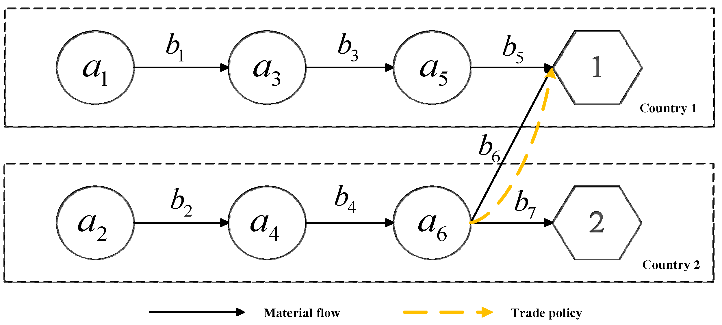
To study the dynamic evolution of inter-chain competition in cross-border supply chains, we consider a scenario in which there are three representative PM chains between two countries of product (country 1 and country 2), as shown in Figure 1. Among these three PM chains, two represent nonmultinational PM chains within each country, and one represents a multinational supply chain symbolizing the trade relationship between the two countries. Without a loss of generality, these three supply chains succinctly describe the interactive relationships among cross-border supply chains.
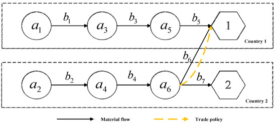
Figure 1.
Cross-border supply chain of countries 1 and 2 for product .
The three-tier PM chain is shown in Figure 1, where , , and are the suppliers of raw materials, upstream manufacturers, and downstream manufacturers, respectively; , , and denote the links where the flow of material occurs; and 1 denotes that the target market of the PM chain is country 1.
Let represent the set of all PM chains as shown in Figure 1, where and . Let represent the cross-border supply chain as a whole, where , , and denote the set of all firms (circles), all links (black arrow lines), and all consumer markets (hexagons), respectively. Thus, , , and .
We can conclude that every PM chain is directed toward a certain market, and the product cannot be completed if any firm or link is removed from the PM chain. Thus, the consideration of one PM chain as a decision-making unit in a supply chain game is reasonable.
To increase the number of local jobs and to support local industries, countries usually implement trade policies related to imported and exported products. Therefore, subsidies and tariffs are imposed on the cross-border links, which are represented as yellow, dashed lines in Figure 1. is a cross-border PM chain, where is a cross-border link.
Each firm faces production costs. At the same time, transaction costs occur at the links with positive material flow, including distribution and transportation costs [4]. In addition to transaction costs, trade costs occur at the cross-border links, which include subsidies and tariff costs.
2.2. Model Formulation
The main symbols used in the establishment of the discrete dynamical model for cross-border supply chains are provided in Table 1.

Table 1.
Key notations.
In a cross-border supply chain, if two PM chains are oriented toward the same market or contain the same firms, they will directly compete in that market or share the resources offered by those firms. That is, there exists a competitive relationship between two PM chains when . Taking Figure 1 as an example, we can see , which indicates that PM chains and compete directly in country 1, and there is a direct competitive relationship between PM Chains and . However, , which indicates that there is no direct competition between PM chains and .
Thus, the inter-chain relationships in Figure 1 result in direct competition among the three PM chains. The competitive relationships among the three players are depicted in Figure 2, where a PM chain represents a game player.
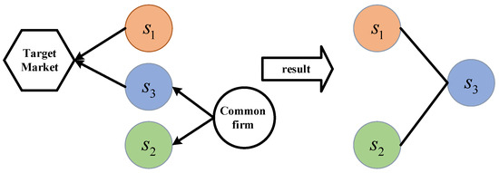
Figure 2.
The competitive relationship between the cross-border supply chains.
Three PM chains compete in a Nash–Cournot pattern to meet the consumer demand in the market. They produce product , and their strategy set involves selecting the optimal output level, with decisions occurring within a discrete period of time . Let denote the set of output quantities for , where . We assume that is sold at the market-clearing price. Then, the market’s demand equals the output quantity of by PM chains oriented to the market. When the output quantity of is , the total output quantity of the final product delivered to market is , where represents the set of all PM chains oriented to market . Thus, in Figure 1, the demand of the market 1 (i.e., country 1) is and that of market 2 (country 2) is .
We assume that the sensitivity of the price to demand equals 1. The inverse demand functions for the three PM chains are defined as follows:
where is interpreted as the maximum price of the final products P*, for market j; represents the substitutability of the final products produced by two countries.
In the supply chain for product , firm is responsible for providing the corresponding intermediate material. Let represent the quantity of intermediate material provided by firm for 1 unit of final product . For example, a screw producer, firm , participates in a PM chain for an automobile tire. Four screws are needed in one tire (), and firm is required to deliver screws for the PM chain when the output quantity of the tire is . Thus, the output quantity of each firm () in PM chain can be represented as .
Here, is a binary variable. If the firm participates in PM chain , then , otherwise .
Firm may participate in various PM chains. Thus, the total output quantity of firm equals the sum of its own output quantities for all PM chains in which it participates.
In a complex supply chain system, a firm’s increase in output quantity per unit tends to result in a nonlinear increase in production costs. In addition, there may be diseconomies of scale phenomena that occur when the scale of each firm expands to a certain extent. Thus, it is appropriate to adopt the quadratic cost function as the production cost function [34]. We can determine the production cost function of firm in the PM chain using the following:
where represents the marginal cost of production of firm .
The output quantity of the front-end firm of link determines the material flow of the link. However, the output quantity of firm is in turn determined by the output quantity of the PM chain to which the firm belongs. Therefore, the material flow of each link can be determined by tracing back the output quantity of . For example, the output quantity of for PM chain , which is , determines the output of firm as and the output of firm as . Then, the front-end firm for link determines the material flow for link as ; the front-end firm determines the material flow for link as . To ascertain the relationships between firms and links, we use the binary variable to indicate that firm is the front-end firm of link and to indicate that firm is not the front-end firm of link . Then, the material flow of link in PM chain , , can be expressed as follows:
The total material flow of each link () may be diverted and distributed to multiple end markets of downstream manufacturers. Therefore, the overall flow of material at each link () can be denoted as follows:
Transaction costs occur at the links with a positive material flow. There may be diseconomies of scale when the transaction scale expands to a certain extent. Therefore, the transaction cost function of link can be assumed to be quadratic in form.
Here, is the marginal transaction cost for link .
Under the subsidy regime, we assume that country 2 imposes a direct subsidy, , on the final product exported to country 1. For instance, in Beijing, China, there is a program to encourage the export of electromechanical products and enhance the international competitiveness of related enterprises. It involves the provision of uncompensated financial assistance, not exceeding RMB 500,000, for the export of electromechanical products. Similarly, the European Union’s agricultural subsidy policy directly subsidizes agricultural exports within the EU region [35]. Under the tariff regime, a unit tariff of occurs on the final product imported from country 2. For the cross-border links, we assume that the tariff cost is proportional to the material flow of the links [4]. Thus, the trade cost on link can be assumed as follows:
where is a binary variable indicating whether a trade policy impacts the link. If yes, ; otherwise, .
On the basis of the above analysis, the total cost of link can be described as follows:
The total cost of PM chain can be defined as follows:
where is the set of all firms that participate in PM chain , and is the set of all links participating in PM chain .
According to (12), the total cost of the three PM chains (, , and ) can be given, respectively, as follows:
Accordingly, the profits of the three PM chains (, , and ) can be given as follows:
where
In the Cournot model, each PM chain is aware of the output level of the other PM chains. When making output decisions, they can observe the total output of the market, as well as the output of other supply chains. This allows each PM chain to make optimal production decisions based on complete information. However, in a real-world market, the game among PM chains is ongoing. Therefore, decision-making by PM chains is a long-term repetitive dynamic process characterized not only by adaptability but also by long-term memory. We assume that all firms are bounded rational. That is, if the estimated marginal profit is negative (positive) in period T, the supply chain firm will reduce (increase) its output quantity in period T + 1. Such adjustments will be reflected in the output of final product in the PM chain . Therefore, all PM chains in Figure 1 are bounded rational. Let represent the output adjustment speed of PM chain . Then, the output adjustment process for PM chain can be expressed as follows:
where denotes the marginal profit function of the PM chain in period T.
By substituting Equation (20) into Equation (19), the discrete dynamical model for the inter-chain output game of the studied supply chain can be obtained as follows:
where
3. Dynamical Analysis for the Model
In the discrete dynamical model (21), by setting , we can obtain the eight equilibrium solutions:
where
, , and are boundary equilibrium points and non-negative; when , is a boundary equilibrium point and non-negative; when , is a boundary equilibrium point and non-negative; when and , is a boundary equilibrium point and non-negative; when and , is an interior equilibrium point and non-negative.
The Jacobian matrix of the complex dynamical model (21) is as follows:
where .
By analyzing the characteristic roots of the Jacobian matrix (22), the stability of the system can be judged. When the absolute values of all characteristic roots are strictly less than 1, the equilibrium point tends to be stable, and the equilibrium point is the Nash equilibrium point of the discrete dynamical model (21) [7].
To discuss the stable region of the discrete dynamical model (21), we substitute the Nash equilibrium points into the Jacobian matrix (22). The characteristic polynomial is obtained as follows:
The discrete dynamical model (21) is also a three-dimensional discrete dynamical system. According to the Jury’s criterion [36], the discrete dynamical system (21) will stabilize asymptotically if the following conditions are satisfied.
4. Numerical Simulations
We assume that in terms of production costs, the marginal production cost in the importing country (country 1) is higher than that in the exporting country (country 2). In terms of transaction costs, the marginal transaction cost of the cross-border links is higher than that of domestic links. For the purpose of comparative analysis, we examine an initial case in which country 1 does not impose tariffs on product imported from country 2. On the basis of these considerations and with reference to Zhang et al. [32] and Feng et al. [4], the following simulation parameters are assumed:
We assume that the suppliers of raw material and the upstream manufacturers require 2 units of materials to produce 1 unit of final product , as shown in Table 2. If a firm participates in chain , a value is provided; otherwise, nonparticipation is represented by “-”.
Table 2.
List of materials required by each firm.
The equilibrium solutions of the complex dynamical system (21) are , , , , , , , and .
By substituting the above solution into the Jacobian matrix (22), we can observe that only the characteristic roots of are less than 1. Therefore, is the unique Nash equilibrium point of the complex dynamical system (21).
The Jacobian matrix at point is given by the following:
The characteristic polynomial can be calculated as Equation (23). Where
According to the Jury criterion (24), the stable region of is shown in Figure 3.
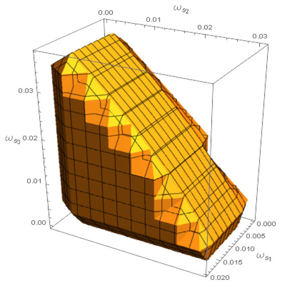
Figure 3.
The system’s stable region of output adjustment speeds , , and .
No matter the initial output level of the PM chain, when the values of the output adjustment speed are within the yellow region shown in Figure 3, the output level will eventually stabilize at . If not, complex behaviors like bifurcation and chaos will occur.
4.1. Bifurcation and Chaos Simulations
4.1.1. The Influence of Output Adjustment on the System
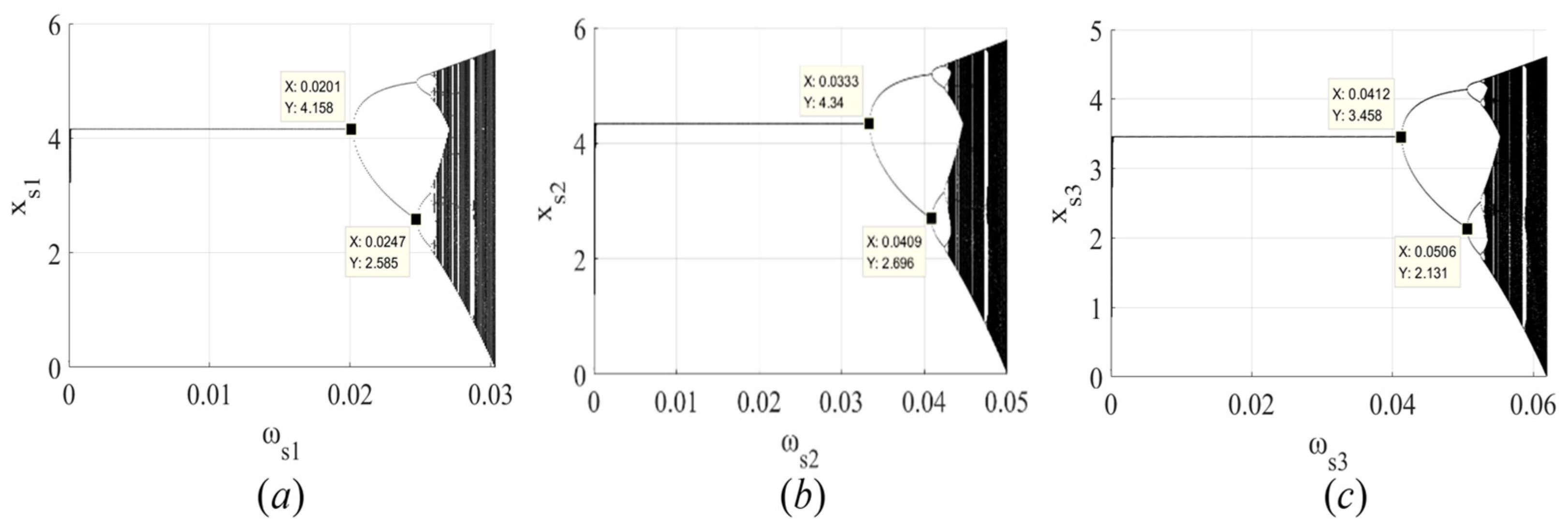
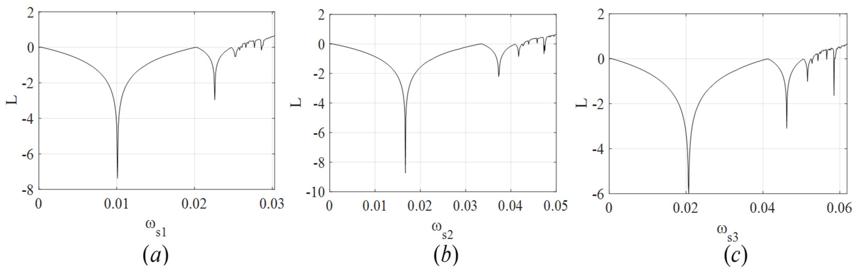
To obtain the bifurcation diagrams of the output decisions of PM chain with respect to its own adjustment speed , we fix the output adjustment speed of the other PM chains at . The results are shown in Figure 4. Additionally, we calculate the maximum Lyapunov exponent, which is an indicator of the system’s stability, and plot its variation in Figure 5.
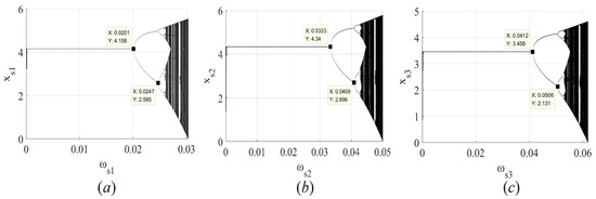
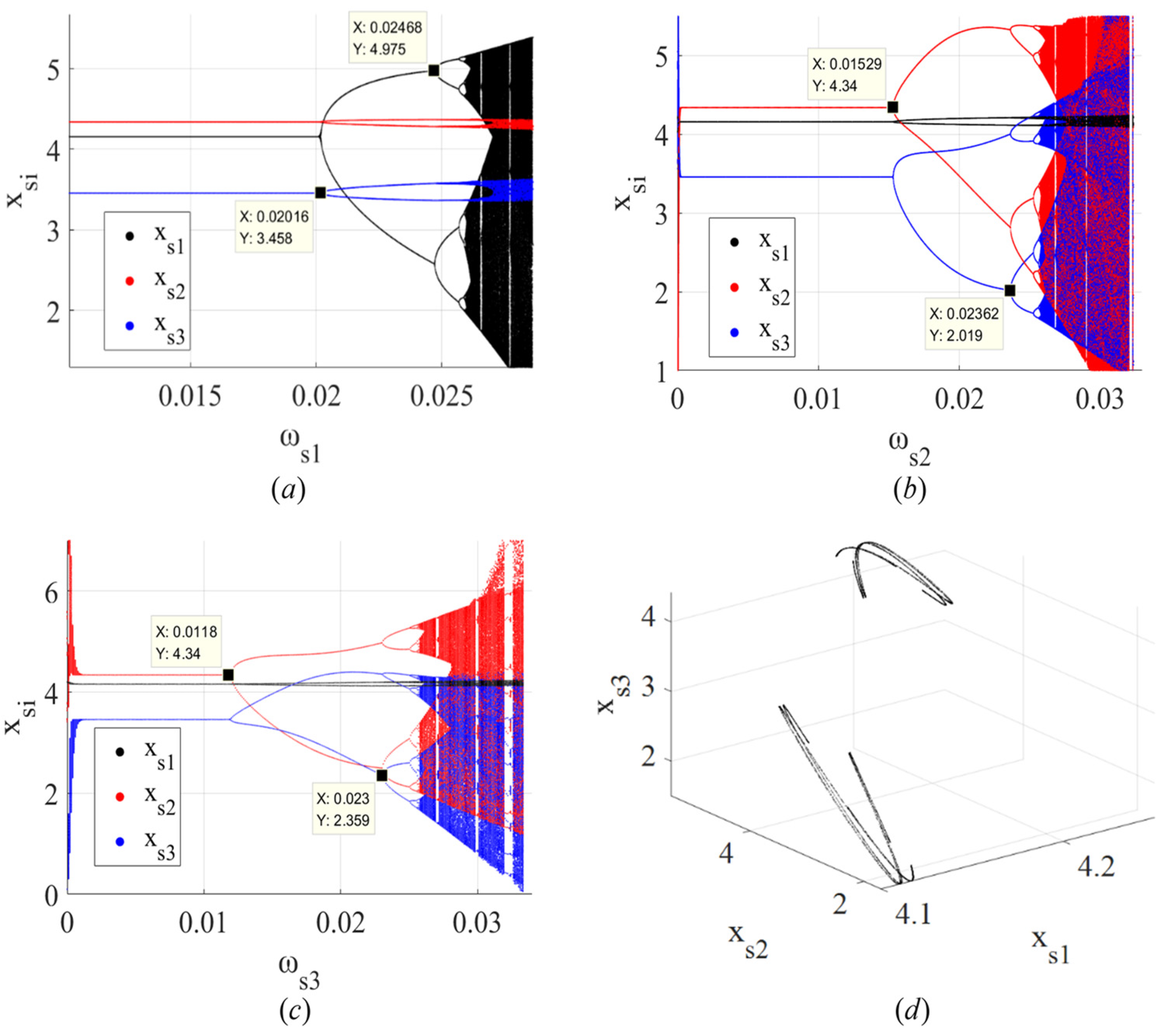
Figure 4.
(a) Bifurcation diagram of the output of with respect to ; (b) bifurcation diagram of the output of with respect to ; (c) bifurcation diagram of the output of with respect to .
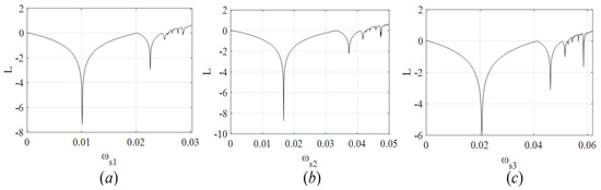
Figure 5.
(a) Maximum Lyapunov exponent of the output of with respect to ; (b) maximum Lyapunov exponent of the output of with respect to ; (c) maximum Lyapunov exponent of the output of with respect to .
In Figure 4a and Figure 5a, when (i.e., the Lyapunov exponent is negative), the output level of the PM chain is stable; when (i.e., the Lyapunov exponent is zero), the output level of occurs at the bifurcation; when and (i.e., the Lyapunov exponent is zero), the output level of occurs at the bifurcation again. Therefore, is the two-periodic orbit, and is the four-periodic orbit. In addition, when (i.e., the Lyapunov exponent is positive), there is an emergence of the chaotic state of the output of . Similar phenomena can also be observed in Figure 4b,c and Figure 5b,c.
Therefore, as the output adjustment of each PM chain is continuously increasing, the output levels of the three PM chains show stability, period-doubling bifurcations, and eventually reach a chaotic state.
To explore the influence of output adjustments on the system (21), we fix and , and the bifurcation diagram of the system is shown in Figure 6a. The bifurcation diagrams created by fixing other parameter combinations are shown in Figure 6b–d and show the chaotic attractor of the system.
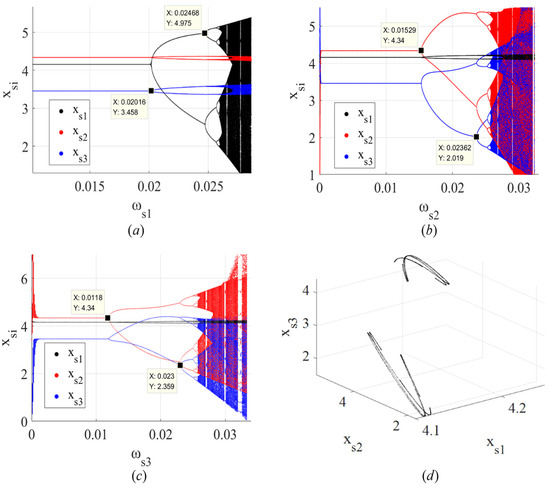
Figure 6.
(a) Bifurcation diagram of the outputs of , , and with respect to when and ; (b) bifurcation diagram of the outputs of , , and with respect to when and ; (c) bifurcation diagram of the outputs of , , and with respect to when and ; (d) chaotic attractor of the system at , , and .
Figure 6a shows that when , the system is in a stable state. When , bifurcation occurs in the system for the first time and enters a two-period orbit. When further increases to , bifurcation occurs in the system a second time and enters a four-period orbit. Similarly, when , bifurcation in the system occurs for the third time. As continues to increase, the system eventually enters a chaotic state.
Figure 6b and Figure 6c show that as and increase, the system reaches a stable state and a period-doubling bifurcation and chaotic state, respectively, similar to Figure 6a.
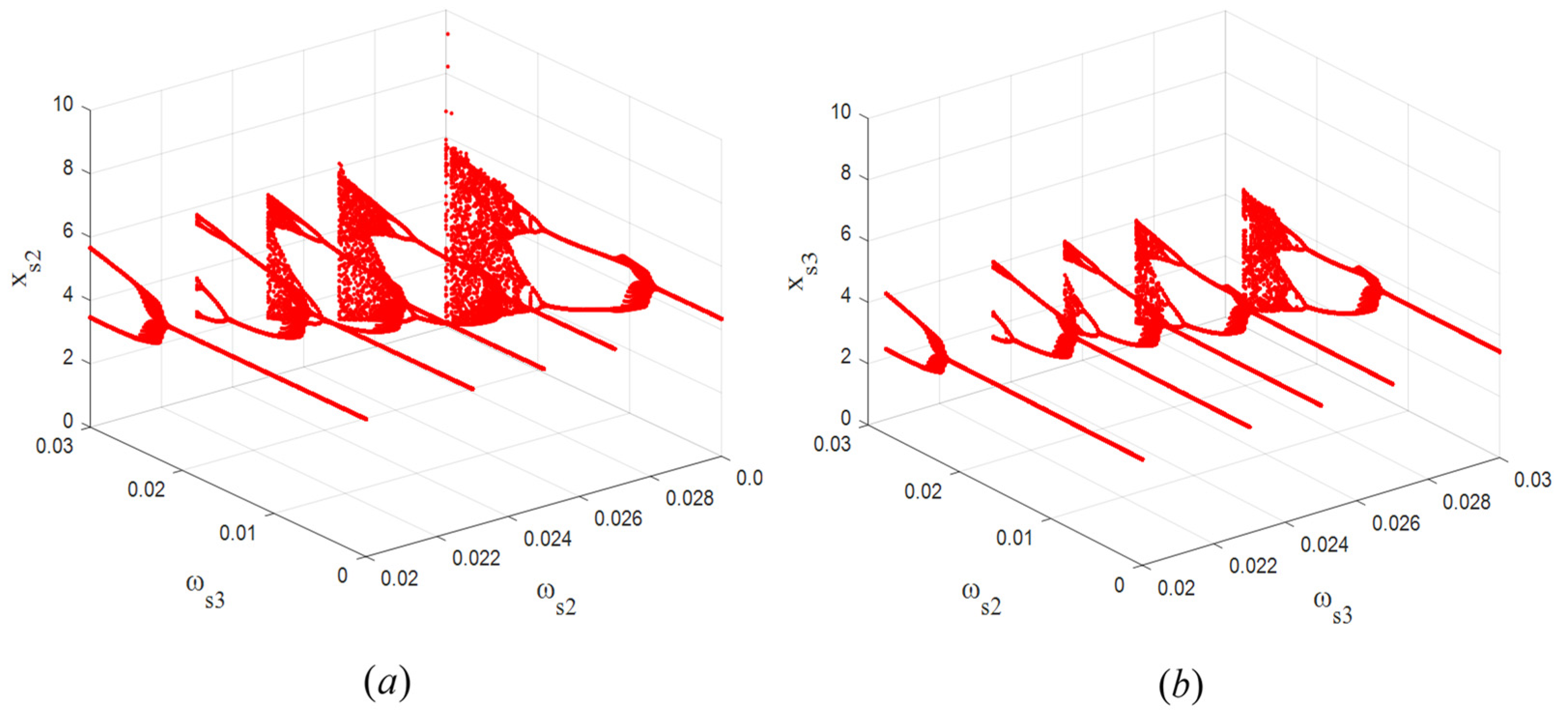
Figure 7 shows the bifurcation and chaos phenomena in three-dimensional space with respect to and . With the increase in the output adjustment speed of , the stable range of will decrease, and will enter a chaotic state. Similarly, an increase in will reduce the stable range of and cause the output level of to eventually enter a state of bifurcation or even chaos.
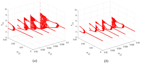
Figure 7.
(a) Three-dimensional bifurcation diagram of the output of with respect to and ; (b) three-dimensional bifurcation diagram of the output of with respect to and .
We can conclude that the system (21) will lose stability as the output adjustment speed increases. When the adjustment speed of any PM chains in the studied supply chain surpasses a specific threshold, the system will eventually enter a chaotic state. This phenomenon leads to fluctuations not only in the output of one PM chain but also in the output of the entire system. This causes further fluctuations in the market. Therefore, in order to avoid market fluctuations as much as possible, it is crucial that each PM chain makes an effort to control the adjustment speed of the output.
4.1.2. Influence of Output Adjustment on the System
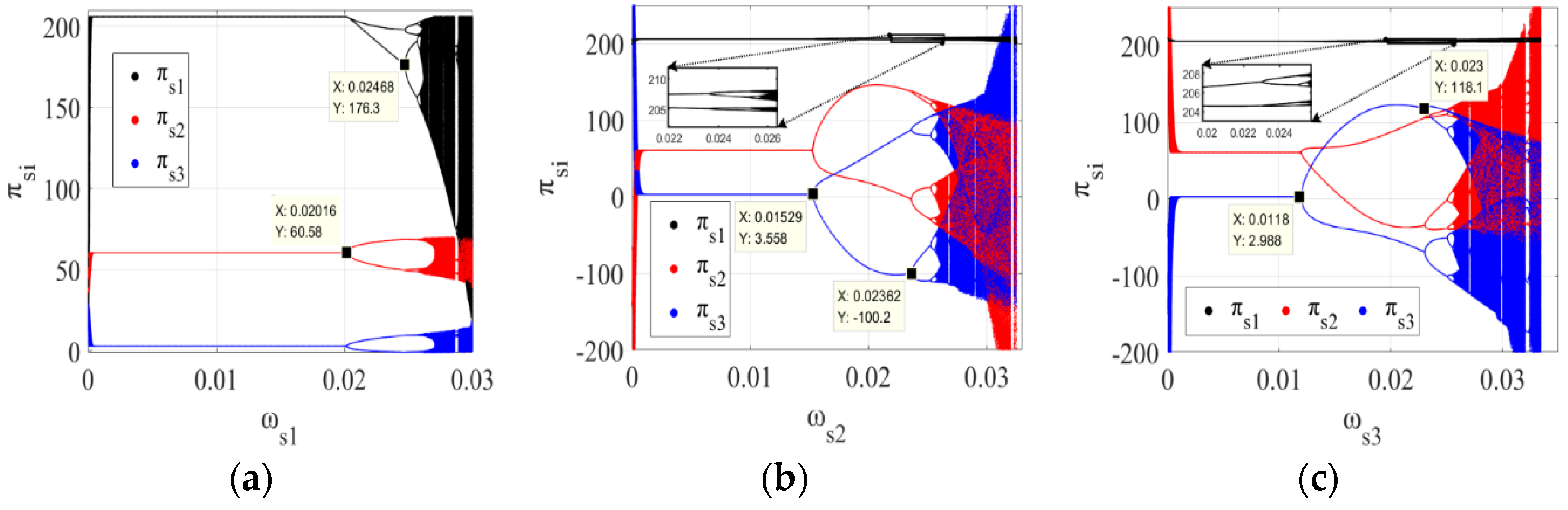
When the adjustment speed of the output surpasses a specific threshold, the output level of the system (21) will enter a chaotic state, which also affects the profits of each PM chain. Thus, to explore the influence of the output adjustment on the system’s profits, we fixed the same parameters as in Figure 6a, Figure 6b, and Figure 6c, and the results are shown in Figure 8a, Figure 8b, and Figure 8c, respectively. The intervals of the stable, period-doubling bifurcation, and chaotic states shown in Figure 8 are consistent with Figure 6.

Figure 8.
(a) Bifurcation diagram of the profits of , , and with respect to when and ; (b) bifurcation diagram of the profits of , , and with respect to when and ; (c) bifurcation diagram of the profits of , , and with respect to when and .
Figure 8 shows that the system’s profits change from a stable to period-doubling bifurcation state and eventually enter a chaotic state as the adjustment speeds of , , and increase, respectively. The long-term development of the three PM chains will be severely hampered by the fluctuation in profits. Furthermore, the profits of PM chain , as shown in Figure 8a, fall after entering a period-doubling bifurcation state, which suggests that an excessive output adjustment speed not only destabilizes but also decreases the profits of PM chain . To protect the profits of the entire system, each PM chain firm should make suitable adjustments to the speed of output.
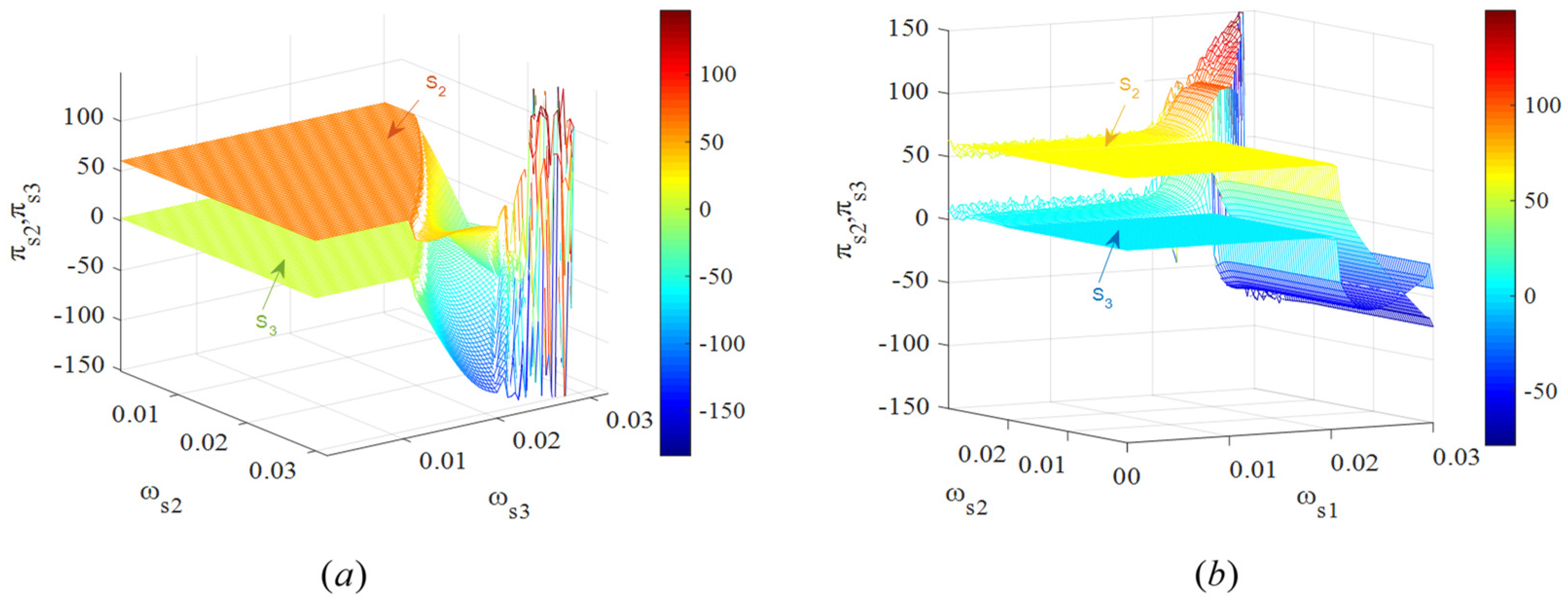
Figure 9 shows the three-dimensional profits diagrams of and with respect to , and , . In Figure 9a, when is small, the increase in does not destabilize the profits of and . However, when is large, the increase in will cause the profits of both and to decline and eventually enter a chaotic state. This shows that for an exporting country, when the output adjustment speed of export products is too high, the profits of the supply chain in the exporting country will decline. This is unfavorable for exporting countries, so they should opt for a smaller adjustment speed for the quantity of exports. In Figure 9b, when the value of is relatively small, the increase in results in an overall rise in the profits of and . However, when is large, the increase in will cause the profits of both and to decline. By comprehensively analyzing Figure 9a,b, we can conclude that, whether making decisions on the export quantity or the level of domestic output, the exporting country should adopt a relatively smaller output adjustment speed.
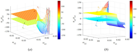
Figure 9.
(a) Profits of and with respect to and when ; (b) profits of and with respect to and when .
4.1.3. Influence of Tariffs on the System
The analysis above was based on the assumption that country 1 does not impose tariffs on country 2. To investigate the influence of tariffs on system dynamics, we conducted simulations with different tariff levels, which are represented by the parameter . The results are presented in Figure 10a,b.
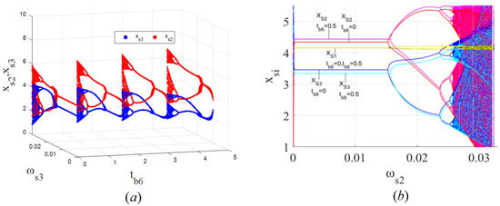
Figure 10.
(a) Three-dimensional bifurcation diagram of the outputs of and with respect to and when and ; (b) bifurcation diagram of the outputs of the system with respect to and when and .
Figure 10a shows a three-dimensional bifurcation diagram of and with respect to and . When the unit tariff cost increases, the equilibrium of the output level of PM chain declines, and the stable ranges of and are reduced. It is more challenging for products to enter overseas markets, and the supply chain of imported goods is more unstable, when higher tariffs are imposed on the products.
Figure 10b shows that when the adjustment speed rises, changes in the unit tariff cost have no effect on the dynamic evolution of the PM chain , but they influence and . As the unit tariff cost increases from 0 to 0.5, the equilibrium output level of PM chain increases, while that of the PM chain declines. Additionally, as the unit tariff cost rises, there is an expansion in the stable range of PM chains and . This indicates that for the tariff-imposing country (country 1), although the increase in tariffs can protect domestic producers, it can also lead to the expansion of the stable range of the PM chain in the product-exporting country (country 2). Thus, when the output adjustment speed surpasses a specific threshold, the PM chains of country 2 enter a bifurcation state or even a chaotic state, whereas the PM chains of country 1 exhibit sustained stability. This is unfavorable for the tariff-imposing country (country 1). Moreover, the likelihood of such an adverse situation increases as tariffs increase. To prevent fluctuations in its own market, the tariff-imposing country should impose appropriate tariffs.
4.1.4. Influence of Initial Values on the System
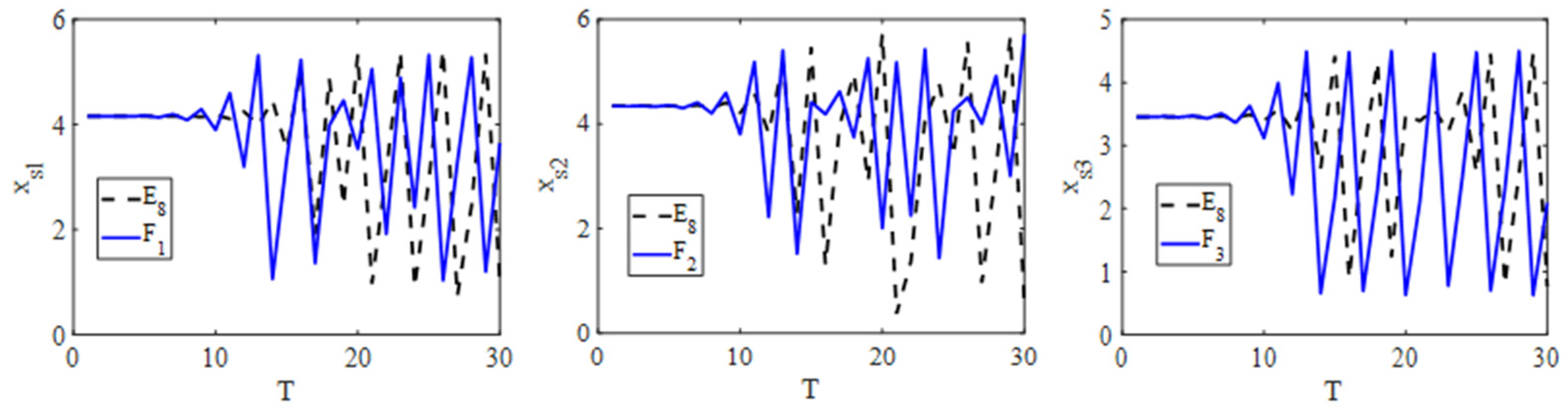
In Figure 3, we can see that when the adjustment speeds of , , and are , , and , respectively, the system is in a chaotic state. This means that at these adjustment speeds, the output level of each PM chain will fluctuate unpredictably over time. To explore the influence of the initial values on the chaotic state of the system, we made slight adjustments to the equilibrium output level of the three PM chains denoted as , , and , and plotted a time series graph, as shown in Figure 11.

Figure 11.
Time series graph of the output levels of , , and under different initial values.
Figure 11 shows that during the early stages of the system’s evolution, the output levels based on equilibrium point , as the initial value, exhibited relatively stable changes over time. However, when , , and were used as initial values, the trajectory of the output levels showed significant fluctuations. As the system continuously evolves, the trajectories of the output levels based on equilibrium point , as the initial value, differ significantly from the trajectories based on , , and as initial values. Overall, we can conclude that the chaotic state of the system (21) is sensitive to initial values, and even slight differences in the initial conditions can lead to substantial variations in the evolution of the system (21).
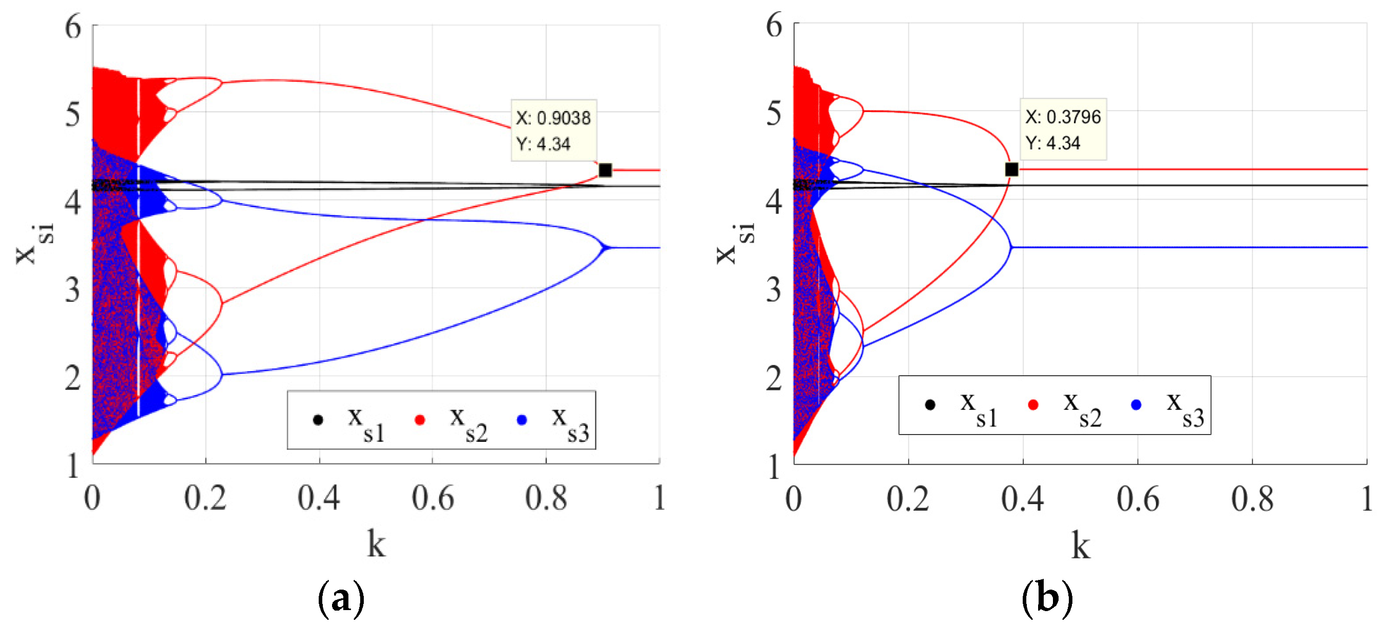
4.2. Chaos Control
On the basis of the above analysis, we can conclude that chaos will cause damage to the system, which causes profits to fall and fluctuate irregularly. We applied the delayed feedback control method to control the system’s chaotic behavior [37]. In our study, a PM chain is a game player, and the firms in it all make efforts to achieve an output of for the final product. Therefore, firms in the PM chain have the same output adjustment speed and control factor for delayed feedback decision-making. When the time delay of PM chain is chosen as 1, the control system can be described as follows:
where , is a controlling factor.
When the time delay of PM chains , , and are all chosen as 1, the control system can be represented as follows:
where , .
Figure 12 shows that the system’s chaotic state stabilized with an increase in , which indicates that the method of delayed feedback control is effective for controlling chaos in the system (21). This further indicates that a PM chain firm should adjust its output level by considering not only the last period’s profits as a benchmark but also the profits of further previous periods as a reference to improve the stability when making decisions. Comparing Figure 12a and Figure 12b, we also notice that the transition from a chaotic state to stable state in Figure 12b occurred faster than Figure 12a, which indicates that each PM chain firm in the system should adopt the delayed feedback control method to adjust its level of output.

Figure 12.
(a) Effect of control factor on the output with a delayed feedback control of ; (b) effect of control factor on the output with delayed feedback controls of , , and .
5. Conclusions
We established a discrete dynamical model for an output game from the perspective of inter-chain competition and obtained the Nash equilibrium point and its stable region. From the numerical simulations, bifurcation diagrams, maximum Lyapunov exponents, and time series graphs are presented to illustrate the complex dynamic behaviors of the dynamical model.
Our research showed that the output adjustment speed has a significant impact on the stability of the whole supply chain system. It can magnify fluctuations in the level of output in a supply chain system and can eventually lead to a chaotic state when the output adjustment speed surpasses a specific threshold. Supply chain firms need to pay attention to whether the output adjustment speed is excessive, as this will not only cause instability in the supply chain in which it participates but also reduce the profits of the supply chain in which it participates. To protect their own profits, each supply chain firm should adjust its output level to a lower speed. The increase in tariffs will expand the stable range of the PM chain in the product-exporting country. Therefore, to prevent fluctuations in its own market, governments of tariff-imposing countries should impose appropriate tariffs. Additionally, the chaotic behavior of the system is sensitive to the initial level of output. Each PM chain should evaluate the potential impacts of different initial output values carefully. When the market is in a chaotic state, applying the method of delayed feedback control would have an effect on the system stability. To maintain system stability and prevent profit loss, it is particularly important for each PM chain firm to adjust its output level by considering not only the profits of the last period but also the profits of further previous periods as references. Government organizations should also actively introduce relevant policies to regulate the phenomena of chaos.
To better explore the nature of solutions of inter-chain competition and the complexity of dynamic evolution, our study selectively focused on three representative supply chains within a global supply chain network. Therefore, there are some limitations of this study, and a great deal of work is yet to be completed. More complex scenarios, such as the export of raw materials or intermediate products, as well as special cases like tariff exemptions between countries with technological disparities, were not considered in our model. Interestingly, if a company engages in the export of raw materials or intermediate materials, a new PM chain would be added to the game system based on our model. Subsequently, this new PM chain must be incorporated into the nonlinear dynamical system model, leading to an increase in model’s dimensionality and analytical complexity. Thus, enriching our model is an interesting subject for future study.
Author Contributions
Conceptualization, F.-J.X. and L.-Y.W.; methodology, L.-Y.W. and S.-Y.W.; software, L.-Y.W. and S.-Y.W.; validation, F.-J.X. and L.-Y.W.; formal analysis, L.-Y.W.; investigation, L.-Y.W. and Y.-F.L.; resources, Y.-F.L.; writing—original draft preparation, F.-J.X. and L.-Y.W.; writing—review and editing, F.-J.X., L.-Y.W. and S.-Y.W.; visualization, L.-Y.W.; supervision, F.-J.X. and S.-Y.W.; project administration, F.-J.X.; funding acquisition, Y.-F.L. and S.-Y.W. All authors have read and agreed to the published version of the manuscript.
Funding
This research was funded by the National Social Science Fund of China (grant no. 18XGL001), the Natural Science Basic Research Plan in Shaanxi Province of China (grant no. 2023-JC-QN-0261), and the Shaanxi Provincial Education Department (23JK0675).
Data Availability Statement
Data are contained within the article.
Acknowledgments
The authors are grateful to the editors and anonymous reviewers for providing valuable comments.
Conflicts of Interest
The authors have no conflicts of interest related to the publication of this paper.
References
- Kang, K.; Zhao, Y.; Zhang, J.; Qiang, C. Evolutionary game theoretic analysis on low-carbon strategy for supply chain enterprises. J. Clean. Prod. 2019, 230, 981–994. [Google Scholar] [CrossRef]
- Korpeoglu, C.G.; Körpeoğlu, E.; Cho, S.H. Supply chain competition: A market game approach. Manag. Sci. 2020, 66, 5648–5664. [Google Scholar] [CrossRef]
- Yuan, X.; Bi, G.; Fei, Y.; Liu, L. Supply chain with random yield and financing. Omega 2021, 102, 102334. [Google Scholar] [CrossRef]
- Feng, P.; Zhou, X.; Zhang, D.; Chen, Z.; Wang, S. The impact of trade policy on global supply chain network equilibrium: A new perspective of product-market chain competition. Omega 2022, 109, 102612. [Google Scholar] [CrossRef]
- Li, Y.; Chen, B.; Chen, G.; Wu, X. The global oil supply chain: The essential role of non-oil product as revealed by a comparison between physical and virtual oil trade patterns. Resour. Conserv. Recycl. 2021, 175, 105836. [Google Scholar] [CrossRef]
- Ivanov, D.; Dolgui, A. Viability of intertwined supply networks: Extending the supply chain resilience angles towards survivability. A position paper motivated by COVID-19 outbreak. Int. J. Prod. Res. 2020, 58, 2904–2915. [Google Scholar] [CrossRef]
- Lou, W.; Ma, J. Complexity of sales effort and carbon emission reduction effort in a two-parallel household appliance supply chain model. Appl. Math. Model. 2018, 64, 398–425. [Google Scholar] [CrossRef]
- Ma, J.; Wang, Z. Optimal pricing and complex analysis for low-carbon apparel supply chains. Appl. Math. Model. 2022, 111, 610–629. [Google Scholar] [CrossRef]
- Giri, B.C.; Bardhan, S.; Maiti, T. Coordinating a three-layer supply chain with uncertain demand and random yield. Int. J. Prod. Res. 2016, 54, 2499–2518. [Google Scholar] [CrossRef]
- Giri, B.C.; Bardhan, S. Sub-supply chain coordination in a three-layer chain under demand uncertainty and random yield in production. Int. J. Prod. Econ. 2017, 191, 66–73. [Google Scholar] [CrossRef]
- Zhang, S.; Dan, B.; Zhou, M. After-sale service deployment and information sharing in a supply chain under demand uncertainty. Eur. J. Oper. Res. 2019, 279, 351–363. [Google Scholar] [CrossRef]
- Nouira, I.; Hammami, R.; Arias, A.F.; Gondran, N.; Frein, Y. Olive oil supply chain design with organic and conventional market segments and consumers’ preference to local products. Int. J. Prod. Econ. 2022, 247, 108456. [Google Scholar] [CrossRef]
- Hu, B.; Feng, Y. Optimization and coordination of supply chain with revenue sharing contracts and service requirement under supply and demand uncertainty. Int. J. Prod. Econ. 2017, 183, 185–193. [Google Scholar] [CrossRef]
- Kerkkamp, R.B.O.; van den Heuvel, W.; Wagelmans, A.P.M. Two-echelon supply chain coordination under information asymmetry with multiple types. Omega 2018, 76, 137–159. [Google Scholar] [CrossRef]
- Raza, S.A. Supply chain coordination under a revenue-sharing contract with corporate social responsibility and partial demand information. Int. J. Prod. Econ. 2018, 205, 1–14. [Google Scholar] [CrossRef]
- Ranjan, A.; Jha, J.K. Pricing and coordination strategies of a dual-channel supply chain considering green quality and sales effort. J. Clean. Prod. 2019, 218, 409–424. [Google Scholar] [CrossRef]
- Wang, L.; Song, H.; Wang, Y. Pricing and service decisions of complementary products in a dual-channel supply chain. Comput. Ind. Eng. 2017, 105, 223–233. [Google Scholar] [CrossRef]
- Asl-Najafi, J.; Yaghoubi, S.; Zand, F. Dual-channel supply chain coordination considering targeted capacity allocation under uncertainty. Math. Comput. Simul. 2021, 187, 566–585. [Google Scholar] [CrossRef]
- Li, M.; Mizuno, S. Dynamic pricing and inventory management of a dual-channel supply chain under different power structures. Eur. J. Oper. Res. 2022, 303, 273–285. [Google Scholar] [CrossRef]
- Cai, G.G. Channel selection and coordination in dual-channel supply chains. J. Retail. 2010, 86, 22–36. [Google Scholar] [CrossRef]
- Zhou, Y.; Ye, X. Differential game model of joint emission reduction strategies and contract design in a dual-channel supply chain. J. Clean. Prod. 2018, 190, 592–607. [Google Scholar] [CrossRef]
- Nagurney, A.; Dong, J.; Zhang, D. A supply chain network equilibrium model. Transp. Res. Part E Logist. Transp. Rev. 2002, 38, 281–303. [Google Scholar] [CrossRef]
- Nagurney, A.; Besik, D.; Li, D. Strict quotas or tariffs? Implications for product quality and consumer welfare in differentiated product supply chains. Transp. Res. Part E Logist. Transp. Rev. 2019, 129, 136–161. [Google Scholar] [CrossRef]
- Nagurney, A.; Besik, D.; Dong, J. Tariffs and quotas in world trade: A unified variational inequality framework. Eur. J. Oper. Res. 2019, 275, 347–360. [Google Scholar] [CrossRef]
- Yang, Y.X.; Guang, Q.; Zhang, B.Y.; Meng, L.J.; Yu, Y.N. Closed-loop Supply Chain Network Equilibrium Analysis under Carbon Tax Policies. Chin. J. Manag. Sci. 2022, 30, 185–195. [Google Scholar] [CrossRef]
- Zhou, X.Y.; Cao, W.J.; Fu, H.R.; Feng, P.P.; Chai, J. Cross-national supply chain network equilibrium decision of considering product substitution under stochastic demand. Syst. Eng. –Theory Pract. 2022, 42, 2853–2868. [Google Scholar] [CrossRef]
- Xiao, Y.X.; Zhang, R.Q. Supply chain network equilibrium considering coordination between after-sale service and product quality. Comput. Ind. Eng. 2023, 175, 108848. [Google Scholar] [CrossRef]
- McGuire, T.W.; Staelin, R. An industry equilibrium analysis of downstream vertical integration. Mark. Sci. 1983, 2, 161–191. [Google Scholar] [CrossRef]
- Wang, S.; Hu, Q.; Liu, W. Price and quality-based competition and channel structure with consumer loyalty. Eur. J. Oper. Res. 2017, 262, 563–574. [Google Scholar] [CrossRef]
- Fang, Y.; Shou, B. Managing supply uncertainty under supply chain Cournot competition. Eur. J. Oper. Res. 2015, 243, 156–176. [Google Scholar] [CrossRef]
- Zhao, H.; Chen, J.; Ai, X. Contract strategy in the presence of chain to chain competition. Int. J. Prod. Res. 2022, 60, 1913–1931. [Google Scholar] [CrossRef]
- Zhang, D. A network economic model for supply chain versus supply chain competition. Omega 2006, 34, 283–295. [Google Scholar] [CrossRef]
- Counterpoint Quarterly, Global Smartphone Shipments Market Data (Q3 2021–Q2 2023). Available online: https://www.counterpointresearch.com/global-smartphone-share/ (accessed on 17 August 2023).
- Dubiel-Teleszynski, T. Nonlinear dynamics in a heterogeneous duopoly game with adjusting players and diseconomies of scale. Commun. Nonlinear Sci. Numer. Simul. 2011, 16, 296–308. [Google Scholar] [CrossRef]
- Rude, J. Direct and Indirect Export Subsidies. Chapters 2007. Available online: https://www.elgaronline.com/view/9781843769392.00035.xml (accessed on 28 December 2023).
- Jury, E.I.; Paynter, H.M. Inners and stability of dynamic systems. J. Dyn. Sys. Meas. Control 1975, 97, 208. [Google Scholar] [CrossRef]
- Yassen, M.T.; Agiza, H.N. Analysis of a duopoly game with delayed bounded rationality. Appl. Math. Comput. 2003, 138, 387–402. [Google Scholar] [CrossRef]


Disclaimer/Publisher’s Note: The statements, opinions and data contained in all publications are solely those of the individual author(s) and contributor(s) and not of MDPI and/or the editor(s). MDPI and/or the editor(s) disclaim responsibility for any injury to people or property resulting from any ideas, methods, instructions or products referred to in the content. |
© 2024 by the authors. Licensee MDPI, Basel, Switzerland. This article is an open access article distributed under the terms and conditions of the Creative Commons Attribution (CC BY) license (https://creativecommons.org/licenses/by/4.0/).