Mechanisms of Stock Selection and Its Capital Weighing in the Portfolio Design Based on the MACD-K-Means-Mean-VaR Model

Abstract

When designing a stock portfolio, investors must select stocks with different characteristics and increasing price trends and weigh each capital. Both are fundamental to diversifying loss and profit. Therefore, the mechanisms that accommodate both are needed. Based on this, this research aims to design a stock selection and capital weighing mechanism using the MACD-K-means-Mean-VaR model. The moving average convergence–divergence (MACD) is used to analyze stock buying time, providing trend, momentum, and potential price reversal insights. Then, stocks with increasing price trends are clustered using K-means, a grouping simple pattern data method based on specific characteristics. The best stocks from each cluster are capital weighted using the mean value at risk (mean-VaR), a portfolio optimization model adjusting loss possibility to the investor’s acceptance tolerance. The mechanism is then applied to Indonesia’s 100 stock index data to analyze variable sensitivities and compare it with another model. The application reveals that all variables significantly impact portfolio return mean and VaR, suggesting the need for clustering and analyzing stock price movements in stock portfolio design. This research academically develops a portfolio design mechanism by clustering stocks and analyzing price movement trends. It enables investors to practically diversify and choose stocks with increasing price trends, reducing losses and increasing profit opportunities.

1. Introduction

When selecting stocks in portfolio design, diversification should be carried out to manage investment risk wisely [1]. Stock diversification is a stock selection activity based on classifying different characteristics from different clusters. By selecting stocks in different clusters, the returns from the stocks in the portfolio are not highly correlated. It creates a return balance, where if one stock in the portfolio experiences a decline, the potential loss can be offset by positive performance stock in other clusters. In detail, it not only protects against losses but also increases the potential for stable and sustainable returns [2]. 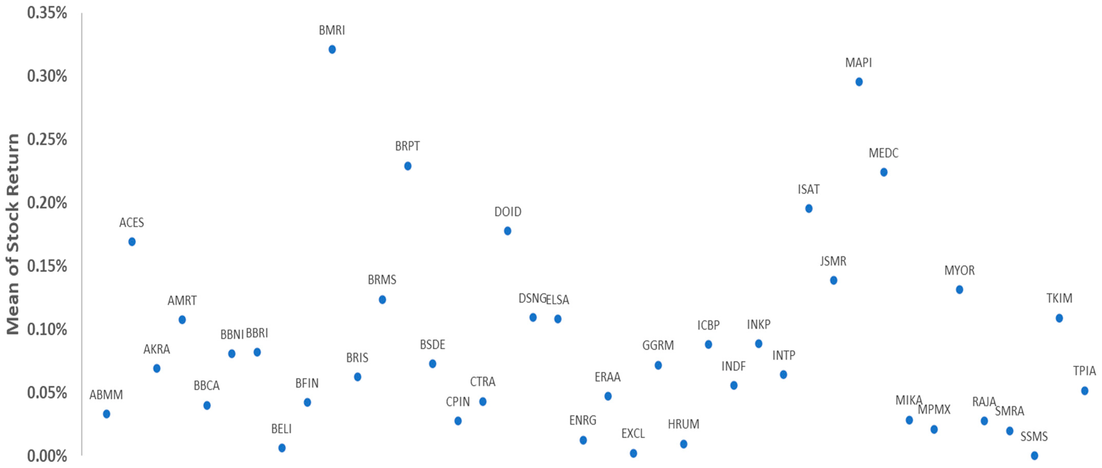Apart from diversification through clustering, analyzing the timing of buying and selling stocks is also important in selecting stocks in portfolio design [3]. The stocks chosen should have buy indications so that the risk of loss can be minimized in the future. Analysis of when to buy and sell stocks can be conducted using daily price data or based on company fundamentals. After the selection of stocks in portfolio design is conducted, the next step is determining the capital weight of each stock within it. Stocks with a large mean of return are not always given a large capital weight, and vice versa. This is because it must be remembered that the mean and variance of returns have in-line properties [4]. Thus, this weighting needs to be conducted carefully. The weighting of stock capital in a portfolio should be carried out based on basic investment objectives, namely maximizing returns and minimizing the risk of loss.

Several studies have discussed the mechanism of stock selection using clusterization. Chen and Huang [5] introduced a clustering-based stock selection mechanism using the K-means algorithm, focusing on attributes such as average return, standard deviation of returns, Treynor index, and turnover rate. Sinha et al. [6] used a genetic algorithm to cluster stocks. Golosnoy and Okhrin [7] developed a mean-variance model involving shrinkage. Ren et al. [8] applied the K-means algorithm to cluster stocks with attribute correlation coefficients. Fleischhacker et al. [9] clustered stock data in the energy sector using the K-means algorithm with the attributes of heat demand, electricity demand, cooling demand, solar PV supply, and solar thermal collector supply. Using the average linkage algorithm and the distinctive features of the correlation coefficient between stock returns, Tola et al. [10] grouped stock data. Musmeci et al. [11] compared the K-medoids, linkage, and directed bubble hierarchical tree approaches using the correlation coefficient attributes of stocks. Hussain et al. [12] proposed two novel methods, namely the Adaptive Neuro-Fuzzy Inference System (ANFIS) and the Induced Ordered Weighted Averaging (IOWA) model, for cluster stocks. Chen et al. [13] and Cheong et al. [14] employed the K-means technique to cluster stock data based on the average return attribute. Khan and Mehlawat [15] employed fuzzy C-means clustering to group stocks into clusters. Then, Sáenz [16] investigated the application of clustering models for stocks to enhance the accuracy of stock price predictions and the performance of trading algorithms.

Meanwhile, several researchers have also analyzed stock price movements. Navarro et al. [17] conducted a price analysis using the moving average convergence–divergence (MACD) approach. Aheer et al. [18] examined price fluctuations using geometric Brownian motion. Subsequently, Sukono et al. [19] analyzed the stock price fluctuations using the ARIMA-GARCH model. Subsequently, Du and Tanaka-Ishii [20] analyzed the movement of stock prices using NEWS-STock space with Event Distribution (NESTED). Chang et al. [21] analyzed price fluctuations using behavioral stock (B-stock). Varga-Haszonits and Kondor [22] examined the price movement, assuming it adheres to the constant conditional correlation GARCH process model provided by Bollerslev. Thuankhonrak et al. [23] conducted a price analysis using the ARIMA and Holt Winter techniques.

Then, in capital weighting, Markowitz [24] introduced the mean-variance capital weighting model in portfolios, which was later transformed into a matrix form for better computing efficiency by Sharpe [25]. This model became the basis for future research, including the capital asset pricing model (CAPM) by Sharpe [26] and the minimax portfolio model by Young [27]. Other researchers have developed models for risk aversion by Björk et al. [28], portfolio mean-variance-skewness by Abdurakhman [29], equilibrium optimizer by Faramarzi et al. [30], multi-objective stochastic linear optimization by Zhou and Li [31], particle swarm optimization by Zhu et al. [32], mean absolute deviation by Kalfin et al. [33] and Ryoo [34], neurodynamic optimization by Wang and Gan [35], behavioral mean-variance and copula behavioral mean-variance by Mba et al. [36], portfolio optimization via deep learning by Du [37], and predictive control models of mean-variance by [38]. Each model has strengths and weaknesses, and their application in various scenarios has led to significant advances in the field. The mean-variance model has been a valuable tool for understanding and optimizing portfolio capital. Ranković [39] introduced a new mean-VaR optimization technique that utilizes a univariate Generalized Autoregressive Conditional Heteroscedasticity (GARCH) volatility model to estimate VaR. Then, Ashrafzadeh [40] presented a hybrid approach that combines a convolutional neural network (CNN) with optimized hyperparameters using particle swarm optimization (PSO) for stock pre-selection. A mean-variance with forecasting (MVF) model is employed for portfolio optimization.

Some gaps from previous research can be used as opportunities for further research. These gaps are considered novel in this research. These gaps are as follows:

(a)

In the clustering aspect, no one has used the K-means method with the mean and value at risk (VaR) attributes of returns from their stocks.

(b)

Regarding capital weighting, no one has used the mean-VaR model involving income tax and transaction cost variables.

(c)

No one has yet combined the MACD method for buying time analysis with the K-means method and the mean-VaR model.

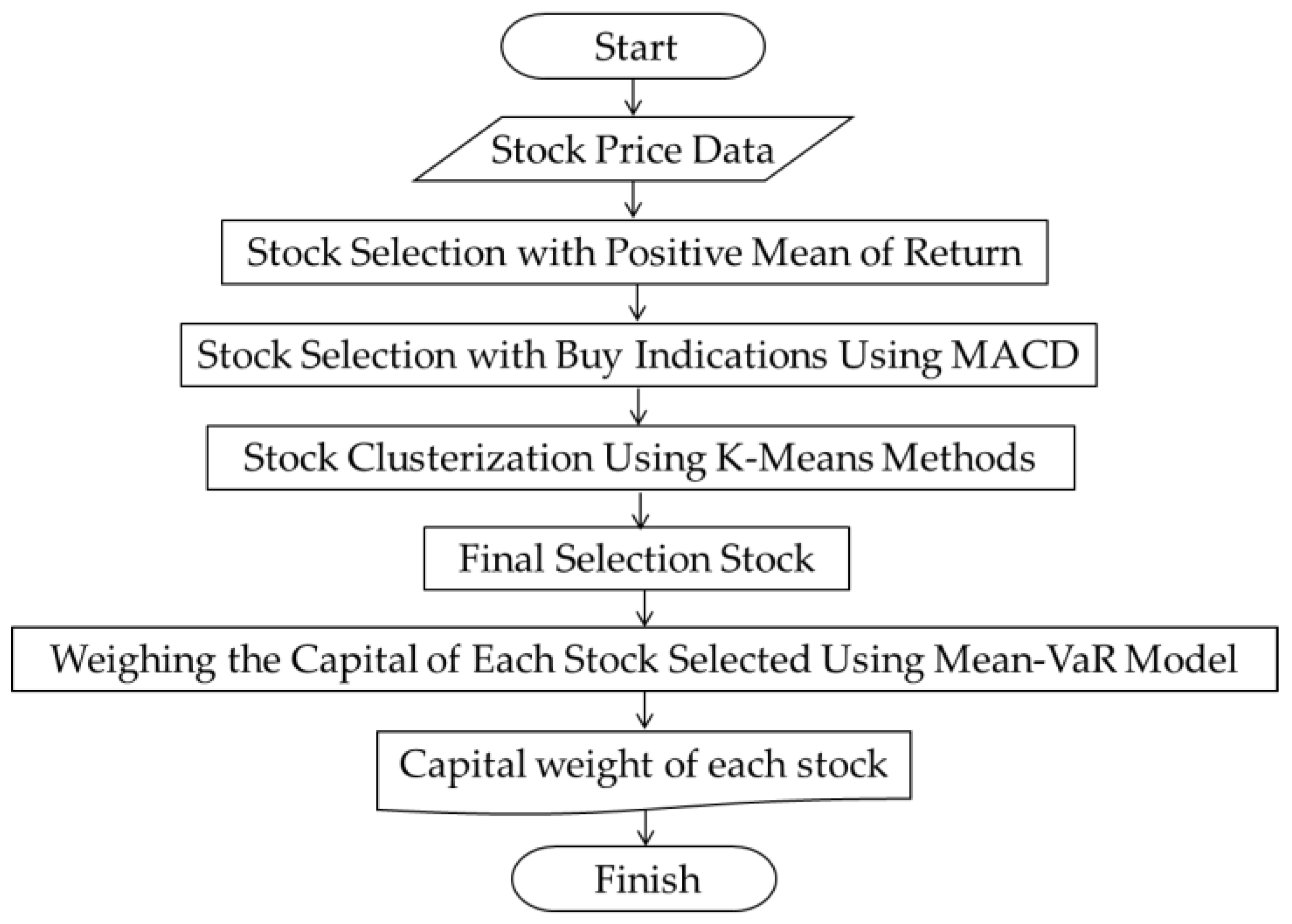
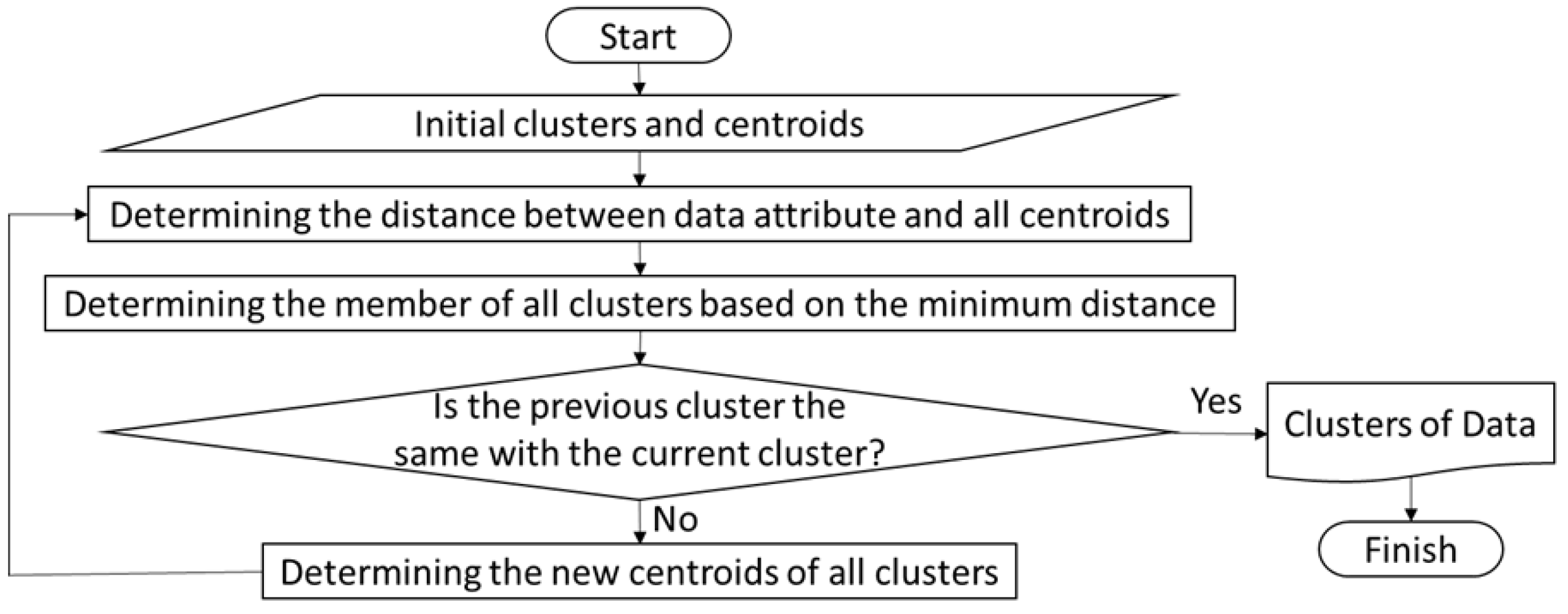
Based on the introduction in this section, this research aims to develop stock selection and capital weighting mechanisms in designing stock portfolios based on clustering and analysis of stock buying times. Clustering was carried out using the K-means method. This method was chosen because of its fast iteration speed, timely efficiency, and simple ability to provide a clear and well-defined cluster solution to help investors understand the relationship patterns between stocks in a portfolio [41]. Then, the time to buy stocks is analyzed using the moving average convergence–divergence (MACD) indication. 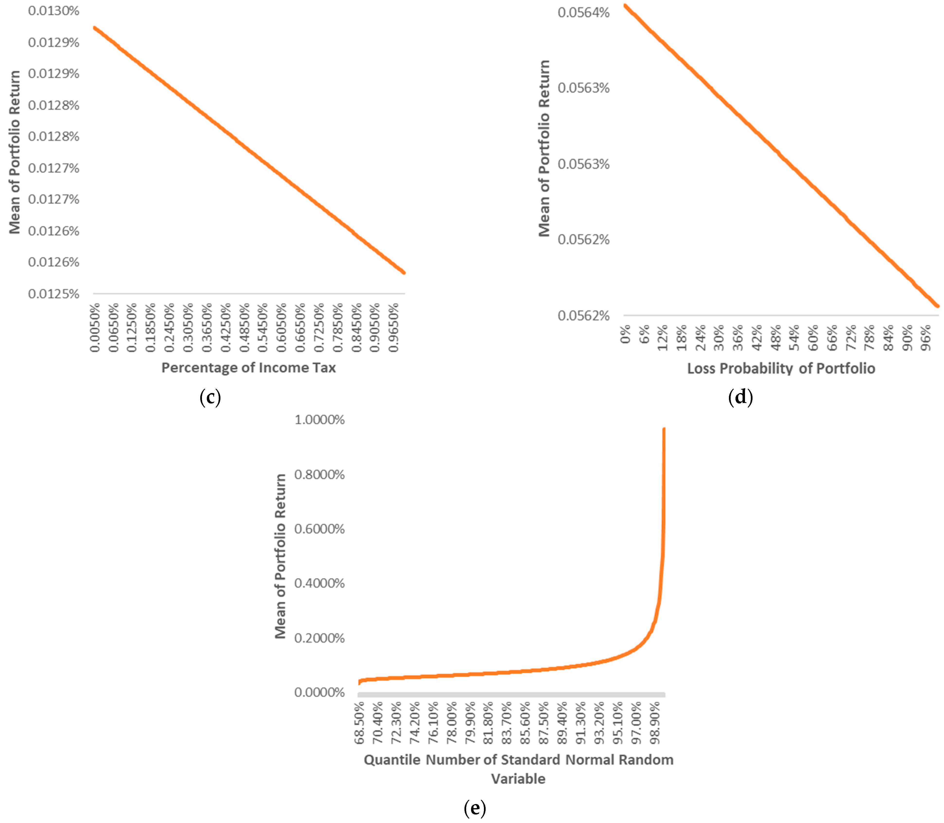MACD was chosen for its ability to provide clear buy or sell signals through the intersection of the MACD line and the signal line, allowing investors to identify optimal points to enter or exit the market quickly [42]. Finally, the portfolio’s mechanism for weighting stock capital uses the mean value at risk (mean VaR) model involving transaction cost and income tax variables. The mean-VaR model was chosen because it can adjust investors’ courage in bearing risk by choosing return quantiles in the VaR calculation [43]. This research academically develops a portfolio design mechanism by clustering stocks and analyzing its price movement trends, enabling investors to practically diversify and choose stocks with increasing price trends, reducing losses, and increasing profit opportunities.

2. Model Framework for the Selection and Capital Weighting of Stocks

2.1. Algorithm

The mechanism algorithm is given first to make it easier to follow the more detailed explanation in the following subsections. The algorithm of the mechanism is given in Figure 1. In writing, the following is an explanation of Figure 1:

(a)

Price data for stocks is input first.

(b)

Stocks are selected first based on their mean return value. Stocks with a positive mean of return are selected.

(c)

Stocks with a positive return mean are analyzed for buying indications using MACD. If the stock has a buy indication currently, the stock is selected to enter the next stage.

(d)

Each stock that has passed stage (c) is clustered using the K-means method based on its attributes: the mean and VaR of returns.

(e)

The best stocks from each cluster are selected to be designed into the portfolio. It is the final stock selection stage.

(f)

Each share in the portfolio is weighted by capital. Weighting is carried out using the mean-VaR model.

Figure 1. Algorithm for selection and capital weighting of stocks in a portfolio design.

Figure 1. Algorithm for selection and capital weighting of stocks in a portfolio design.

2.2. Mathematical Notations

The mathematical notations for the designed mechanism are defined first as follows:

(a)

$W$ represents the amount of capital in the portfolio in currency units. In this study, $W$ is assumed to be one to facilitate modeling.

(b)

$M$ represents the number of stocks selected at the beginning.

(c)

$P_{m,t}$ represents the price of the $m$-th stock at time $t$, where $m\in \left\{1,2,\dots , M\right\}$ and $t\in \left[0,\infty \right)$.

(d)

$N$ represents the number of stocks with a current buy indication that will be clustered later.

(e)

$P$ represents the number of attributes of the stock used in clustering. In this case, because two stock attributes are used, namely mean and value at risk of return, the $P$ value is two.

(f)

${\mu }_n$ represents the mean of return of the $n$-th stock, where $n\in \left\{1,2,\dots , N\right\}$.

(g)

$Va{R}_n$ represents the value at risk of return of the $n$-th stock, where $n\in \left\{1,2,\dots ,N\right\}$.

(h)

${\sigma }_{n_1,n_2}^2$ represents the covariance of returns from the $n_1$-th and $n_2$-th stocks, where $n_1,n_2\in \left\{1,2,\dots ,N\right\}$

(i)

$a_n$ represents a vector of size two containing the mean and value at risk of return of the $n$-th stock, where $n\in \left\{1,2,\dots , N\right\}$.

(j)

$K$ represents the number of clusters.

(k)

$v_k$ represents the centroid of the kth cluster, where $k\in \left\{1,2,\dots ,K\right\}.$

(l)

$S$ represents the final number of stocks selected in the portfolio.

(m)

$w_s$ represents the capital weight of the $s$-th stock in the portfolio, where $s\in \left\{1,2,\dots , S\right\}$.

2.3. Stock Selection Using MACD

Moving average convergence–divergence (MACD) is a tool for checking indications of when to buy or sell stocks. It can provide clear buy or sell signals through the intersection of the MACD line and the signal line, allowing investors to identify optimal points to enter or exit the market quickly [42].

The MACD value is calculated by subtracting the exponential moving average (EMA) value of order $p$ from the EMA value of order $q$ of the stock price, where $p$ and $q$ represent the number of trading days for one month and two weeks, respectively. The MACD value is then compared with the signal value, which is the EMA value of order $r$ of the MACD value, where $r$ represents the number of trading days for 1.5 weeks. Mathematically, the MACD value at time $\left(t+1\right)$ is expressed as follows [44]:

$$\mathrm{MACD}\left(t+1\right)={\mathrm{EMA}}_p\left(t+1\right)-{\mathrm{EMA}}_p\left(t+1\right),$$

(1)

where

$${\mathrm{EMA}}_p\left(t+1\right)=\frac{2}{p+1} P_{m,t}+\left(1-\frac{2}{p+1}\right){ \mathrm{EMA}}_p\left(t\right),$$

(2)

and

$${\mathrm{EMA}}_q\left(t+1\right)=\frac{2}{q+1} P_{m,t}+\left(1-\frac{2}{q+1}\right){\mathrm{EMA}}_q\left(t\right).$$

(3)

In more detail, $P_{m,t}$ represents the price of $m$-th stock at time $t$. Then, the signal line at time $\left(t+1\right)$ is mathematically expressed as follows [44]:

$$Si{g}_r\left(t+1\right)=\frac{2}{r+1}\mathrm{MACD}\left(t\right)+\left(1-\frac{2}{r+1}\right)Si{g}_r\left(t\right).$$

(4)

To start the calculation, the initial EMA value is given as the initial value of the actual data, and the initial signal value is the initial MACD value. In other words,

$${\mathrm{EMA}}_p\left(1\right)={\mathrm{EMA}}_p\left(1\right)=P_{m,1}$$

and

$$Si{g}_r\left(1\right)=\mathrm{MACD}\left(1\right).$$

The use of MACD in determining buy and sell times is as follows [45]:

(a)

Buy time is indicated when $\mathrm{MACD}\left(t\right)>Si{g}_r\left(t\right)$. This condition represents that stock prices tend to rise, so demand for them also rises.

(b)

Sell time is indicated when $\mathrm{MACD}\left(t\right)\le Si{g}_r\left(t\right)$. This condition represents that stock prices tend to fall, so demand for them also falls.

2.4. Stock Clustering Using the K-Means Method

The K-means method is a data clustering method with fast iteration speed, timely efficiency, and simple ability to provide a clear and well-defined cluster solution to help investors understand the relationship patterns between stocks in a portfolio [41]. The method is based on the shortest distance between data attributes and cluster centroids. This distance can be calculated using certain norms. Norm 2, better known as Euclidean distance, is the most popular because it is intuitive [46]. In summary, a cluster of data is the cluster with the smallest distance between the data and its centroid. The algorithm of this method is given in more detail in Figure 2.

Based on Figure 2, the K-means method is iterative. In the first iteration, the number of clusters and their centroids are determined first. Practically, a lot can be determined by visualizing the data in a scatter plot. Then, determining many clusters can be conducted using several methods, such as the elbow, silhouette, and gap statistics methods. Then, members of the clusters are data with the smallest distance between the attribute and the cluster centroid [47]. Once the clusters are filled with data, new centroids are determined. The new centroid of a cluster is the average value of each attribute in it. After that, the second iteration was carried out by returning to the stage of determining the members of each cluster. An iteration is stopped if the members of each cluster from the current iteration are the same as the members of each cluster in the previous iteration [48].

There are two stock attributes used in clustering in this research. These two are the mean and VaR of returns, each of which produces the following [49]:

$${\mu }_m=\frac{1}{T}{\displaystyle \sum }_{t=1}^T{R}_{m,t}$$

(5)

and

$${\mathrm{VaR}}_m=-\left[{\mu }_m+z_{\alpha }\frac{1}{T}{\displaystyle \sum }_{t=1}^T{\left(R_{m,t}-{\mu }_m\right)}^2\right],$$

(6)

where $T$ is the period considered, $R_{m,t}$ is the price of the $m$-th stock at time $t$, and $z_{\alpha }$ is the $\left(1-\alpha \right)$-th quantile of the standard normal cumulative distribution function.

2.5. Capital Weighing of Each Stock in Portfolios Using the Mean-VaR Model

The capital weighing model in investment portfolios generally applies the primary objectives of maximizing profits and minimizing losses. The mean of returns from the portfolio generally represents the profits from a portfolio. Then, there are several ways to represent losses from a portfolio. The first is the general one, where the negative value of the variance of returns represents losses. It is as introduced by Markowitz [24]. Second, losses can be represented by value at risk (VaR). VaR is the maximum loss tolerated by investors. VaR is considered more flexible than the variance of return because there is a tolerance for accepting losses from the investors involved [50]. This model with VaR is usually called the mean-VaR model.

Suppose a stock portfolio containing $S$ stocks have total capital $W$ in currency units. For practical reasons in modeling, the value of $W$ is assumed to be one. Then, suppose that the capital weight of each stock is $w_s$ and the return is $R_S$ with $s\in \left\{1,2,\dots , S\right\}$. For each $s$, $R_s$ is assumed to be a normal random variable with mean ${\mu }_s$ and variance ${\sigma }_s^2$. Verbally, this assumption indicates that stock returns are independent of time because the mean and variance are constant. It can also be said that there is no jumping in the return. In other words, situations such as pandemics and chaos in the economic situation have not been resolved using this mechanism [51].

The return from a portfolio is defined as the sum of the multiplication of each stock weight and its return. Mathematically, this is defined as follows:

$${\mathcal{R}}_S={\displaystyle \sum }_{s=1}^S{w}_s{R}_s,$$

Costs must be incurred when buying and selling stocks. These costs are called transaction costs. The transaction cost for buying stocks in a portfolio is a percentage of the total buy transaction amount. The percentage of each stock-buying transaction cost is assumed to be the same. Mathematically, this is expressed as follows:

$${\mathcal{T}}_{S,B}=\eta ,$$

where $\eta$ is the transaction cost percentage of buying stocks. Then, the transaction costs for selling stocks from the portfolio are a percentage of the total selling transactions. The percentage of each stock-selling transaction cost is assumed to be the same. Mathematically, this is expressed as follows:

$${\mathcal{T}}_{S,\mathcal{S}}=\theta \left(1+{\displaystyle \sum }_{s=1}^S{w}_s{R}_s\right),$$

where $\theta$ is the transaction cost percentage of selling stocks. Thus, the total transaction costs for buying and selling stocks in the portfolio are as follows:

$${\mathcal{T}}_S={\mathcal{T}}_{S,B}+{\mathcal{T}}_{S,\mathcal{S}}=\eta +\theta \left(1+{\displaystyle \sum }_{s=1}^S{w}_s{R}_s\right).$$

Then, when the stocks in the portfolio are sold, there is also income tax that must be paid. This tax is paid if the return from the portfolio is nonnegative. Mathematically, this is expressed as follows:

$$T_S=\left\{\begin{array}{cc}\zeta {\displaystyle {\displaystyle \sum }_{s=1}^S}{w}_s{R}_s& ;{\displaystyle {\displaystyle \sum }_{s=1}^S}{w}_s{R}_s>0\\ 0& ;{\displaystyle {\displaystyle \sum }_{s=1}^S}{w}_s{R}_s\le 0\end{array}\right.,$$

where $\zeta$ is the income tax percentage. Thus, the portfolio return that has been reduced by transaction costs and income tax is as follows:

$${\Re }_S={\mathcal{R}}_S-{\mathcal{T}}_S-T_S.$$

(7)

Next, the mean of return of portfolio $P$ is calculated as the expectation of ${\Re }_S$. Mathematically, this is given in the following equation:

$${\mu }_P=E\left({\Re }_S\right)=E\left({\mathcal{R}}_S-{\mathcal{T}}_S-T_S\right)={\displaystyle \sum }_{s=1}^S{w}_s{\mu }_s\left[1-\theta -\zeta +\zeta \mathrm{Pr}\left({\displaystyle \sum }_{s=1}^S{w}_s{R}_s\le 0\right)\right]-\eta .$$

(8)

In detail, $\sum _{s=1}^S{w}_s{R}_s~N\left[\sum _{s=1}^S{w}_s{\mu }_s,\sum _{s=1}^S{\left(w_s{\sigma }_s\right)}^2\right]$. Thus,

$$\mathrm{Pr}\left({\displaystyle \sum }_{s=1}^S{w}_s{R}_s\le 0\right)=\frac{1}{\sqrt{2\pi {\sum }_{s=1}^S{\left(w_s{\sigma }_s\right)}^2}}{{\displaystyle \int }}_{-\infty }^0{e}^{-\frac{1{\left(x-{\sum }_{s=1}^S{w}_s{\mu }_s\right)}^2}{2{\sum }_{s=1}^S{\left(w_s{\sigma }_s\right)}^2}}dx.$$

(9)

Using Equation (9) to determine the maximum value of the mean of portfolio return in Equation (8) has complications. Therefore, the approach from Equation (9) can be used as an alternative. One such approach is the approximation method of Bowling et al. [52] as follows:

$$\mathrm{Pr}\left({\displaystyle \sum }_{s=1}^S{w}_s{R}_s\le 0\right)\approx \frac{1}{1+e^{1.702\left(\frac{{\sum }_{s=1}^S{w}_s{\mu }_s}{\sqrt{{\sum }_{s=1}^S{\left(w_s{\sigma }_s\right)}^2}}\right)}}.$$

(10)

Thus, Equation (8) can be rewritten as follows:

$${\mu }_P={\displaystyle \sum }_{s=1}^S{w}_s{\mu }_s\left[1-\theta -\zeta +\zeta \frac{1}{1+e^{1.702\left(\frac{{\sum }_{s=1}^S{w}_s{\mu }_s}{\sqrt{{\sum }_{s=1}^S{\left(w_s{\sigma }_s\right)}^2}}\right)}}\right]-\eta .$$

(11)

For reasons of simplicity in modeling, we assume that $\mathit{Pr}\left({\sum }_{s=1}^S{w}_s{R}_s\le 0\right)=0.5$. Thus, Equation (11) can be rewritten as follows:

$${\mu }_P=\left(1-\theta -0.5\zeta \right){\displaystyle \sum }_{s=1}^S{w}_s{\mu }_s-\eta -\theta .$$

(12)

Equation (12) can be written in the form of matrix and vector multiplication as follows:

$${\mu }_P=\left(1-\theta -0.5\zeta \right)w^T\mu -\eta -\theta .$$

(13)

where

$$w=\left[\begin{array}{c}{w}_1\\ w_2\\ ⋮\\ w_S\end{array}\right] \mathrm{and} \mu =\left[\begin{array}{c}{\mu }_1\\ {\mu }_2\\ ⋮\\ {\mu }_S\end{array}\right].$$

Then, the VaR of portfolio returns at level $\left(1-\alpha \right)$ can be expressed as follows:

$$\begin{gathered} {\mathrm{VaR}}_P=E\left\{-\left[{\displaystyle \sum }_{s=1}^S{w}_s{R}_s+z_{\alpha }\sqrt{{\displaystyle \sum }_{s=1}^S{\displaystyle \sum }_{k=1}^S{w}_s{w}_k\left(R_s-{\mu }_s\right)\left(R_k-{\mu }_k\right)}\right]\right\}, \\ =-\left\{{\displaystyle \sum }_{s=1}^S{w}_{s}E\left(R_s\right)+z_{\alpha }\sqrt{{\displaystyle \sum }_{s=1}^S{\displaystyle \sum }_{k=1}^S{w}_s{w}_{k}E\left[\left(R_s-{\mu }_s\right)\left(R_k-{\mu }_k\right)\right]}\right\}, \\ =-\left({\displaystyle \sum }_{s=1}^S{w}_s{\mu }_s+z_{\alpha }\sqrt{{\displaystyle \sum }_{s=1}^S{\displaystyle \sum }_{k=1}^S{w}_s{w}_k{\sigma }_{sk}}\right), \end{gathered}$$

(14)

where $z_{\alpha }$ represents the $\left(1-\alpha \right)$-th quantile of a standard normal distribution random variable, and ${\sigma }_{sk}$ with $s,k\in \left\{1,2,\dots , S\right\}$ is the covariance between the $s$-th and $k$-th stock returns. Equation (14) can also be expressed as matrix multiplication. The expression is as follows:

$${\mathrm{VaR}}_P=-\left(w^T\mu +z_{\alpha }\sqrt{w^T\Sigma w}\right),$$

(15)

where $\Sigma =\left[{\sigma }_{sk}\right]\in {ℝ}^{S\times S}$.

In a typical capital weighing problem, the constraint function is usually the total sum of the weights. The sum of the capital weights of all stocks is one. It is mathematically expressed as follows:

$${\displaystyle \sum }_{s=1}^S{w}_s=1,$$

(16)

or

$$w^{T}e=1,$$

(17)

where

$$e=\left[\begin{array}{c}1\\ 1\\ ⋮\\ 1\end{array}\right].$$

Thus, the problem of maximizing the mean of portfolio return and minimizing the VaR of portfolio return can be formulated as follows:

$$\begin{gathered} \max . 2\tau {\mu }_P+{\mathrm{VaR}}_P=2\tau \left[\left(1-\theta -0.5\zeta \right)w^T\mu -\eta -\theta \right]-w^T\mu -z_{\alpha }\sqrt{w^T\Sigma w} \\ \mathrm{s}.\mathrm{t}. w^{T}e=1, w\ge 0 \end{gathered}$$

(18)

The $\tau$ value in Equation (18) represents the risk tolerance coefficient of investors. The smaller the value of the coefficient, the smaller the loss tolerated, and vice versa. In simple terms, if investors tolerate a small risk of loss, then the expected loss is also slight, and vice versa.

The solution of the mean-VaR model in Equation (18) can be determined using the Lagrange multiplier method. Through this method, the optimization model in Equation (18) is converted into an optimization model without constraint functions as follows:

$$\max . \mathcal{L}\left(w,\lambda \right)=2\tau \left[\left(1-\theta -0.5\zeta \right)w^T\mu -\eta -\theta \right]-z_{\alpha }\sqrt{w^T\Sigma w}+\lambda \left(w^{T}e-1\right),$$

(19)

where $\lambda$ is positive Lagrange multiplier, and $w\ge \mathbf{0}$. $w$ and $\lambda$ estimators are solutions of the following equations:

$$\frac{\partial }{\partial w}\mathcal{L}\left(w,\lambda \right)=2\tau \left(1-\theta -0.5\zeta \right)\mu -\mu -z_{\alpha }\frac{\Sigma w}{\sqrt{w^T\Sigma w}}+\lambda e=\mathbf{0},$$

(20)

and

$$\frac{\partial }{\partial \lambda }\mathcal{L}\left(w,\lambda \right)=w^{T}e-1=0.$$

(21)

Briefly, the solution of Equation (18) is as follows:

$$w=\frac{{\Sigma }^{-1}\left\{\left[2\tau \left(1-\theta -0.5\zeta \right)-1\right]\mu +\lambda e\right\}}{e^T{\Sigma }^{-1}\left\{\left[2\tau \left(1-\theta -0.5\zeta \right)-1\right]\mu +\lambda e\right\}}.$$

(22)

In detail,

$$\lambda =\frac{-b\pm \sqrt{b^2-4ac}}{2a},$$

(23)

where $a=e^T{\Sigma }^{-1}e$, $b=2\left[2\tau \left(1-\theta -0.5\zeta \right)-1\right]e^T{\Sigma }^{-1}\mu$, and $c={\left[2\tau \left(1-\theta -0.5\zeta \right)-1\right]}^2{\mu }^T{\Sigma }^{-1}\mu -z_{\alpha }^2$. Note that the value of $\tau$ must cause $w\ge 0$ dan $\lambda >0$.

3. Mechanism Application to Real Data

3.1. Description of Data Used

In applying the mechanisms to real data, we consider Indonesia a member of G20 countries, with the third most significant economic growth within it in the third quarter of 2023, after China and India. The stability and management of inflation, interest rates, and political events in 2023 are reassuring [53]. We utilize the finest capital market statistics for 2022 Southeast Asia, specifically the Indonesian Stock Exchange (BEI) [54]. The data provided are stock return data specifically for the Kompas 100 Index in Indonesia. The Kompas 100 Index comprises 100 stocks with the highest liquidity, most significant market capitalization value, vital fundamentals, and best performance in the Indonesian stock market. The determination of the 100 stocks is valid from August 2023 to January 2024. The mechanism can not only be used on Indonesian data, but in this case, we chose Indonesia because it has the best capital market in Southeast Asia, the region with the fastest economic growth worldwide in 2022. Then, the period considered is from 9 October 2022 to 9 October 2023. Data were obtained from the website https://yahoo.finance accessed on 9 October 2023 and summarized in the following link: https://bit.ly/100IndexStockDataIndonesia (accessed on 9 October 2023). These stocks are listed in

Table 1. List of stock codes in each sector on the 100 Kompas Index in Indonesia.

Sector	Frequency	Stock Code
Financials	16	AGRO, ARTO, BBCA, BBKP, BBNI, BBRI, BBTN, BDMN, BFIN, BMRI, BRIS, BTPS, PNBN, PNIN, PNLF, STRG
Energy	15	ADMR, ADRO, AKRA, DOID, ELSA, ENRG, BSSR, HRUM, INDY, ITMG, MEDC, PGAS, PTBA, RAJA, RMKE
Basic Materials	14	AGII, ANTM, AVIA, BRMS, BRPT, ESSA, INCO, INKP, INTP, MDKA, SMGR, TINS, TKIM, TPIA
Primary Consumer Goods	14	AALI, AMRT, CPIN, DSNG, GGRM, HMSP, ICBP, INDF, JPFA, LSIP, MYOR, SSMS, TAPG, UNVR
Infrastructures	11	ADHI, EXCL, ISAT, JKON, JSMR, MTEL, PTPP, TBIG, TLKM, TOWR, WIKA
Nonprimary Consumer Goods	8	ACES, ERAA, LPPF, MAPI, MNCN, MPMX, MSIN, SCMA
Healthcare	7	HEAL, KLBF, MIKA, MMIX, MTMH, OMED, SIDO
Industrials	5	ABMM, ASII, BMTR, EMTK, UNTR
Properties and Real Estate	4	BSDE, CTRA, PWON, SMRA
Technology	4	BELI, BUKA, GOTO, WIFI
Transportation and Logistics	2	ASSA, SMDR
Total	100

below based on their sector.

Table 1 shows that the sector with the most significant number of stocks in the 100 index is financial. In other words, the financial sector in Indonesia has the most considerable liquidity and capitalization among other sectors. Then, in second place is the energy sector, where the number of stocks differs from one with finance, namely 15. Meanwhile, the sector with the fewest stocks is the transportation and logistics sector, which has only two stocks. In other words, this sector has the smallest liquidity and capitalization among all sectors.

3.2. Clustered Data Selection

The data to be clustered are selected first. There are two stages of selection. The first selection is the selection of the mean return value of the stocks. Stocks with a positive mean of return are selected. After the examination, 40 out of 100 stocks had a positive mean of return, as shown in Figure 3, where the abscissa shows the alphabetical order of the stocks and the ordinate shows the mean of returns of the stocks. The 40 stocks were then selected in stage two. In stage two, stocks are selected based on buy indicators based on the MACD indicator. The p, q, and r orders used are 12, 26, and 9. These order values are the best in terms of statistical error. Stocks that have buy indications are selected. Of the 40 shares, there are 18 that have buy indications, as given in

Table 2. Checking buy indications on 40 stocks in the Kompas 100 Index with a positive mean of return using MACD.

Stock Code	$\mathbf{MACD}\mathbf{\left(}\mathit{t}\mathbf{\right)}$	$\mathit{S}\mathit{i}{\mathit{g}}_{\mathit{r}}\mathbf{\left(}\mathit{t}\mathbf{\right)}$	Does the Stock Have a Buy Indication?
ABMM	−19.60	−1.39	No
ACES	6.68	10.07	No
AKRA	9.48	19.36	No
AMRT	−8.93	11.93	No
BBCA	−26.36	−39.07	Yes
BBNI	143.26	124.69	Yes
BBRI	−86.91	−75.08	No
BELI	−0.28	−0.37	Yes
BFIN	−36.64	−33.46	No
BMRI	37.18	48.76	No
BRIS	−31.41	−21.16	No
BRMS	−2.81	2.80	No
BRPT	53.76	89.07	No
BSDE	−13.41	−20.68	Yes
CPIN	134.62	59.03	Yes
CTRA	−19.13	−21.58	Yes
DOID	27.81	22.70	Yes
DSNG	5.32	4.43	Yes
ELSA	−2.23	2.06	No
ENRG	−1.68	3.20	No
ERAA	−14.68	−12.09	No
EXCL	5.39	10.70	No
GGRM	15.24	−127.52	Yes
HRUM	6.39	36.78	No
ICBP	15.88	−29.46	Yes
INDF	−35.69	−71.16	Yes
INKP	160.60	352.62	No
INTP	−191.78	−186.63	No
ISAT	206.66	157.69	Yes
JSMR	14.22	60.31	No
MAPI	11.77	−11.27	Yes
MEDC	39.77	88.66	No
MIKA	−10.58	−20.79	Yes
MPMX	−4.14	−3.26	No
MYOR	16.98	−1.11	Yes
RAJA	−1.88	9.60	No
SMRA	−16.79	−17.73	Yes
SSMS	15.53	6.84	Yes
TKIM	193.69	429.13	No
TPIA	126.52	122.84	Yes

. These 18 stocks are then clustered using the K-means method.

3.3. Data Clusterization and Stock Selection

Based on the data selection results, a description of the data to be clustered is given in

Table 3. Description of 18 data to be clustered.

Stock Code	Sector	Mean of Return	VaR of Return
MAPI	Non-primary Consumer Goods	$2.952\times {10}^{-3}$	$-5.010\times {10}^{-2}$
CPIN	Primary Consumer Goods	$4.287\times {10}^{-4}$	$-3.008\times {10}^{-2}$
DSNG	Primary Consumer Goods	$8.042\times {10}^{-4}$	$-3.813\times {10}^{-2}$
GGRM	Primary Consumer Goods	$1.775\times {10}^{-3}$	$-4.266\times {10}^{-2}$
ICBP	Primary Consumer Goods	$3.986\times {10}^{-4}$	$-2.195\times {10}^{-2}$
INDF	Primary Consumer Goods	$2.754\times {10}^{-4}$	$-2.106\times {10}^{-2}$
MYOR	Primary Consumer Goods	$8.772\times {10}^{-4}$	$-3.543\times {10}^{-2}$
SSMS	Primary Consumer Goods	$6.665\times {10}^{-4}$	$-5.099\times {10}^{-2}$
TPIA	Basic Materials	$5.550\times {10}^{-4}$	$-3.055\times {10}^{-2}$
DOID	Energy	$1.953\times {10}^{-3}$	$-4.328\times {10}^{-2}$
BBCA	Financials	$1.983\times {10}^{-4}$	$-1.906\times {10}^{-2}$
BBNI	Financials	$2.829\times {10}^{-4}$	$-2.296\times {10}^{-2}$
MIKA	Healthcare	$1.313\times {10}^{-3}$	$-4.265\times {10}^{-2}$
ISAT	Infrastructures	$1.092\times {10}^{-3}$	$-3.466\times {10}^{-2}$
BSDE	Properties and Real Estate	$7.175\times {10}^{-4}$	$-2.794\times {10}^{-2}$
CTRA	Properties and Real Estate	$5.164\times {10}^{-4}$	$-2.996\times {10}^{-2}$
SMRA	Properties and Real Estate	$7.272\times {10}^{-4}$	$-3.602\times {10}^{-2}$
BELI	Technology	$6.019\times {10}^{-5}$	$-1.494\times {10}^{-2}$

. Table 3 shows that the 18 stocks to be clustered come from nine sectors: Non-primary Consumer Goods, Primary Consumer Goods, Basic Materials, Energy, Financials, Healthcare, Infrastructures, Properties and Real Estate, and Technology. There are no stocks from two sectors: Industrials and Transportation and Logistics. The Primary Consumer Goods sector stocks are the most numerous, with seven stocks. Then, the Energy, Basic Materials, Healthcare, Infrastructures, and Technology sectors each have one stock. Of the stocks to be clustered, the stock with the most significant mean of return is MAPI. MAPI also has the largest VaR of return. Then, SSMS and BELI each have the most minor mean of return and VaR of return.

Many clusters are determined first using the silhouette method. The practice is carried out using the help of R Studio software version 4.1.2 with the package “factoextra” and the function “fviz_nbclust(data, K-means, method = ‘silhouette’)”. The number of clusters selected is the one with the most significant average silhouette [55]. Briefly, the results of determining these many clusters are given visually in Figure 4.

Figure 4 shows that the most significant average silhouette width value occurs when the number of clusters is five. Therefore, the number of clusters selected based on these results is five. Next is determining the members of each cluster. This determination was carried out using the K-means method, as explained in Section 2.4. Cluster determination was carried out one hundred times to measure the accuracy of the clusterization results. The results of one hundred clusterization experiments are given in

Table 4. Results of one hundred experiments in determining clusters from 18 stocks.

Stock Code	Frequency of Appearance in Clusters					Chosen Cluster	Accuracy (%)
	1	2	3	4	5
MAPI	100	-	-	-	-	1	100
DOID	81	19	-	-	-	1	81
GGRM	100	-	-	-	-	1	100
MIKA	83	17	-	-	-	1	83
SSMS	100	-	-	-	-	1	100
MYOR	9	81	10	-	-	2	81
DSNG	-	85	11	4	-	2	85
ISAT	-	89	11	-	-	2	89
SMRA	-	95	5	-	-	2	95
TPIA	-	-	68	25	7	3	68
CTRA	-	-	73	27	-	3	73
CPIN	-	-	70	30	-	3	70
BSDE	-	-	6	67	27	4	67
ICBP	-	-	5	29	66	5	66
INDF	-	-	2	14	84	5	84
BBNI	-	-	5	27	68	5	68
BBCA	-	-	-	31	69	5	69
BELI	-	-	-	33	67	5	67
Average of Accuracy (%)							80.33

.

Table 4 shows that the average accuracy of the clusterization results of the data using the K-means method is 80.33%. This accuracy value is high. Hence, the results can be said to be accurate [56]. A summary of the results for the members and centroids of each cluster is given in

Table 5. The final results of the five stock clusters.

Cluster	Centroid	Member of Cluster
1	$\left[\begin{array}{c}1.145\times {10}^{-3}\\ -4.594\times {10}^{-2}\end{array}\right]$	MAPI, GGRM, SSMS, DOID, MIKA
2	$\left[\begin{array}{c}1.139\times {10}^{-3}\\ -3.606\times {10}^{-2}\end{array}\right]$	DSNG, MYOR, ISAT, SMRA
3	$\left[\begin{array}{c}4.069\times {10}^{-4}\\ -3.019\times {10}^{-2}\end{array}\right]$	CPIN, TPIA, CTRA
4	$\left[\begin{array}{c}7.272\times {10}^{-4}\\ -2.794\times {10}^{-2}\end{array}\right]$	BSDE
5	$\left[\begin{array}{c}5.390\times {10}^{-4}\\ -1.999\times {10}^{-2}\end{array}\right]$	ICBP, INDF, BBCA, BBNI, BELI

.

The next step after the stock cluster is obtained is stock selection in preparing the final portfolio. The number of stocks selected is five, with one selected from each cluster. The stocks selected in a cluster have the most significant Sharpe ratio [57]. A list of Sharpe ratios for each stock in each cluster is given in

Table 6. List of Sharpe ratios of each stock in each cluster.

Cluster	Stock Code	Sharpe Ratio
1	MAPI	$1.030\times {10}^{-1}$
	DOID	$9.821\times {10}^{-2}$
	GGRM	$7.033\times {10}^{-2}$
	MIKA	$6.331\times {10}^{-2}$
	SSMS	$2.150\times {10}^{-5}$
2	MYOR	$6.847\times {10}^{-2}$
	DSNG	$5.971\times {10}^{-2}$
	ISAT	$4.849\times {10}^{-2}$
	SMRA	$4.395\times {10}^{-2}$
3	TPIA	$4.452\times {10}^{-2}$
	CTRA	$2.828\times {10}^{-2}$
	CPIN	$2.388\times {10}^{-2}$
4	BSDE	$2.814\times {10}^{-2}$
5	ICBP	$3.513\times {10}^{-2}$
	INDF	$1.520\times {10}^{-2}$
	BBNI	$1.098\times {10}^{-2}$
	BBCA	$9.105\times {10}^{-3}$
	BELI	$6.655\times {10}^{-3}$

. Based on Table 6, the stocks with the most significant Sharpe ratios from each cluster are MAPI, MYOR, TPIA, BSDE, and ICBP. Therefore, these stocks were chosen for the investment portfolio in this research. The five stocks come from four sectors, namely primary consumer goods, properties and real estate, basic materials, and non-primary consumer goods. MYOR and ICBP are in the same sector, while others differ. It means that the method used for selecting stocks in the portfolio in this research can be used for diversification. Statistically, this can be seen from the correlation between stock returns in the correlation matrix $\Omega$ in Equation (24), where the values are small. In fact, some have negative values.

$$\Omega =\left[\begin{array}{ccccc}1& 1.149\times {10}^{-1}& -4.947\times {10}^{-2}& -3.438\times {10}^{-4}& 2.272\times {10}^{-2}\\ 1.149\times {10}^{-1}& 1& -4.942\times {10}^{-2}& 9.655\times {10}^{-2}& 2.368\times {10}^{-1}\\ -4.947\times {10}^{-2}& -4.942\times {10}^{-2}& 1& 3.192\times {10}^{-2}& 7.290\times {10}^{-2}\\ -3.438\times {10}^{-4}& 9.655\times {10}^{-2}& 3.192\times {10}^{-2}& 1& -9.975\times {10}^{-2}\\ 2.272\times {10}^{-2}& 2.368\times {10}^{-1}& 7.290\times {10}^{-2}& -9.975\times {10}^{-2}& 1\end{array}\right].$$

(24)

3.4. Capital Weighing

At the beginning of this stage, we first determine $\mu$ and $\Sigma$ from the data obtained. Briefly, the results are given in the following equations:

$$\mu =\left[\begin{array}{c}2.952\times {10}^{-3}\\ 1.313\times {10}^{-3}\\ 5.164\times {10}^{-4}\\ 7.272\times {10}^{-4}\\ 8.772\times {10}^{-4}\end{array}\right],$$

(25)

and

$$\Sigma =\left[\begin{array}{ccccc}8.216\times {10}^{-4}& 6.832\times {10}^{-5}& -2.589\times {10}^{-5}& -1.631\times {10}^{-7}& 8.341\times {10}^{-6}\\ 6.832\times {10}^{-5}& 4.301\times {10}^{-4}& -1.871\times {10}^{-5}& 3.313\times {10}^{-5}& 6.291\times {10}^{-5}\\ -2.589\times {10}^{-5}& -1.871\times {10}^{-5}& 3.334\times {10}^{-4}& 9.643\times {10}^{-6}& 1.705\times {10}^{-5}\\ -1.631\times {10}^{-7}& 3.313\times {10}^{-5}& 9.643\times {10}^{-6}& 2.738\times {10}^{-4}& -2.115\times {10}^{-5}\\ 8.341\times {10}^{-6}& 6.291\times {10}^{-5}& 1.705\times {10}^{-5}& -2.115\times {10}^{-5}& 1.641\times {10}^{-4}\end{array}\right]$$

(26)

After that, we determine the percentages of buying transaction costs $\eta$ and selling transaction costs $\theta$ is 0.0.4%. Then, the income tax percentage $\zeta$ is 0.1%. Finally, the value of $\tau$ that causes the values $w_s\ge 0$ and $\lambda >0$ is sought. For the lambda value in Equation (23), we use $\frac{-b+\sqrt{b^2-4ac}}{2a}$ instead of $\frac{-b+\sqrt{b^2-4ac}}{2a}$ because this gives a value of $\lambda >0$. Briefly, after the search is performed, we obtain that the values $w_s\ge 0$ and $\lambda >0$ are satisfied when $0<\tau \le 5.112$. To select the most optimal weights, we use the Sharpe ratio measure. The weight that produces the most excellent Sharpe ratio is the one we choose. In short, it turns out that the optimal weight occurs when $\tau =5.112$. A summary of the results of determining optimal weights accompanied by descriptive statistics for the portfolio is given in

Table 7. Results of determining optimal weights accompanied by descriptive statistics from the portfolio.

Variable	Value
$\tau$	$5.112$
$\lambda$	$1.196\times {10}^{-6}$
$w_1$	$2.434\times {10}^{-1}$
$w_2$	$1.175\times {10}^{-1}$
$w_3$	$1.120\times {10}^{-1}$
$w_4$	$1.947\times {10}^{-1}$
$w_5$	$3.324\times {10}^{-1}$
${\displaystyle {\displaystyle \sum }_{s=1}^6}{w}_s$	$1$
Mean of Portfolio Return	$5.626\times {10}^{-4}$
Deviation Standard of Portfolio Return	$9.800\times {10}^{-3}$
Value at Risk of Portfolio Return	$-1.748\times {10}^{-2}$
Sharpe ratio	$5.741\times {10}^{-2}$

.

4. Discussion

4.1. Sensitivity Analyses

In this subsection, we first visually analyze the relationship between the mean and VaR of portfolio returns. The analysis was carried out on the interval $0<\tau \le 5.112$, obtained in Section 3.4. Briefly, the relationship between the mean and VaR of portfolio returns is given visually in Figure 5.

Figure 5 shows that the mean and VaR of portfolio returns have an in-line relationship. In other words, the greater the mean of portfolio return, the greater the VaR, and vice versa. It is logical because the more significant the loss we tolerate, the greater the return we will get, and vice versa.

Next, a sensitivity analysis of several variables involved in the mean and standard deviation of returns is carried out. The variables whose sensitivity analysis is analyzed are income tax, transaction tax, risk tolerance, $z_{\alpha }$ on VaR, and loss probability. When a variable is analyzed for sensitivity, the values of other variables are considered constant. Briefly, the sensitivity analysis results of the variables on the mean of portfolio return are given visually in Figure 6. Then, the sensitivity analysis results of the variables on the standard deviation are given in Figure 7.

Figure 6 shows that buying transaction costs, selling transaction costs, income taxes, and the probability for portfolio losses have no in-line relationship with the mean of portfolio return. In other words, the greater the value of the four, the smaller the mean of portfolio return, and vice versa. It makes sense because when all four exist, this will reduce the mean of portfolio returns. Then, the $z_{\alpha }$ value in the VaR calculation of portfolio returns appears to have an in-line relationship with the mean of portfolio returns. It also makes sense because the more significant the $z_{\alpha }$ value, the greater the VaR value of the portfolio return, and vice versa. In other words, it will also cause the mean of portfolio return to be more significant. It also applies vice versa.

Meanwhile, Figure 7 shows that selling transaction costs, income taxes, and the probability of portfolio loss have no in-line relationship with the standard deviation of portfolio returns. It means that the greater the value of the three, the smaller the value of the standard deviation of portfolio returns, and vice versa. Practically, it makes sense because when all three values exist, the mean of portfolio return will be small, so the standard deviation will also be slight. Then, the $z_{\alpha }$ value in the VaR calculation of portfolio returns appears to have an in-line relationship with the standard deviation of portfolio returns. It also makes sense because the more significant the $z_{\alpha }$ value, the greater the VaR of the portfolio return, and vice versa. In other words, this will also cause the standard deviation of portfolio returns to become more prominent. It also applies vice versa.

Finally, we analyze the influence of risk tolerance on the mean and VaR of portfolio returns. The analysis was carried out visually; the results are in Figure 8. Figure 8 shows that risk tolerance has an in-line relationship with the mean and VaR of portfolio returns. In other words, the greater the investor’s tolerance for loss, the greater the mean and VaR of portfolio return. It is logical. The results of the sensitivity analysis in this section all seem logical. It indicates that the capital selection and weighting mechanism can describe the actual situation.

4.2. Comparation with Another Mechanism

In this subsection, we will compare experimental data results using the first and second mechanisms. The first mechanism (MI) is the mechanism that was introduced. In contrast, the second mechanism (MII) is the mean-VaR mechanism without the involvement of clusterization and analysis of stock price movements. The experimental results that are compared are the mean of portfolio returns from each mechanism. After that, each result of the mechanism is also compared with the actual reality the next day. Without clustering and analyzing stock price movements, we selected five stocks from the Kompas 100 Index with the most significant Sharpe ratios. MAPI, ISAT, BRPT, JSMR, and ICBP are the five stocks. Only two shares are the same from MI and MII, MAPI and ICBP. Briefly, the comparison results between the two mechanisms are given in

Table 8. Mean of portfolio return from two compared mechanisms and actual mean of portfolio return on the next day.

Mechanism	Mean of Portfolio Return	Real Mean of Portfolio Return
MI	$5.626\times {10}^{-4}$	$7.149\times {10}^{-4}$
MII	$1.889\times {10}^{-3}$	$-1.394\times {10}^{-3}$

.

Table 8 shows that the mean of portfolio return from MII is greater than MI. However, if the two mean portfolio returns are compared with the actual one the next day, the mean portfolio return from MI is achieved or even exceeds it. In contrast, the mean of portfolio return from MII is not achieved and is even negative. These results indicate that clustering and analysis of stock price movements should be carried out in forming a stock portfolio.

5. Conclusions

This research develops the stock selection and capital weighting mechanisms for portfolio design. The stock selection mechanism is based on clustering analysis and analysis of the timing of buying and selling stocks. Clustering is conducted to select stocks with different characteristics to diversify risks. Then, an analysis of buying and selling times is carried out to reduce the chance of a decline in stock prices in the short term, thereby reducing the chance of loss from the portfolio. Clustering was carried out using the K-means method. This method was chosen because it is suitable for grouping shares based on mean and VaR characteristics. This suitability can be seen from its application, where the accuracy of using this method is above eighty percent. Then, the time to buy and sell stocks is analyzed using the moving average convergence–divergence (MACD) indication. MACD can describe stock price movements better than other indications because it uses two indication lines at once, namely the MACD line and the signal line. Finally, the portfolio’s mechanism for weighting stock capital uses the mean value at risk (mean VaR) model involving transaction cost and income tax variables. The mean-VaR model was chosen because it can adjust investors’ courage in bearing risk by choosing return quantiles in the VaR calculation.

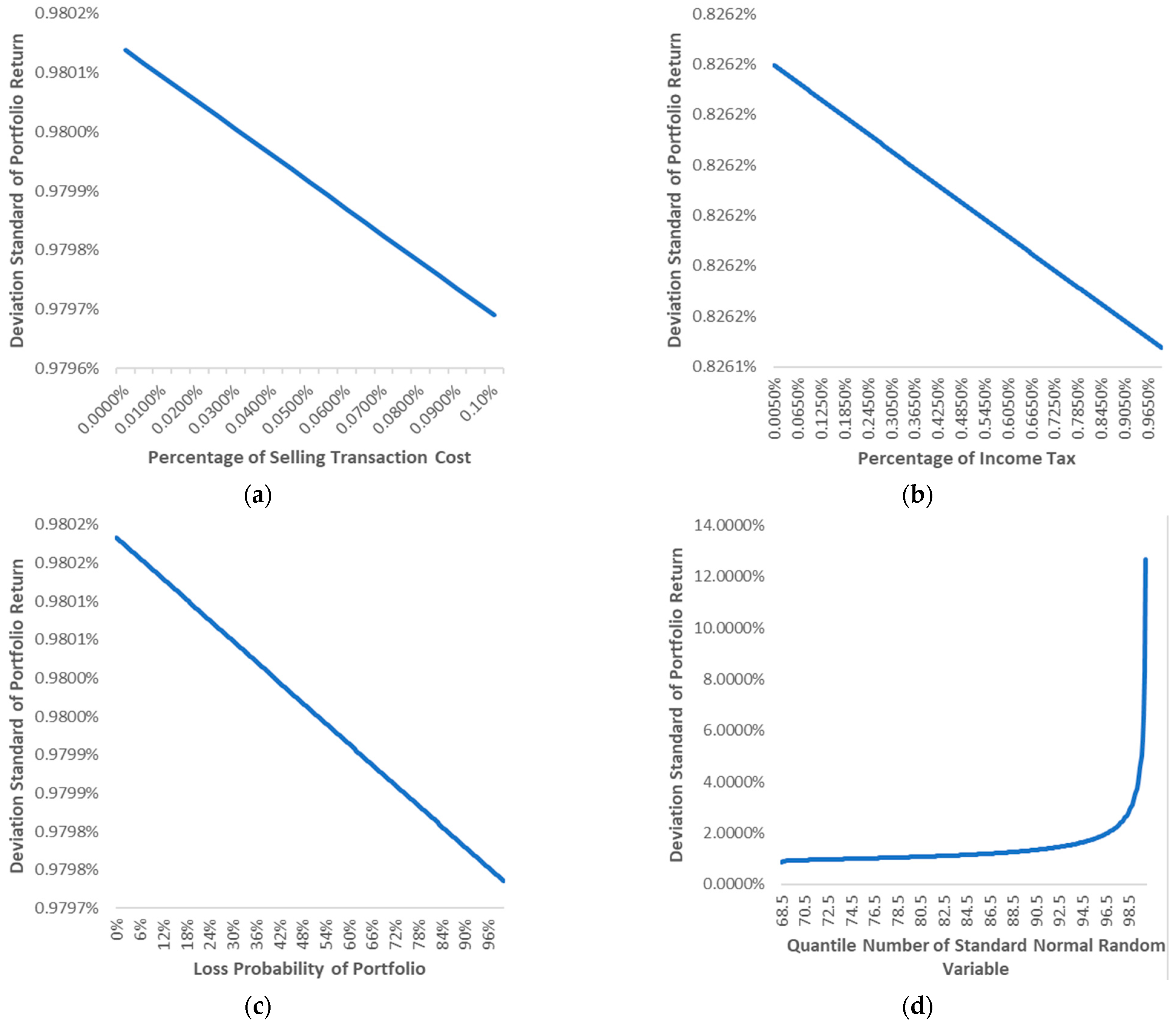
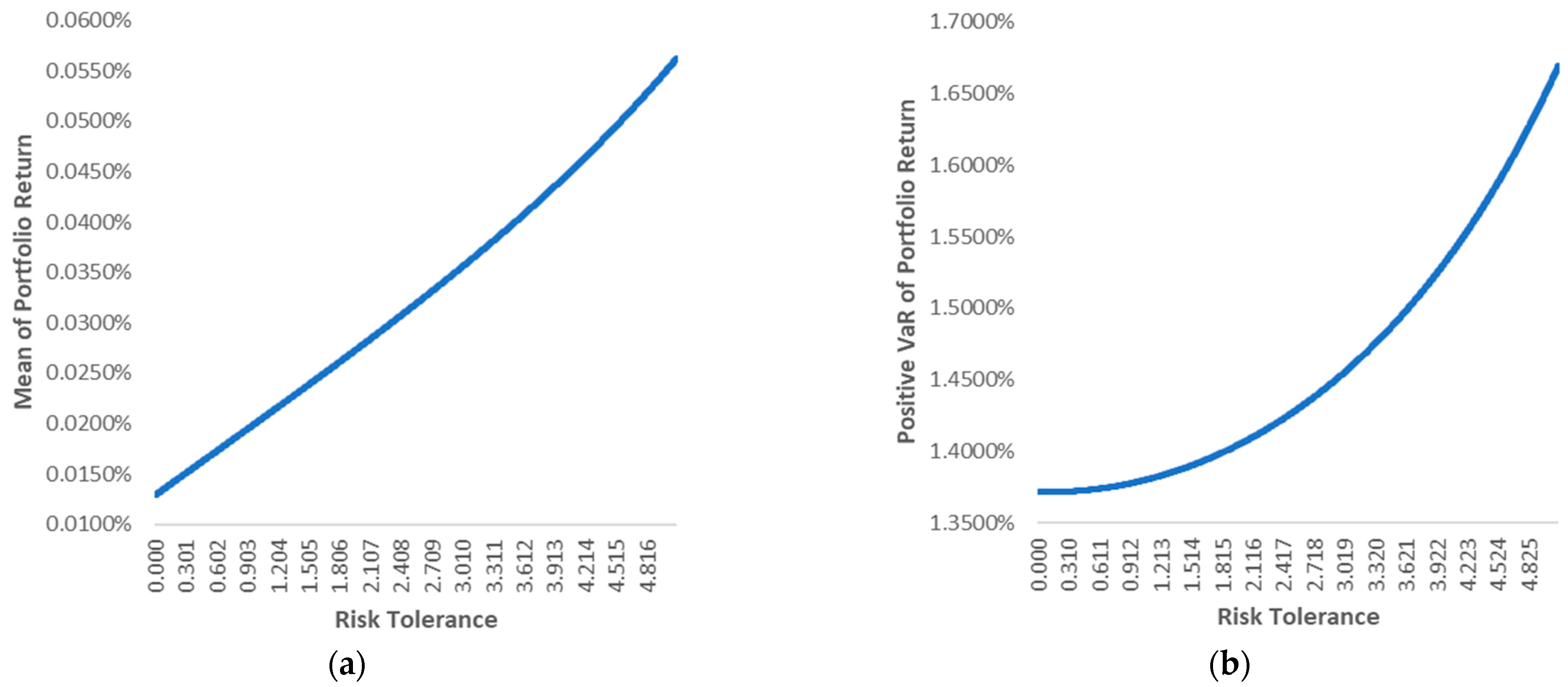
The designed mechanism is then applied to Indonesia’s 100 stock index data. Experimental data also present the sensitivity of the critical variables involved. The results of the sensitivity analysis in this section all seem logical. It indicates that the stock selection and capital weighting mechanisms can describe the actual situation. Finally, we also compared the mechanism of this research (MI) with another mechanism, traditional mean-VaR (MII). Mean portfolio return from MI is achieved or even exceeds it. In contrast, the mean of portfolio return from MII is not achieved and is even negative. These results indicate that clustering and analysis of stock price movements should be carried out in forming a stock portfolio.

As a suggestion for future mechanism development, the loss probability value in Equation (11) can be involved theoretically without being assumed to be a constant value in the actual number interval between zero and one. However, this will make determining the solution of the mean-VaR model more complex. This solution can be sought using the genetic algorithm method as a further suggestion. Then, the use of MACD can be combined with other indicators to estimate rising stock price trends more accurately. In addition, MACD also needs to be used for conditional conditions, such as when economic chaos occurs. In other words, the jumping effect on stock returns, which often occurs in stocks in large stock markets such as in the United States of America, can be considered. The jumping effect can be accommodated using the jumping process.

This research academically develops a portfolio design mechanism by clustering stocks and analyzing its price movement trends, enabling investors to practically diversify and choose stocks with increasing price trends, reducing losses, and increasing profit opportunities.

References

1. Boyle, P.; Garlappi, L.; Uppal, R.; Wang, T. Keynes Meets Markowitz: The Trade-Off Between Familiarity and Diversification. Manag. Sci. 2012, 58, 253–272. [Google Scholar] [CrossRef]
2. Kirby, C.; Ostdiek, B. It’s All in the Timing: Simple Active Portfolio Strategies That Outperform Naïve Diversification. J. Financ. Quant. Anal. 2012, 47, 437–467. [Google Scholar] [CrossRef]
3. Xiong, J.; Zhou, X.Y. Mean-Variance Portfolio Selection under Partial Information. SIAM J. Control Optim. 2007, 46, 156–175. [Google Scholar] [CrossRef]
4. Chan, K.; Hameed, A. Stock Price Synchronicity and Analyst Coverage in Emerging Markets. J. Financ. Econ. 2006, 80, 115–147. [Google Scholar] [CrossRef]
5. Chen, L.-H.; Huang, L. Portfolio Optimization of Equity Mutual Funds with Fuzzy Return Rates and Risks. Expert Syst. Appl. 2009, 36, 3720–3727. [Google Scholar] [CrossRef]
6. Sinha, P.; Chandwani, A.; Sinha, T. Algorithm of Construction of Optimum Portfolio of Stocks Using Genetic Algorithm. Int. J. Syst. Assur. Eng. Manag. 2015, 6, 447–465. [Google Scholar] [CrossRef]
7. Golosnoy, V.; Okhrin, Y. Flexible Shrinkage in Portfolio Selection. J. Econ. Dyn. Control 2009, 33, 317–328. [Google Scholar] [CrossRef]
8. Ren, F.; Lu, Y.-N.; Li, S.-P.; Jiang, X.-F.; Zhong, L.-X.; Qiu, T. Dynamic Portfolio Strategy Using Clustering Approach. PLoS ONE 2017, 12, e0169299. [Google Scholar] [CrossRef]
9. Fleischhacker, A.; Lettner, G.; Schwabeneder, D.; Auer, H. Portfolio Optimization of Energy Communities to Meet Reductions in Costs and Emissions. Energy 2019, 173, 1092–1105. [Google Scholar] [CrossRef]
10. Tola, V.; Lillo, F.; Gallegati, M.; Mantegna, R.N. Cluster Analysis for Portfolio Optimization. J. Econ. Dyn. Control 2008, 32, 235–258. [Google Scholar] [CrossRef]
11. Musmeci, N.; Aste, T.; Di Matteo, T. Relation between Financial Market Structure and the Real Economy: Comparison between Clustering Methods. PLoS ONE 2015, 10, e0116201. [Google Scholar] [CrossRef] [PubMed]
12. Hussain, W.; Merigó, J.; Raza, M.; Gao, H. A New QoS Prediction Model Using Hybrid IOWA-ANFIS with Fuzzy C-Means, Subtractive Clustering and Grid Partitioning. Inf. Sci. 2022, 584, 280–300. [Google Scholar] [CrossRef]
13. Chen, B.; Zhong, J.; Chen, Y. A Hybrid Approach for Portfolio Selection with Higher-Order Moments: Empirical Evidence from Shanghai Stock Exchange. Expert Syst. Appl. 2020, 145, 113104. [Google Scholar] [CrossRef]
14. Cheong, D.; Kim, Y.M.; Byun, H.W.; Oh, K.J.; Kim, T.Y. Using Genetic Algorithm to Support Clustering-Based Portfolio Optimization by Investor Information. Appl. Soft Comput. 2017, 61, 593–602. [Google Scholar] [CrossRef]
15. Khan, A.Z.; Mehlawat, M.K. Dynamic Portfolio Optimization Using Technical Analysis-based Clustering. Int. J. Intell. Syst. 2022, 37, 6978–7057. [Google Scholar] [CrossRef]
16. Vásquez Sáenz, J.; Quiroga, F.M.; Bariviera, A.F. Data vs. Information: Using Clustering Techniques to Enhance Stock Returns Forecasting. Int. Rev. Financ. Anal. 2023, 88, 102657. [Google Scholar] [CrossRef]
17. Navarro, M.M.; Young, M.N.; Prasetyo, Y.T.; Taylar, J.V. Stock Market Optimization amidst the COVID-19 Pandemic: Technical Analysis, K-Means Algorithm, and Mean-Variance Model (TAKMV) Approach. Heliyon 2023, 9, e17577. [Google Scholar] [CrossRef] [PubMed]
18. Aheer, A.K.; Pradhan, A.K.; Srivastava, R. Application of Feedforward Neural Network in Portfolio Optimization and Geometric Brownian Motion in Stock Price Prediction. In Proceedings of the 2023 4th International Conference on Electronics and Sustainable Communication Systems (ICESC), Coimbatore, India, 6–8 July 2023; IEEE: Piscataway, NJ, USA, 2023; pp. 1494–1503. [Google Scholar]
19. Hasbullah, E.S.; Halim, N.B.A.; Sukono; Putra, A.S.; Bon, A.T. Mean-Variance Portfolio Optimization on Islamic Stocks by Using Non Constant Mean and Volatility Models and Genetic Algorithm. Int. J. Eng. Technol. 2018, 7, 366. [Google Scholar] [CrossRef]
20. Du, X.; Tanaka-Ishii, K. Stock Portfolio Selection Balancing Variance and Tail Risk via Stock Vector Representation Acquired from Price Data and Texts. Knowl.-Based Syst. 2022, 249, 108917. [Google Scholar] [CrossRef]
21. Chang, R.-H.; Young, M.N.; Hildawa, M.I.; Santos, I.J.R.; Pan, C.-H. Portfolio Selection Problem Considering Behavioral Stocks. In Proceedings of the World Congress on Engineering (WCE) 2015, London, UK, 1–3 July 2015; Lecture Notes in Engineering and Computer Science. pp. 685–690. [Google Scholar]
22. Varga-Haszonits, I.; Kondor, I. Noise Sensitivity of Portfolio Selection in Constant Conditional Correlation GARCH Models. Phys. A Stat. Mech. Appl. 2007, 385, 307–318. [Google Scholar] [CrossRef]
23. Thuankhonrak, P.; Rattagan, E.; Phoomvuthisarn, S. Machine Trading by Time Series Models and Portfolio Optimization. In Proceedings of the 2019 4th International Conference on Information Technology (InCIT), Bangkok, Thailand, 24–25 October 2019; IEEE: Piscataway, NJ, USA; pp. 217–222. [Google Scholar]
24. Markowitz, H. Portfolio Selection. J. Financ. 1952, 7, 77–91. [Google Scholar] [CrossRef]
25. Sharpe, W.F. A Simplified Model for Portfolio Analysis. Manag. Sci. 1963, 9, 277–293. [Google Scholar] [CrossRef]
26. Sharpe, W.F. A Linear Programming Approximation for the General Portfolio Analysis Problem. J. Financ. Quant. Anal. 1971, 6, 1263. [Google Scholar] [CrossRef]
27. Young, M.R. A Minimax Portfolio Selection Rule with Linear Programming Solution. Manag. Sci. 1998, 44, 673–683. [Google Scholar] [CrossRef]
28. Björk, T.; Murgoci, A.; Zhou, X.Y. Mean-Variance Portfolio Optimization with State-Dependent Risk Aversion. Math. Financ. 2014, 24, 1–24. [Google Scholar] [CrossRef]
29. Abdurakhman, A. Asset Allocation in Indonesian Stocks Using Portfolio Robust. Math. Stat. 2022, 10, 1313–1319. [Google Scholar] [CrossRef]
30. Faramarzi, A.; Heidarinejad, M.; Stephens, B.; Mirjalili, S. Equilibrium Optimizer: A Novel Optimization Algorithm. Knowl.-Based Syst. 2020, 191, 105190. [Google Scholar] [CrossRef]
31. Zhou, X.Y.; Li, D. Continuous-Time Mean-Variance Portfolio Selection: A Stochastic LQ Framework. Appl. Math. Optim. 2000, 42, 19–33. [Google Scholar] [CrossRef]
32. Zhu, H.; Wang, Y.; Wang, K.; Chen, Y. Particle Swarm Optimization (PSO) for the Constrained Portfolio Optimization Problem. Expert Syst. Appl. 2011, 38, 10161–10169. [Google Scholar] [CrossRef]
33. Kalfin, S.; Carnia, E. Portfolio Optimization of the Mean-Absolute Deviation Model of Some Stocks Using the Singular Covariance Matrix. Int. J. Recent Technol. Eng. 2019, 8, 7818–7822. [Google Scholar] [CrossRef]
34. Ryoo, H.S. A Compact Mean-Variance-Skewness Model for Large-Scale Portfolio Optimization and Its Application to the NYSE Market. J. Oper. Res. Soc. 2007, 58, 505–515. [Google Scholar] [CrossRef]
35. Wang, J.; Gan, X. Neurodynamics-Driven Portfolio Optimization with Targeted Performance Criteria. Neural Netw. 2023, 157, 404–421. [Google Scholar] [CrossRef] [PubMed]
36. Mba, J.C.; Ababio, K.A.; Agyei, S.K. Markowitz Mean-Variance Portfolio Selection and Optimization under a Behavioral Spectacle: New Empirical Evidence. Int. J. Financ. Stud. 2022, 10, 28. [Google Scholar] [CrossRef]
37. Du, J. Mean–Variance Portfolio Optimization with Deep Learning Based-Forecasts for Cointegrated Stocks. Expert Syst. Appl. 2022, 201, 117005. [Google Scholar] [CrossRef]
38. Li, X.; Uysal, A.S.; Mulvey, J.M. Multi-Period Portfolio Optimization Using Model Predictive Control with Mean-Variance and Risk Parity Frameworks. Eur. J. Oper. Res. 2022, 299, 1158–1176. [Google Scholar] [CrossRef]
39. Ranković, V.; Drenovak, M.; Urosevic, B.; Jelic, R. Mean-Univariate GARCH VaR Portfolio Optimization: Actual Portfolio Approach. Comput. Oper. Res. 2016, 72, 83–92. [Google Scholar] [CrossRef]
40. Ashrafzadeh, M.; Taheri, H.M.; Gharehgozlou, M.; Hashemkhani Zolfani, S. Clustering-Based Return Prediction Model for Stock Pre-Selection in Portfolio Optimization Using PSO-CNN+MVF. J. King Saud Univ.-Comput. Inf. Sci. 2023, 35, 101737. [Google Scholar] [CrossRef]
41. Jain, A.K. Data Clustering: 50 Years beyond K-Means. Pattern Recognit. Lett. 2010, 31, 651–666. [Google Scholar] [CrossRef]
42. Chong, T.T.-L.; Ng, W.-K. Technical Analysis and the London Stock Exchange: Testing the MACD and RSI Rules Using the FT30. Appl. Econ. Lett. 2008, 15, 1111–1114. [Google Scholar] [CrossRef]
43. Hidayat, Y.; Purwandari, T.; Sukono; Prihanto, I.G.; Hidayana, R.A.; Ibrahim, R.A. Mean-Value-at-Risk Portfolio Optimization Based on Risk Tolerance Preferences and Asymmetric Volatility. Mathematics 2023, 11, 4761. [Google Scholar] [CrossRef]
44. Rosillo, R.; de la Fuente, D.; Brugos, J.A.L. Technical Analysis and the Spanish Stock Exchange: Testing the RSI, MACD, Momentum and Stochastic Rules Using Spanish Market Companies. Appl. Econ. 2013, 45, 1541–1550. [Google Scholar] [CrossRef]
45. Wang, J.; Kim, J. Predicting Stock Price Trend Using MACD Optimized by Historical Volatility. Math. Probl. Eng. 2018, 2018, 9280590. [Google Scholar] [CrossRef]
46. Purwandari, T.; Riaman; Hidayat, Y.; Sukono; Ibrahim, R.A.; Hidayana, R.A. Selecting and Weighting Mechanisms in Stock Portfolio Design Based on Clustering Algorithm and Price Movement Analysis. Mathematics 2023, 11, 4151. [Google Scholar] [CrossRef]
47. Madhulatha, T.S. An Overview on Clustering Methods. IOSR J. Eng. 2012, 2, 719–725. [Google Scholar] [CrossRef]
48. Kanungo, T.; Mount, D.M.; Netanyahu, N.S.; Piatko, C.D.; Silverman, R.; Wu, A.Y. An Efficient K-Means Clustering Algorithm: Analysis and Implementation. IEEE Trans. Pattern Anal. Mach. Intell. 2002, 24, 881–892. [Google Scholar] [CrossRef]
49. Hidayana, R.A.; Napitupulu, H.; Sukono, S. An Investment Decision-Making Model to Predict the Risk and Return in Stock Market: An Application of ARIMA-GJR-GARCH. Decis. Sci. Lett. 2022, 11, 235–246. [Google Scholar] [CrossRef]
50. Rankovic, V.; Drenovak, M.; Stojanovic, B.; Kalinic, Z.; Arsovski, Z. The Mean-Value at Risk Static Portfolio Optimization Using Genetic Algorithm. Comput. Sci. Inf. Syst. 2014, 11, 89–109. [Google Scholar] [CrossRef]
51. Ibrahim, R.A.; Sukono; Napitupulu, H.; Ibrahim, R.I. How to Price Catastrophe Bonds for Sustainable Earthquake Funding? A Systematic Review of the Pricing Framework. Sustainability 2023, 15, 7705. [Google Scholar] [CrossRef]
52. Bowling, S.R.; Khasawneh, M.T.; Kaewkuekool, S.; Cho, B.R. A Logistic Approximation to the Cumulative Normal Distribution. J. Ind. Eng. Manag. 2009, 2, 114–127. [Google Scholar] [CrossRef]
53. Sukono; Ibrahim, R.A.; Saputra, M.P.A.; Hidayat, Y.; Juahir, H.; Prihanto, I.G.; Halim, N.B.A. Modeling Multiple-Event Catastrophe Bond Prices Involving the Trigger Event Correlation, Interest, and Inflation Rates. Mathematics 2022, 10, 4685. [Google Scholar] [CrossRef]
54. Sinaga, J.; Wu, T.; Chen, Y. Impact of Government Interventions on the Stock Market during COVID-19: A Case Study in Indonesia. SN Bus. Econ. 2022, 2, 136. [Google Scholar] [CrossRef] [PubMed]
55. Rousseeuw, P.J. Silhouettes: A Graphical Aid to the Interpretation and Validation of Cluster Analysis. J. Comput. Appl. Math. 1987, 20, 53–65. [Google Scholar] [CrossRef]
56. Tibshirani, R.; Walther, G.; Hastie, T. Estimating the Number of Clusters in a Data Set Via the Gap Statistic. J. R. Stat. Soc. Ser. B Stat. Methodol. 2001, 63, 411–423. [Google Scholar] [CrossRef]
57. Lo, A.W. The Statistics of Sharpe Ratios. Financ. Anal. J. 2002, 58, 36–52. [Google Scholar] [CrossRef]
Figure 2. K-means clustering method algorithm.
Mathematics 12 00174 g002
Figure 3. Stocks with a positive mean of return on the Kompas 100 Index in Indonesia.
Mathematics 12 00174 g003
Figure 4. Average silhouette width value of each cluster.
Mathematics 12 00174 g004
Figure 5. Relationship between mean and VaR of portfolio return.
Mathematics 12 00174 g005
Figure 6. Sensitivity of buy transaction costs (a), sell transaction costs (b), income tax (c), portfolio loss probability (d), and z α (e) to the mean of portfolio return.
Mathematics 12 00174 g006aMathematics 12 00174 g006b
Figure 7. Sensitivity of selling transaction costs (a), income tax (b), portfolio loss opportunities (c), and z α (d) to the standard deviation of portfolio returns.
Mathematics 12 00174 g007
Figure 8. Sensitivity of risk tolerance to mean (a) and VaR (b) of portfolio returns.
Mathematics 12 00174 g008