Compound Optimum Designs for Clinical Trials in Personalized Medicine

Abstract

We consider optimal designs for clinical trials when response variance depends on treatment and covariates are included in the response model. These designs are generalizations of Neyman allocation, and commonly employed in personalized medicine where external covariates linearly affect the response. Very often, these designs aim at maximizing the amount of information gathered but fail to assure ethical requirements. We analyze compound optimal designs that maximize a criterion weighting the amount of information and the reward of allocating the patients to the most effective/least risky treatment. We develop a general representation for static (a priori) allocation and propose a semidefinite programming (SDP) formulation to support their numerical computation. This setup is extended assuming the variance and the parameters of the response of all treatments are unknown and an adaptive sequential optimal design scheme is implemented and used for demonstration. Purely information theoretic designs for the same allocation have been addressed elsewhere, and we use them to support the techniques applied to compound designs.

1. Introduction

This paper investigates methods for optimizing experimental designs in clinical trials, focusing on maximizing the information needed to predict responses to various treatments while considering ethical constraints relevant to personalized medicine. We extend existing approaches by addressing the challenge of patient allocation to treatments, aiming to balance statistical efficiency with the ethical imperative of minimizing the risk of administering suboptimal treatments to new patients. Our interest in personalized medicine leads to the modeling of patient–treatment interactions. Consequently, there is generally no single best treatment; the optimal choice depends on the patient’s covariates. Common patient covariates, also known as prognostic factors, include age, sex, prior illnesses, and baseline status on various indicators such as depression and susceptibility to certain conditions. These covariates may be represented by continuous metrics or discrete scales. Despite the differences in their nature, the challenge of optimally allocating patients remains a general problem, regardless of the type of covariates involved.

The main challenges in optimally allocating patients to effective treatments in clinical trials are (i) patient heterogeneity: variability among patients makes it difficult to predict individual responses to different treatments; (ii) ethical considerations: ensuring equitable access to potentially effective treatments for all participants while maintaining scientific rigor; (iii) bias and randomization: proper randomization is essential to avoid skewed results and the effects of uncontrolled factors, so as to ensure accurate assessments of treatment effectiveness; (iv) treatment effectiveness: identifying the most effective treatment for various patient subgroups can be challenging; (v) sample size and power: determining appropriate sample sizes is crucial for detecting meaningful differences between treatments; and (vi) dynamic changes in patient status: variations in patients’ conditions over time can affect treatment effectiveness and influence trial conclusions [1]. In this study, we focus on points (ii) through (vi) and examine methods to address these challenges.

The problem of prescribing optimal designs in clinical trials is formalized as the maximization of a compound optimal design criterion that balances the information gained from the trial with the goal of maximizing patient outcomes by allocating them to the most effective treatments. While the first component of the objective function, related to statistical information, was discussed in Duarte and Atkinson [2], the second component addresses ethical concerns.

Typically, clinical trials are designed to either (i) maximize the information that enhances statistical inference about the response models; or (ii) satisfy ethical requirements by ensuring each patient is allocated to the most effective treatment as that becomes evident. These objectives often conflict with each other, leading to the formulation of an optimal allocation problem that may (i) maximize the information gained while imposing an upper limit on regret arising from allocation of patients to treatments which are not the best for them; or (ii) minimize regret while constraining the amount of information obtained, typically measured by a suitable convex function of the Fisher information matrix (FIM). When both objectives are convex (or concave), they can be combined using a linear combination with a Lagrange coefficient. This approach facilitates a balanced compromise between the incremental gain in information and the ethical considerations associated with treatment allocation [3,4].

In this paper, we consider the standard model commonly used in clinical trials, as described by Rosenberger and Lachin [5]. This model for the expected response to a given treatment includes a linear component to account for the effects of prognostic factors, or covariates, along with an additive constant representing the treatment effect [6]. The coefficients that link the covariates to the response for each treatment are either known a priori or can be sequentially estimated by fitting previous responses using least-squares methods. The response is assumed to follow a normal distribution, with each treatment associated with a distinct level of observational noise variance, which may be known beforehand or estimated from trial data. Such dependence of response variance on treatment is an extension of the standard model of Rosenberger and Lachin [5]. A second extension of the standard model is the existence of patient–treatment interactions.

Hu et al. [7] proposed a general family of covariate-adaptive, response-adaptive designs and derived the asymptotic properties of optimal allocation schemes. Additionally, Atkinson [8] presented optimal experimental designs for regression models—those with covariates—specifically when there are two treatments with differing variances. In this setup, a single normal response model is applied to all subjects. An up-to-date review of this topic can be found in Sverdlov et al. [9].

The use of compound criteria to identify sequential optimal designs is an area of active research, with the primary goal of reconciling the two key objectives of maximizing information and addressing ethical considerations. To incorporate ethical concerns into the optimal design criterion, a method based on randomly reinforced urn designs was applied, as detailed in May and Flournoy [10]. In a similar vein, Antognini and Giovagnoli [11] explored problems without covariates, integrating standardized information and ethical measures into the optimality criterion. Their approach dynamically adjusts the weight on the two components based on the observed outcomes. Sverdlov et al. [12] examined responses related to time-to-event data, also without covariates. Furthermore, Metelkina and Pronzato [13] proposed a covariate-adaptive sequential allocation strategy that converges to the optimum, demonstrating the equivalence of this approach to penalized designs.

The numerical computation of compound designs that incorporate ethical considerations poses significant challenges, often hindering their practical application. In many cases, the computational complexity of these designs makes their implementation in real-world settings challenging. Consequently, decision makers (such as physicians and other agents) often opt for simpler methods that offer greater interpretability and can be more easily integrated into suitable information systems [14]. This paper addresses this issue by introducing a semidefinite programming formulation to derive asymptotic designs, along with a sequential allocation algorithm suited for real-world scenarios where prior knowledge is limited and the model parameters and response variance are extracted from individuals’ responses.

Our approach automates the computation of standardized compound designs by using the D-optimality criterion to measure information and quantifying rewards based on the expected response. The framework assumes known treatment variances and determines the optimal (continuous) designs for patient allocation across treatments. The information component in our compound designs is grounded in the Neyman allocation method, incorporating covariates as previously explored in Duarte and Atkinson [2]. The ethics-based component is represented by the reward of the response, which is determined by the expectation calculated over a finitely large patient sample. When employing sequential designs, this expectation can also be iteratively approximated using a finite sample with known response values.

Further, we also address the more common scenario where treatment response variances and coefficients are initially unknown. In this case, we propose a sequential optimal design framework that updates the model after each patient response is obtained, subsequently allocating the next patient to the treatment that maximizes the compound objective.

This paper introduces three key innovations: (i) the development of a framework that enables the computation of compound designs incorporating standardized information measures and regret components; (ii) the formulation of semidefinite programming (SDP) methods to generalize the numerical computation of these designs; and (iii) the creation of an adaptive optimal allocation scheme that updates both the models for the responses and response variances in real time.

The paper is organized as follows. Section 2 provides the background and introduces the notation used for the problem formulation. Section 3 outlines the problem of optimal allocation using the compound-standardized information–regret (I-R) criterion. Section 4 presents the semidefinite programming (SDP) formulations designed to systematically address the problem; the construction of normalization values for computing normalized regret is detailed in Appendix A. Section 5 describes the algorithm for determining optimal sequential allocation designs, which is illustrated with an example. In Section 6, we apply the proposed methodologies to a real-world case, specifically focusing on the optimal allocation of Parkinson’s disease patients to two alternative care treatments. Finally, in Section 7, we conclude with a brief discussion of our results.

2. Notation and Background

This section establishes the nomenclature and fundamental background used in the subsequent sections.

In our notation, boldface lowercase letters represent vectors, boldface capital letters represent continuous domains, blackboard bold capital letters denote discrete domains, and capital letters are used for matrices. Finite sets with $\iota$ elements are compactly represented by $⟦\iota ⟧\equiv \{1,\dots ,\iota \}$. The transpose operation of a matrix or vector is denoted by ${“}^{\mathsf{T}}$”. The determinant of a matrix is represented by $det(•)$, and the trace is denoted by $tr(•)$. The nomenclature used throughout the paper is provided at the end.

Let $k\in ⟦K⟧$ denote the covariates in the linear response model, $i\in ⟦I⟧$ represent the treatments, and $j\in ⟦J⟧$ indicate the levels each factor can have in the experiment. Here, K, I, and J denote the number of covariates, treatments, and factor levels in the response model, respectively.

When $i\in \{1,2\}$ (indicating two treatments) and there are k covariates, the response model is given by

$$\begin{array}{cc}\hfill {\eta }_1(\mathbf{x},\mathit{\theta })& ={\alpha }_1+{\beta }_{1,1}{x}_1+{\beta }_{1,2}{x}_2+\cdots +{\beta }_{1,K}{x}_K,\mathrm{var}\left({\eta }_1\right)={\sigma }_1^2,\hfill \end{array}$$

(1a)

$$\begin{array}{cc}\hfill {\eta }_2(\mathbf{x},\mathit{\theta })& ={\alpha }_2+{\beta }_{2,1}{x}_1+{\beta }_{2,2}{x}_2+\cdots +{\beta }_{2,K}{x}_K,\mathrm{var}\left({\eta }_2\right)={\sigma }_2^2,\hfill \end{array}$$

(1b)

where $\mathbf{x}=(x_1,x_2,\dots ,x_K)\in \mathbf{X}\subset {\mathbb{R}}^K$ is the vector of covariates, $\mathbf{X}$ denotes the design space which contains all possible values of $\mathbf{x}$, $\mathit{\theta }$ represents the set of parameters to be estimated (including all $\alpha$’s and $\beta$’s), and $\mathrm{\Theta }\subset {\mathbb{R}}^{n_{\theta }}$ is the domain of these parameters, with $n_{\theta }$ being the total number of parameters across all treatment models. The models ${\eta }_i(\mathbf{x},\mathit{\theta })$, for $i\in ⟦2⟧$, represent the expected responses, each characterized by an error term with variance $\mathrm{var}\left({\eta }_i\right)$. The pth realization of $\mathbf{x}$ characterizing the pth patient is represented as ${\mathbf{x}}_p$.

The allocation is optimized to maximize the information extracted from patients’ responses while considering the predictions from the model. Our goal is to determine the allocation of individuals to treatment 1 for estimating the parameters ${({\alpha }_1,{\beta }_{1,1},\dots ,{\beta }_{1,K})}^{\mathsf{T}}$, and to treatment 2 for estimating the parameters of the second treatment model. In approximate optimal designs, w represents the fraction of individuals allocated to treatment 1, while $1-w$ denotes the fraction allocated to treatment 2. This yields the design matrix

$$\xi =\left(\begin{array}{ccc}w& & 1-w\\ 1& & 2\end{array}\right).$$

Here, the upper row of $\xi$ indicates the fraction allocated to each treatment, while the lower row denotes the treatment number itself. In cases where the number of individuals is small and an exact design is required, rounding procedures can be used to determine the allocation, as described in Pukelsheim and Rieder [15].

Let $\tau ={\sigma }_2^2/{\sigma }_1^2$, and without loss of generality, let ${\sigma }_1^2=1$. Consequently, the Fisher information matrix (FIM) for the experimental design $\xi$ is a $2(K+1)\times 2(K+1)$ diagonal matrix given by Atkinson [8]:

$$\begin{array}{c}\hfill M\left(\xi \right)=\left(\begin{array}{ccccc}w& 0& \cdots & 0& 0\\ 0& {\displaystyle \frac{1-w}{\tau }}& \cdots & 0& 0\\ ⋮& ⋮& \ddots & ⋮& ⋮\\ 0& 0& \cdots & w& 0\\ 0& 0& \cdots & 0& {\displaystyle \frac{1-w}{\tau }}\end{array}\right).\end{array}$$

(2)

3. Standardized Compound Designs

In this section, we formulate standardized compound designs that balance information measurement criteria with regret. The response models for all treatments are continuous and exhibit linear dependence on K covariates. Moreover, the variances of the treatment responses are known a priori. Our goal is to establish a general conceptual framework for determining continuous optimal information–regret (I-R) designs, characterized by the fraction of patients allocated to each treatment.

We focus on the computation of I-R designs, which aim to reconcile the objectives of allocating individuals to the most promising treatments while optimizing parameter estimation efficiency across different response groups; see Hu et al. [7], Antognini and Giovagnoli [11], Metelkina and Pronzato [13]. In most applications, responses are either binary or follow a standard linear model. For both types, it is rational to evaluate allocation procedures based on the proportion of patients receiving the most effective treatment. However, in the presence of patient–treatment interactions, there is generally no single best treatment; the optimal choice depends on the patient’s covariates. If the responses are significantly different, the choice of treatment is crucial. Conversely, if the responses are similar, the advantage of one treatment over another is minimal. Thus, we use the expected response value based on previous allocations as our indicator for correct allocation. This approach represents an innovation compared to earlier methods.

This problem is particularly relevant as it mirrors the sequential allocation of individuals in clinical trials. It exploits prior information—characterized by both continuous and discrete covariates known a priori—to refine allocation strategies in later stages. Practically, optimization strategies offer significant advantages over pure randomization techniques, as discussed in Bertsimas et al. [16], Kallus [17].

In this context, we integrate standardized D-optimality, which quantifies the information content, with standardized regret, which measures the expected loss associated with not selecting the optimal treatment—the one corresponding to the highest response.

We first consider the information criterion. Assume the covariates $x_k$ for $k\in ⟦K⟧$ are discrete, taking values in $\{-1,+1\}$. Consequently, the design space is defined as $\mathbf{X}\equiv {\{-1,+1\}}^K$. Let $\mathit{\theta }$ denote the set of parameters to be estimated, including the vectors $\mathit{\alpha }$ and $\mathit{\beta }$ in Equation (1). In this simplified configuration, we consider categorical covariates with two levels: $-1$ (lower) and $+1$ (upper). According to the bound on the determinant of a Hadamard matrix [18,19], extreme observations provide the most information for the D-optimality criterion in first-order models.

We emphasize that using these limited support points for the designs helps reduce the computational burden when demonstrating the properties of our designs in a non-sequential context and provides valuable asymptotic allocations. In the application to constructing sequential clinical trials discussed in Section 5, covariate values are sampled from continuous distributions.

The criterion used for information-theoretical analysis in this work is D-optimality. This approach aims to maximize the determinant of the matrix $M\left(\xi \right)$, or equivalently, the $1/\left[2\right(K+1\left)\right]$ power of the determinant, which represents the geometric mean of the diagonal elements of matrix B, as described in Duarte and Atkinson [2] (Equation 3.d).

To address our objective of integrating criteria that measure different aspects—specifically, the information content in the allocation and the regret associated with individual treatment assignments—we use standardized criteria, as detailed by Dette [20]. Hence, the information criterion we seek to maximize is given by

$$\begin{array}{cc}\hfill \mathrm{\Psi }(\xi ,\mathit{\theta })& ={\left({\displaystyle \frac{det\left[M\right(\xi ,\mathit{\theta }\left)\right]}{det\left[M({\xi }^{*},\mathit{\theta })\right]}}\right)}^{1/n_{\theta }}\hfill \end{array}$$

(3a)

$$\begin{array}{cc}\hfill M(\xi ,\mathit{\theta })& =\sum _{i=1}^I{w}_i\mathcal{M}({\eta }_i,\mathit{\theta })\hfill \end{array}$$

(3b)

$$\begin{array}{cc}\hfill \mathcal{M}({\eta }_i,\mathit{\theta })& ={\left({\displaystyle \frac{\partial {\eta }_i(\mathbf{x},\mathit{\theta })}{\partial \mathit{\theta }}}\right)}^{\mathsf{T}}\left({\displaystyle \frac{\partial {\eta }_i(\mathbf{x},\mathit{\theta })}{\partial \mathit{\theta }}}\right),\hfill \end{array}$$

(3c)

where $\mathcal{M}({\eta }_i,\mathit{\theta })$ represents the Fisher information matrix (FIM) for treatment i, and ${\xi }^{*}$ denotes the optimal allocation when D-optimality is the sole criterion. For simplicity, we assume the models ${\eta }_i(•)$ are linear in parameters, which makes the matrices $\mathcal{M}({\eta }_i,\mathit{\theta })$ independent of $\mathit{\theta }$. The explicit inclusion of $\mathit{\theta }$ in the definition of $\mathrm{\Psi }(\xi ,\mathit{\theta })$ serves two main purposes: (i) it clarifies the dependency on the number of parameters; and (ii) it aligns the functional with the regret representation, which does depend on $\mathit{\theta }$.

We now introduce the regret criterion. The objective is to assign an individual, denoted as individual $m+1$, who is characterized by covariate values ${\mathbf{x}}_{m+1}$, to the treatment that maximizes the expected response. For simplicity, we assume that higher response values are preferred, although the opposite preference could also be applied.

To align this criterion with the information criterion, it is necessary to normalize the responses to fall within the range $[0,1]$. To achieve this normalization, we need to evaluate all I treatments and, for each treatment, consider all possible covariate values in ${\mathrm{\Omega }}_m\equiv {\left\{\mathbf{x}\right\}}_1^m$. Here, ${\mathrm{\Omega }}_m$ includes the m previous vectors of covariates that have already been allocated. Assuming perfect knowledge of the parameters $\mathit{\theta }$ for all models, let

$$y_{{\mathrm{\Omega }}_m}^{max}=\underset{i\in ⟦I⟧}{max}\underset{\mathbf{x}\in {\mathrm{\Omega }}_m}{max}{\eta }_i(\mathbf{x},\mathit{\theta })$$

denote the maximum response value achieved by the treatment that yields the highest response. Specifically, $y_{{\mathrm{\Omega }}_m}^{max}$ represents the highest value of the response over all models $i\in ⟦I⟧$ and covariate values $\mathbf{x}\in {\mathrm{\Omega }}_m$, obtained using model (1).

Conversely, the minimum response is denoted by $y_{{\mathrm{\Omega }}_m}^{min}$, which satisfies

$$y_{{\mathrm{\Omega }}_m}^{min}=\underset{i\in ⟦I⟧}{min}\underset{\mathbf{x}\in {\mathrm{\Omega }}_m}{min}{\eta }_i(\mathbf{x},\mathit{\theta }).$$

Let

$$∆=y_{{\mathrm{\Omega }}_m}^{max}-y_{{\mathrm{\Omega }}_m}^{min}$$

(4)

denote the difference in response expectations between the “optimal” and “least favorable” treatments for $\mathbf{x}\in {\mathrm{\Omega }}_m$. Each of these values can be computed using the mixed-integer linear programming (MILP) procedure detailed in Appendix A. The parameter $∆$ ensures compatibility between the standardized regret and the standardized information criteria. To complete the scaling, we also need to determine the minimum response achieved (i.e., the baseline), denoted as

$${\delta }_{min}=y_{{\mathrm{\Omega }}_m}^{min}.$$

These problems determine the maximum (or minimum) response of a set of discrete points, considering the full set of response models. This approach is used to systematically find the extrema of possibly nonlinear or even discontinuous response models. We rely on a branch-and-cut large-scale solver [21], which ensures solvability even for larger numbers of discrete points and response models.

We now turn to the design of experiments. In the clinical trials motivating our work, the choice of covariate vector $\mathbf{x}$ is not under our control. Each patient p arrives with a predetermined covariate vector. The central design question is determining the most suitable treatment for each patient.

The optimal treatment allocation for the $p\mathrm{th}$ individual is given by the treatment $i_p^{max}$, which is defined as

$$i_p^{max}=arg\underset{i\in ⟦I⟧}{max}{\eta }_i({\mathbf{x}}_p,\mathit{\theta }),$$

where ${\eta }_i({\mathbf{x}}_p,\mathit{\theta })$ represents the response of treatment i given the covariate vector ${\mathbf{x}}_p$ and the parameter vector $\mathit{\theta }$.

In this context, regret measures the cost associated with not selecting the most effective treatment, as described by Rosenberger and Sverdlov [22]. When comparing different allocation strategies for I treatments across m individuals with known covariate information, regret is quantified as the average difference between the expected outcomes of the optimal allocation policy and those of an alternative policy.

Specifically, the non-standardized average regret, denoted as ${\mathrm{\Gamma }}^{\mathrm{ns}}$, is defined as

$${\mathrm{\Gamma }}_m^{\mathrm{ns}}(\xi ,\mathit{\theta })={\displaystyle \frac{1}{m}}\sum _{j=1}^m\left[y_{{\mathrm{\Omega }}_m}^{max}-{\eta }_{\ell \left(j\right)}({\mathbf{x}}_j,\mathit{\theta })\right],$$

(5)

where $y_{{\mathrm{\Omega }}_m}^{max}$ is the maximum expected response achievable across all treatments given the covariate information available, and ${\eta }_{\ell \left(j\right)}({\mathbf{x}}_j,\mathit{\theta })$ is the response of the treatment actually assigned to the $j\mathrm{th}$ individual. Here, ℓ denotes a vector, where $\ell \left(j\right)$ specifies the treatment assigned to the $j\mathrm{th}$ individual.

The scale factor used to normalize the average regret to the unit interval, $∆$, remains constant for optimal designs when the model coefficients of treatments are known. However, it must be re-estimated in sequential allocation schemes as new data become available. Given that

$$y_{{\mathrm{\Omega }}_m}^{max}=∆+{\delta }_{min},$$

the standardized average regret, referred to as “regret” (without superscript) in the following sections, is given by

$${\mathrm{\Gamma }}_m(\xi ,\mathit{\theta })={\displaystyle \frac{{\mathrm{\Gamma }}_m^{\mathrm{ns}}(\xi ,\mathit{\theta })+{\delta }_{min}}{∆}}.$$

Alternatively, ${\mathrm{\Gamma }}_m(\xi ,\mathit{\theta })$ can be expressed as

$${\mathrm{\Gamma }}_m(\xi ,\mathit{\theta })=1-{\displaystyle \frac{1}{m}}\sum _{j=1}^m{\displaystyle \frac{{\eta }_{\ell \left(j\right)}({\mathbf{x}}_j,\mathit{\theta })-{\delta }_{min}}{∆}},$$

(6)

where ${\eta }_{\ell \left(j\right)}({\mathbf{x}}_j,\mathit{\theta })$ represents the response of the treatment assigned to the $j\mathrm{th}$ individual.

Minimizing regret in the allocation process corresponds to selecting the treatment that maximizes the following objective function (up to constant terms):

$$\underset{\mathbf{w}}{max}\left[-{\mathrm{\Gamma }}_m(\xi ,\mathit{\theta })\right]\equiv \underset{i\in ⟦I⟧}{max}{\displaystyle \frac{1}{m}}\sum _{j=1}^m{\displaystyle \frac{{\eta }_{\ell \left(j\right)=i}({\mathbf{x}}_j,\mathit{\theta })-{\delta }_{min}}{∆}},$$

where $\mathbf{w}\in {\mathbb{R}}^I$ denotes the vector of proportions of patients allocated to each treatment, subject to the constraint ${\sum }_{i=1}^I{w}_i=1$.

Let $m_i$ (with $m_i<m$) denote the number of subjects previously assigned to treatment i. Consequently, we have

$$\begin{array}{cc}\hfill {\displaystyle \frac{1}{m}}\sum _{i=1}^I\sum _{j=1}^m{\displaystyle \frac{{\eta }_{\ell \left(j\right)=i}({\mathbf{x}}_j,\mathit{\theta })-{\delta }_{min}}{∆}}& =\sum _{i=1}^I{w}_i{\mathbb{E}}_m\left({\displaystyle \frac{{\eta }_i(\mathbf{x},\mathit{\theta })-{\delta }_{min}}{∆}}\right),\hfill \end{array}$$

(7)

where ${\mathbb{E}}_m\left({\displaystyle \frac{{\eta }_i(\mathbf{x},\mathit{\theta })-{\delta }_{min}}{∆}}\right)$ represents the expectation of the standardized loss for the $m_i$ individuals previously allocated to treatment i. For a detailed derivation of Equation (7), refer to Appendix B.

The I-R-optimality criterion is formulated by integrating the information-theoretic criterion from Equation (3) with the regret criterion from Equation (7). The I-R-optimal design seeks to address the following optimization problem:

$$\underset{\mathbf{w}\in {[0,1]}^I}{max}(1-\gamma )\mathrm{\Psi }(\xi ,\mathit{\theta })-\gamma {\mathrm{\Gamma }}_m(\xi ,\mathit{\theta })$$

which is equivalently expressed as

$$\underset{\mathbf{w}\in {[0,1]}^I}{max}(1-\gamma ){\left({\displaystyle \frac{det\left[M\right(\xi ,\mathit{\theta }\left)\right]}{det\left[M({\xi }^{*},\mathit{\theta })\right]}}\right)}^{1/n_{\mathit{\theta }}}+\gamma \sum _{i=1}^n{w}_i{\mathbb{E}}_m\left({\displaystyle \frac{{\eta }_i(\mathbf{x},\mathit{\theta })-{\delta }_{min}}{∆}}\right),$$

(8a)

$$\mathrm{s}.\mathrm{t}.\sum _{i=1}^I{w}_i=1\hspace{1em}\hspace{1em}\hspace{1em}\hspace{1em}\hspace{1em}\hspace{1em}\hspace{1em}\hspace{1em}\hspace{1em}\hspace{1em}\hspace{1em}\hspace{1em}\hspace{1em}\hspace{1em}\hspace{1em}\hspace{1em}\hspace{1em}\hspace{1em}\hspace{1em}\hspace{1em}\hspace{1em}\hspace{1em}$$

(8b)

where $\gamma \in [0,1]$ represents the relative weight assigned to the regret criterion, which is determined in advance. In practice, the decision maker selects this parameter to reflect the relative importance of ethical considerations versus inferential accuracy when developing response models for both groups. For instance, if $\gamma$ is set to 0.95, it suggests that ethical concerns are given 19 times more significance than the information criterion. This high value of $\gamma$ is typically used in scenarios where patients are well-informed, and the priority is to minimize regret by allocating them to the treatment with the least potential regret.

Problem (8) is formulated similarly to (Metelkina and Pronzato [13], Equation 2.9) and can also be represented as a semidefinite program. However, it is important to note that the multiplicative compound criterion proposed by Hu et al. [7] cannot be expressed in semidefinite form due to the lack of semidefinite representability of the functions involved. Additionally, when $\gamma =0$, the I-R-optimality criterion simplifies to D-optimality, as discussed in (Duarte and Atkinson [2], §4). On the other hand, when $\gamma =1$, the criterion aligns with concepts from multi-armed bandit theory, such as those explored by Villar et al. [23].

4. Optimal I-R Designs via SDP

We now present a formulation to address problem (8) using semidefinite programming. Solving this problem via SDP involves several key steps: (i) determining the value of $det\left[M({\xi }^{*},\mathit{\theta })\right]$ in Equation (3a), which can be precomputed using the procedure outlined in (Duarte and Atkinson [2], A1.a–A1.e). This corresponds to calculating the determinant for the optimal design when the objective is the D-optimality criterion. (ii) Estimating the average response of each treatment, a process that relies on the parameter vector $\mathit{\theta }$ derived from previous allocations and is inherently subject to noise. (iii) Computing the quantities $y_{{\mathrm{\Omega }}_m}^{min}$, $y_{{\mathrm{\Omega }}_m}^{max}$, $∆$, and ${\delta }_{min}$, as obtained from Equations (4), (A1) and (A2). (iv) Incorporating the weight $\gamma$, as specified by the user.

In practical terms, this design can be interpreted as an approximate, infinite-size local design intended to estimate a specific parameter vector $\mathit{\theta }$. The primary goal of this formulation is to establish an asymptotic framework for resolving local designs within sequential procedures, as outlined by Pocock [24]. The formulation is presented below.

$$\begin{array}{cc}\hfill \underset{\xi ,B,t}{max}& (1-\gamma ){\displaystyle \frac{t}{{\{det\left[M({\xi }^{*},\mathit{\theta })\right]\}}^{1/\left[2\right(K+1\left)\right]}}}+\gamma \sum _{i=1}^I{w}_i{\mathbb{E}}_m\left({\displaystyle \frac{{\eta }_i(\mathbf{x},\mathit{\theta })-{\delta }_{min}}{∆}}\right)\hfill \end{array}$$

(9a)

$$\begin{array}{cc}\hfill \mathrm{s}.\mathrm{t}.& \left(\begin{array}{cc}M(\xi ,\mathit{\theta })& B^{\mathsf{T}}\\ B& diag\left(B\right)\end{array}\right)⪰0_{4(K+1)}\hfill \end{array}$$

(9b)

$$\begin{array}{cc}\hfill & t\le \prod _{j=1}^{2(K+1)}{B}_{j,j}^{1/\left[2\right(K+1\left)\right]}\hfill \end{array}$$

(9c)

$$\begin{array}{cc}\hfill & \sum _{i=1}^I{w}_i=1\hfill \end{array}$$

(9d)

$$\begin{array}{cc}\hfill & 0\le w_i\le 1,i\in ⟦I⟧.\hfill \end{array}$$

(9e)

Here, B is a lower triangular matrix of size $2(K+1)\times 2(K+1)$, $B_{j,j},j\in ⟦2(K+1)⟧$ the diagonal elements of B, and t the hypograph of the determinant function.

To illustrate the application of Problem (9), consider a scenario similar to the one presented in Section 4 of Duarte and Atkinson [2]. In this setup, there are two treatments and two covariates (denoted as $x_1$ and $x_2$), each with two levels. The design space is defined as $\mathbf{X}\equiv {\{-1,+1\}}^2$. The local parameter values $\mathit{\theta }$ for treatment 1 are $({\alpha }_1,{\beta }_{1,1},{\beta }_{1,2})=(0.5,0.2,0.4)$, and for treatment 2 they are $({\alpha }_2,{\beta }_{2,1},{\beta }_{2,2})=(1.0,0.8,1.0)$. By solving programs (A1) and (A2), we obtain the following values: $y_{{\mathrm{\Omega }}_m}^{min}={\delta }_{min}=-0.8$, $y_{{\mathrm{\Omega }}_m}^{max}=2.8$, and $∆=3.6$. The expected values for each model are ${\mathbb{E}}_m\left[{\eta }_1(\mathbf{x},\mathit{\theta })\right]=0.5$ and ${\mathbb{E}}_m\left[{\eta }_2(\mathbf{x},\mathit{\theta })\right]=1.0$, respectively. This setup demonstrates that the second treatment has a significantly higher expected value, making it the preferable choice to minimize regret. However, it is crucial to recognize that decision making is also influenced by the uncertainty in the responses, as quantified by $\tau$, which in turn impacts the information-based criterion.

We systematically vary the parameter $\tau$ to conduct a comparative analysis between I-R-optimal designs and purely information-theoretical designs, as presented in Duarte and Atkinson [2]. For each value of $\tau$, we use the optimal $det\left[M({\xi }^{*},\mathit{\theta })\right]$ values from Table 1 in Duarte and Atkinson [2], which were derived for the case $K=2$. Additionally, we explore different values of $\gamma$ in the set $\{0.90,0.95\}$ to assess the impact of the weighting parameter, where a higher $\gamma$ emphasizes the importance of regret in the allocation process.

The performance of these designs depends on the values of $\mathbf{x}$. In our calculations, we assume an equal occurrence of each $\mathbf{x}$ value, resulting in balanced $2^K$ experiments for each treatment. The corresponding results are presented in

Table 1. I-R-optimal designs for model (1) (including two treatments, two covariates and $x_k\in \{-1,+1\},k\in ⟦K⟧$, and $w_2=1-w_1$).

${\mathit{\sigma }}_1^2$	${\mathit{\sigma }}_2^2$	I-R-Opt. Design †		I-R-Opt. Design ‡
		${\mathit{w}}_{\mathbf{1}}$	Opt	${\mathit{w}}_{\mathbf{1}}$	Opt
1.0000	0.2000	0.1548	0.5046	0.2941	0.5392
1.0000	0.4000	0.1067	0.4929	0.2417	0.5085
1.0000	0.6000	0.0833	0.4882	0.2093	0.4950
1.0000	0.8000	0.0690	0.4856	0.1864	0.4871
1.0000	1.0000	0.0593	0.4839	0.1689	0.4819
1.0000	1.2500	0.0507	0.4824	0.1519	0.4773
1.0000	1.6667	0.0412	0.4809	0.1310	0.4722
1.0000	2.5000	0.0304	0.4793	0.1043	0.4665
1.0000	5.0000	0.0178	0.4774	0.0672	0.4597

^† $\gamma =0.95$; ^‡ $\gamma =0.90$.

(the third and fifth columns) and align well with our expected trends. To simplify the interpretation of the results, we denote $w_1$ as the proportion of individuals allocated to the first treatment, with $w_2=1-w_1$ representing the proportion allocated to the second treatment. “Opt” refers to the objective function value at convergence. As anticipated, for treatment 1, which has a lower expected response, a smaller fraction of individuals is allocated. The weights consistently remain below a half, reflecting the allocations observed in purely information-theoretical designs, specifically those based on the D-optimality criterion, as shown in Table 1 of Duarte and Atkinson [2]. As expected, the fraction of patients allocated to treatment 1 decreases with increasing $\gamma$, illustrating the growing influence of the ethical component in decision making. The optimum decreases as $\tau$ increases, with this effect being more pronounced for smaller values of $\gamma$. This reduction in the optimum with increasing $\tau$ results from heightened uncertainty, which consequently diminishes the amount of information gathered from the experimental plan (see Table 1 in Duarte and Atkinson [2] for an analysis based solely on information-based allocation). To evaluate the influence of $\gamma$ on the optimum, we must first consider the allocation driven purely by regret minimization. In this case, the allocation is minimally affected by $\tau$, as individuals are primarily assigned to the treatment with the higher expected response (treatment 2), regardless of its variance. As $\gamma$ decreases, the standardized information component in $\mathrm{\Psi }(\xi ,\mathit{\theta })$ (see Equation (8a)) becomes more critical, and its reduction less pronounced than the decrease in the standardized regret.

To apply the results presented in Table 1 effectively in practical scenarios, researchers should follow these steps:

(i)

Use the given values of ${\sigma }_1^2$ and ${\sigma }_2^2$ to compute $\tau$;

(ii)

Set the value of $\gamma$;

(iii)

Find the corresponding value of w for the compound optimality criterion based on $\tau$ from step (i);

(iv)

Allocate $\lceil N{w}_i\rceil$ individuals to each treatment i.

5. Sequential Optimal Design Based on the I-R Rule

We now investigate the optimal sequential design based on the I-R rule, as represented by (9). Our approach is consistent with sequential allocation algorithms similar to those used by Atkinson [6] and Atkinson [25]. Specifically, (i) the values of the variances and coefficients within the response models for all treatments, denoted as $\mathit{\theta }$, are unknown; (ii) the value of $det\left[M({\xi }^{*},\mathit{\theta })\right]$ is determined in advance by solving the D-optimal design problem; (iii) the weighting parameter $\gamma$ remains fixed throughout the analysis; and (iv) we have information about the underlying distributions of the covariates.

Without loss of generality, we assume that the covariates are uniformly distributed within the range $[-1,+1]$ (i.e., $x_k\sim \mathcal{U}[-1,+1]$ for $k\in ⟦K⟧$). Additionally, the response noise is modeled as a normal distribution with mean zero and standard deviation ${\sigma }_i$ for treatment $i\in ⟦I⟧$. While these ${\sigma }_i$ values are initially unknown, estimates of them are updated iteratively as each patient is allocated and their response is recorded. The updated estimates, denoted as $s_i$ for $i\in ⟦I⟧$, represent the residual mean square errors from the fitted models for the I treatments and reflect the effectiveness of the iterative fitting procedure in capturing the noise in the responses. For $I=2$, the estimate $\widehat{\tau }$ is given by $\widehat{\tau }=s_2^2/s_1^2$. As in previous sections, I represents the number of treatments, and $p\in ⟦P⟧$ indexes the patients enrolled in the trial. The covariate $x_k$ denotes an individual covariate, and ${\mathbf{x}}_p\equiv \{x_{k,p}:k\in ⟦K⟧\}$ represents the vector of covariates for patient p.

In the context of sequential treatment allocation, we have access to the covariates and allocations for the initial p patients, forming a matrix $G_p$ that includes both allocations and explanatory variables. For patient $p+1$, who has a vector ${\mathbf{x}}_{p+1}$ of covariates, when treatment i is assigned, the combined vector of allocation and explanatory variables for this patient is represented as $g_{i,p+1}$ for $i\in ⟦I⟧$.

Previous work on optimal experimental designs, particularly those focusing on information criteria (e.g., Atkinson [6] and (Smith [26], §10)), has shown that minimizing the variance of the estimate after $p+1$ observations can be achieved by selecting the treatment for which the sensitivity function reaches its maximum value. This approach corresponds to a specific case of optimal design theory aimed at reducing the variance of a single parameter estimate within a model with multiple nuisance parameters, known as ${\mathrm{D}}_{\mathrm{s}}$-optimality. For more details, refer to (Atkinson et al. [27], §10.3) for the case with $s=1$. However, in our approach, which uses a compound (convex) criterion, we take a different approach. Specifically, we compute the value of Equation (8) for each available treatment for patient $p+1$. We then allocate the patient to the treatment that maximizes the overall performance according to this criterion.

In the sequential development of designs, especially when employing linear response models and information criteria, calculating the sensitivity function is a straightforward task as it directly depends on the information matrix and can be readily computed for each proposed treatment allocation. However, for I-R-optimal designs, this process requires an alternative approach due to the complexity of establishing the sensitivity function for the regret component. To circumvent this challenge, we adopt a different strategy. We compute the metric that represents the compound criterion for I distinct scenarios, each one constructed by considering the allocation of patient $p+1$ to a different treatment $i\in ⟦I⟧$. In other words, we evaluate $v\left[{\xi }_i^{(p+1)}\right]$ given by

$$\begin{array}{cc}\hfill v\left[{\xi }_i^{(p+1)}\right]& =(1-\gamma ){\left({\displaystyle \frac{det\left[M\right(\xi ,\mathit{\theta }\left)\right]}{det\left[M({\xi }^{*},\mathit{\theta })\right]}}\right)}^{1/n_{\mathit{\theta }}}+\gamma \sum _{i=1}^I{w}_i{\mathbb{E}}_m\left({\displaystyle \frac{{\eta }_i(\mathbf{x},\mathit{\theta })-{\delta }_{min}}{∆}}\right),i\in ⟦I⟧\hfill \end{array}$$

(10)

which represents the I-R performance of the design $\xi$ constructed after treatments have been allocated to p individuals (with the superscript denoting the number of individuals with available information), and treatment i is assigned to patient $p+1$. Here, the subscript aids in tracking the provisional treatment allocation for subject $p+1$.

To calculate the design ${\xi }_i^{(p+1)}$, several steps are required. First, we need to update the weights, $\mathbf{w}$, and their corresponding Fisher information matrices (FIMs) following the tentative allocation of treatment i to subject $p+1$. Additionally, we must compute the metrics $v[{\xi }_i^{(p+1)}]$ for each treatment i. The updates involve the following:

• Parameter estimates: Recalculate $\widehat{\mathit{\theta }}$, the estimates of $s_1^2$ and $s_2^2$, and so $\widehat{\tau }$, based on the available data;
• Updated metrics: Reconstruct ${\widehat{\delta }}_{min}$ and $\widehat{∆}$ using the responses from the p individuals, whose treatment allocations and responses are known;
• Weights vector: Recalculate the vector of weights, where $w_i=p_i/p$ represents the fraction of individuals allocated to each treatment.

Once these updates are complete, we compute the normalized ratios as follows:

$${\pi }_i={\displaystyle \frac{v\left[{\xi }_i^{(p+1)}\right]}{{\sum }_{j=1}^{I}v\left[{\xi }_j^{(p+1)}\right]}},i\in ⟦I⟧.$$

(11)

To determine the allocation, we use the following rule:

$$\left\{\begin{array}{cc}\mathrm{Allocate}\mathrm{patient}p+1\mathrm{to}\mathrm{treatment}1\hfill & \mathrm{if}{\pi }_1\ge 0.5,\hfill \\ \mathrm{Allocate}\mathrm{patient}p+1\mathrm{to}\mathrm{treatment}2\hfill & \mathrm{otherwise}.\hfill \end{array}\right.$$

(12)

This rule dictates that patient $p+1$ will be allocated to treatment 1 if the ratio ${\pi }_1$ is greater than or equal to $0.5$, and to treatment 2 otherwise.

In the context of tentatively allocating treatment i to subject $p+1$, we predict the response of this subject using the $i\mathrm{th}$ treatment model from Equation (1), denoted as ${\eta }_i({\mathbf{x}}_{p+1},\mathit{\theta })$. Here, $\mathit{\theta }$ is estimated based on data from the first $p_i$ individuals who were allocated to this specific treatment. The predicted response is then used to update two key elements:

• Parameter estimates: Recalculate $\widehat{\mathit{\theta }}$ for the model associated with the treatment being considered for allocation;
• Metrics update: Update ${\widehat{\delta }}_{min}$ and $\widehat{∆}$ based on the new response information.

Additionally, the experimental design itself is updated. This involves recalculating the weights using the formula

$$w_i^{(p+1)}={\displaystyle \frac{p_i+1}{p+1}},i\in ⟦I⟧,$$

where $p_i$ represents the number of patients previously allocated to treatment i. The updated design is denoted as ${\xi }^{(p+1)}$. The treatment for subject $p+1$ is then selected based on the one that maximizes the objective function.

This procedure is repeated iteratively for a total of P individuals, where P can be predetermined or adjusted based on ongoing trial results using a specified criterion. To assess the properties of our procedure for a given value of P, we use simulations. To minimize the impact of randomness, we replicate the entire procedure $n_s$ times. Algorithm 1 outlines the treatment allocation process.

Initially, $k+1$ individuals are allocated to each treatment to ensure a non-singular Fisher information matrix (FIM). Parameter estimates for the model are derived from the responses of these $2(K+1)$ individuals. The procedure is then systematically repeated until the allocation of the $P\mathrm{th}$ individual. After each new patient is admitted, their covariates are considered in the decision-making process to optimize treatment allocation. Once the response is available, it is integrated into the dataset, prompting updates to the model parameters, the FIM, and the expectation estimates. In the algorithm ${\mathbb{1}}_{i,j}$ is an indicator variable with value 1 if the $j\mathrm{th}$ individual is allocated to treatment i and 0 otherwise.

Algorithm 2 systematically outlines the procedure for sequential allocation based on the proposed I-R criterion. To illustrate the mechanics of the procedure, we consider the allocation of the $p\mathrm{th}$ individual. The implementation requires the following quantities:

(i)

The number of competing treatments, denoted as I;

(ii)

The number of covariates, denoted as K;

(iii)

The vector of covariates for the $p\mathrm{th}$ individual, denoted as ${\mathbf{x}}_p$;

(iv)

The Fisher information matrices (FIMs) for each treatment, and the global FIM after allocating the $(p-1)\mathrm{th}$ individual, denoted as ${\mathcal{M}}^{(p-1)}\left(\xi \right)$;

(v)

The estimates of ${\widehat{\mathit{\theta }}}^{(p-1)}$;

(vi)

The values of ${∆}^{(p-1)}$, ${\delta }_{min}^{(p-1)}$, $\gamma$, and $det\left[M({\xi }^{*},\mathit{\theta })\right]$;

(vii)

The estimated error variances for all treatments, denoted as ${\widehat{\sigma }}_i^2$, obtained after allocating the $(p-1)\mathrm{th}$ individual.

This iterative process is applied to all individuals, $p\in ⟦P⟧$, as they enter the trial.

Algorithm 1 Algorithm to randomize the allocation ($k=2$).

procedure RandomizeAllocation($I,n_s,k,\gamma ,det[M({\xi }^{*},\mathit{\theta })$)

Allocate $2(K+1)$ individuals to both treatments ($\mathbf{w}=1/2$)

$j\leftarrow 2(K+1)$

Construct ${\widehat{\mathit{\theta }}}^{\left(j\right)},{\widehat{\delta }}_{min},\widehat{∆}$

for $m=1$ to $n_s$do                    ▹ sampling loop

for $j=2(K+1)+1$ to Pdo                ▹ individuals loop

for $i=1$ to kdo                    ▹ treatments loop

Allocate j individual to treatment i

Update ${\mathbf{w}}^{(j+1)}$, ${\xi }_i^{(j+1)}$ from ${\mathbf{w}}^{\left(j\right)}$ and ${\xi }_i^{\left(j\right)}$

Update $M\left({\xi }_i^{(j+1)}\right)$

Update ${\mathbb{E}}_m\left[({\eta }_i(\mathbf{x},{\mathit{\theta }}^{\left(j\right)})-{\widehat{\delta }}_{min})/\widehat{∆}\right]$

Compute $v\left[{\xi }_i^{(j+1)}\right]$ with ${\mathbf{x}}_{j+1}$ using (10)

end for

${\pi }_1\leftarrow v\left[{\xi }_1^{(j+1)}\right]/{\sum }_{i=1}^{I}v\left[{\xi }_i^{(j+1)}\right]$

Allocate j applying rule (12)

Update the set of responses obtained from treatment i

Update ${\widehat{\mathit{\theta }}}^{(j+1)},s_i^{(j+1)},i\in ⟦2⟧$ and $\widehat{\tau }$ via LS

Update ${\widehat{\delta }}_{min}$ and $\widehat{∆}$

Update ${\mathbf{w}}^{(j+1)}$ ($w_i^{(j+1)}\leftarrow {\sum }_{m=1}^j{\mathbb{1}}_{i,j}/j$)

$W^{(m,j+1)}\leftarrow {\mathbf{w}}^{(j+1)},j\in ⟦I⟧$

end for

end for

${\mathbb{E}}_{n_s}\left[{\mathbf{w}}^{\left(j\right)}\right]\leftarrow {\sum }_{m=1}^{n_s}{W}^{(m,j)}/n_s,j\in ⟦P⟧$

end procedure

Algorithm 2 Allocation of the $p\mathrm{th}$ individual.

procedure AllocateIndividual(Input: I, K, ${\mathbf{x}}_p$, ${\mathcal{M}}^{(p-1)}\left(\xi \right)$, ${\widehat{\sigma }}_i^2$, ${∆}^{(p-1)}$, $\gamma$, ${\delta }_{min}^{(p-1)}$, $det\left[M({\xi }^{*},\mathit{\theta })\right]$, ${\mathbb{E}}_{p-1}\left({\displaystyle \frac{{\eta }_i(\mathbf{x},\mathit{\theta })-{\delta }_{min}}{∆}}\right)$)

Construct the vector ${\mathbf{z}}_p\equiv (1,{\mathbf{x}}_p)$

for i in $⟦I⟧$ do

Compute the function ${max}_{i}v\left[{\xi }_i^{\left(p\right)}\right]$ for ${\mathbf{z}}_p$

end for

Allocate the individual to the treatment prescribed by rules (11–12)

Update ${\mathbf{w}}^{\left(\mathbf{p}\right)}$, ${\mathcal{M}}^{\left(p\right)}\left(\xi \right)$, ${\widehat{\sigma }}_i^2$, ${∆}^{\left(p\right)}$, ${\delta }_{min}^{\left(p\right)}$, ${\widehat{\mathit{\theta }}}^{\left(p\right)}$, ${\mathbb{E}}_p\left({\displaystyle \frac{{\eta }_i(\mathbf{x},\mathit{\theta })-{\delta }_{min}}{∆}}\right)$

end procedure

To evaluate the algorithm, we consider a scenario with two treatments ($I=2$), two covariates ($K=2$), $n_s=2000$ simulations, and $P=1200$ individuals. The parameter values used to generate the response data for the treatments are ${\mathit{\theta }}_1={({\alpha }_1,{\beta }_{1,1},{\beta }_{1,2})}^{\mathsf{T}}=(0.5,0.2,0.4)$ for treatment 1 and ${\mathit{\theta }}_2={({\alpha }_2,{\beta }_{2,1},{\beta }_{2,2})}^{\mathsf{T}}=(1.0,0.8,1.0)$ for treatment 2, as detailed in Section 4. We set $\tau =1.6667$, with corresponding variances of ${\sigma }_1^2=1.0$ and ${\sigma }_2^2=1.6667$, and examine two different values of $\gamma$, specifically $\gamma \in \{0.90,0.95\}$. Additionally, we use the value of ${(det\left[M({\xi }^{*},\mathit{\theta })\right])}^{1/\left[2\right(K+1\left)\right]}=0.0968$, which was found by (Duarte and Atkinson [2], Table 1, line 7) for $K=2$ and $\tau =1.6667$. The table gives properties of D- (and other) optimal designs for the information component of our compound design.

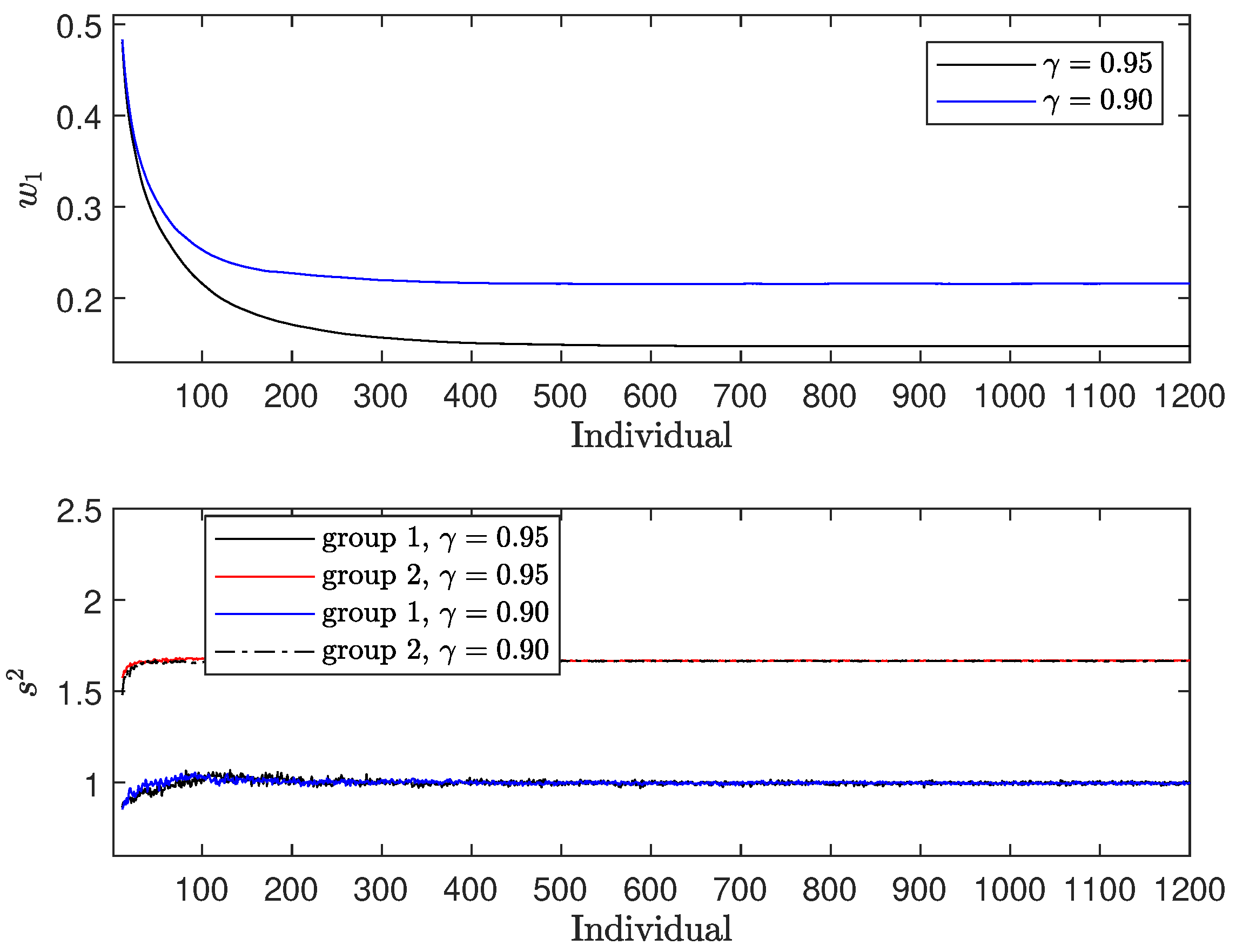
In the upper panel of Figure 1, we observe the fraction $w_1$, which represents the proportion of individuals allocated to treatment 1. Two distinct patterns emerge:

• Convergence below 0.5: $w_1$ converges to a value below 0.5 for both values of $\gamma$. This indicates that fewer individuals are allocated to the treatment with the lower average expectation, aligning with our intended allocation strategy;
• Overestimation of optimal allocation: The values of $w_1$ tend to overestimate the optimal allocation values obtained through the SDP approach, especially when considering an infinite sample size (as shown in Table 1, line 7 for I-R-optimal designs with $\gamma \in \{0.90,0.95\}$). This discrepancy arises primarily due to differences in expectation construction. In the SDP formulation, the expectation is established a priori using four points, whereas in the randomization procedure, it is adaptively constructed by considering the continuous design space of regressors for sampling. For example, the SDP-based optimal designs yield $w_1=0.0412$ for $\gamma =0.95$ and $w_1=0.1310$ for $\gamma =0.90$. In contrast, the adaptive design achieves $w_1=0.1491$ and $w_1=0.2163$ at convergence.

It is also observed that $w_1$ decreases as $\gamma$ increases, reflecting the increased weight given to the regret term. As a result, more individuals are allocated to the treatment with a higher expectation (treatment 2), despite its larger variance. The difference in allocation between the two treatments at convergence is 0.0728. In the lower panel of Figure 1, we examine the variance estimates $s_i^2$ for both treatments ($i\in ⟦I⟧$). Both estimates converge to the actual variance of the responses. Notably, $s_1^2$ shows more pronounced fluctuations, mainly because it is estimated from a smaller fraction of patients, whereas $s_2^2$ is estimated from the larger remaining fraction.

Figure 1. Results for $\gamma \in \{0.90,0.95\}$: (i) upper panel—$w_1$; (ii) lower panel—$s^2$.

Figure 1. Results for $\gamma \in \{0.90,0.95\}$: (i) upper panel—$w_1$; (ii) lower panel—$s^2$.

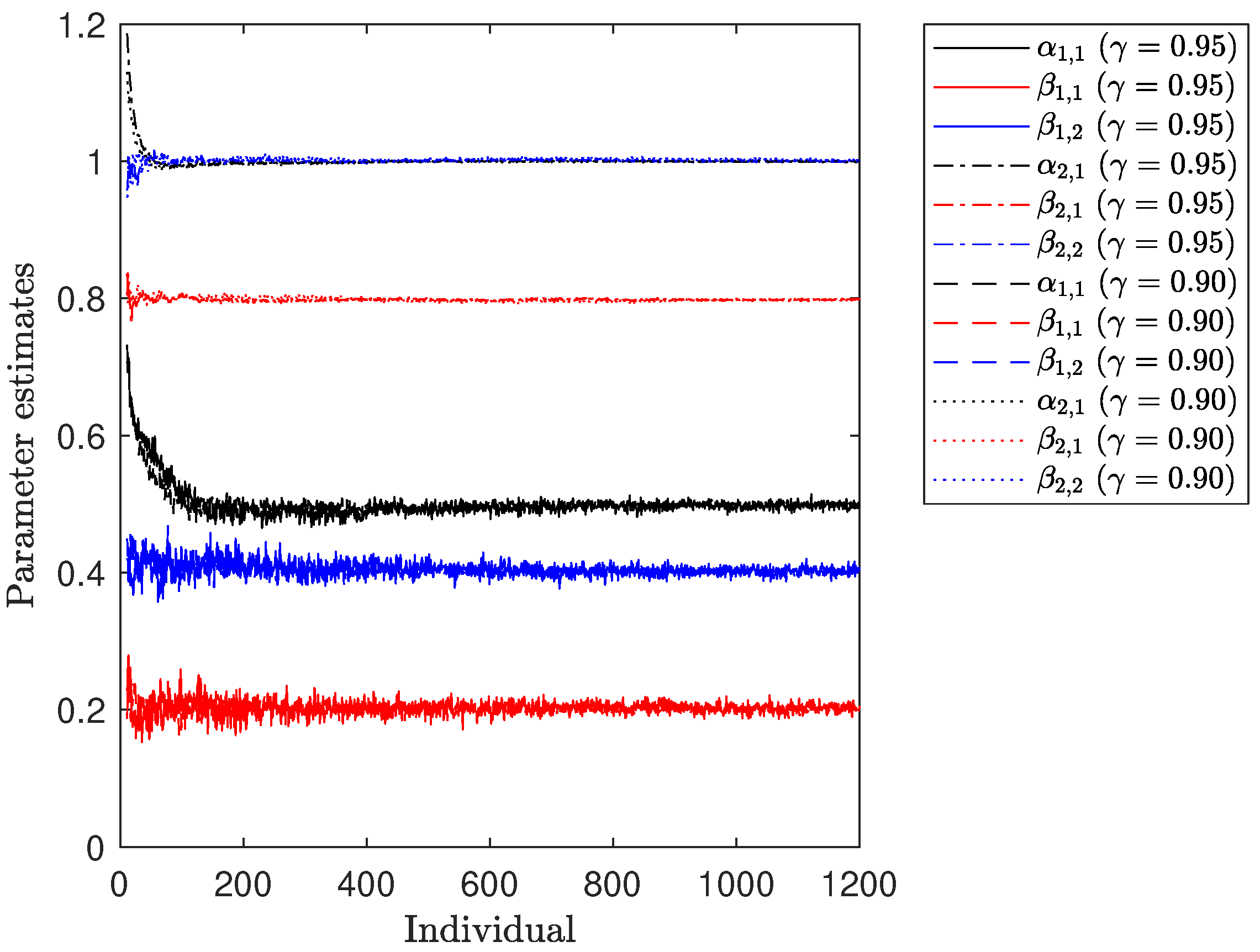
Figure 2 illustrates the progression of parameter estimates for both treatments over the course of the numerical experiment. It is noticeable that all of them converge towards the true values of $\mathit{\theta }$. However, a pattern resembling that observed for the variance estimates $s_i^2$ is also evident. Specifically, the estimation of the parameters for ${\eta }_1(\mathbf{x},\mathit{\theta })$ relies on a relatively small number of individuals, causing any new data point to have a more pronounced impact on the existing estimates. In contrast, the parameter estimates for ${\eta }_2(\mathbf{x},\mathit{\theta })$ exhibit smoother trajectories due to the larger number of responses considered in the fitting process.

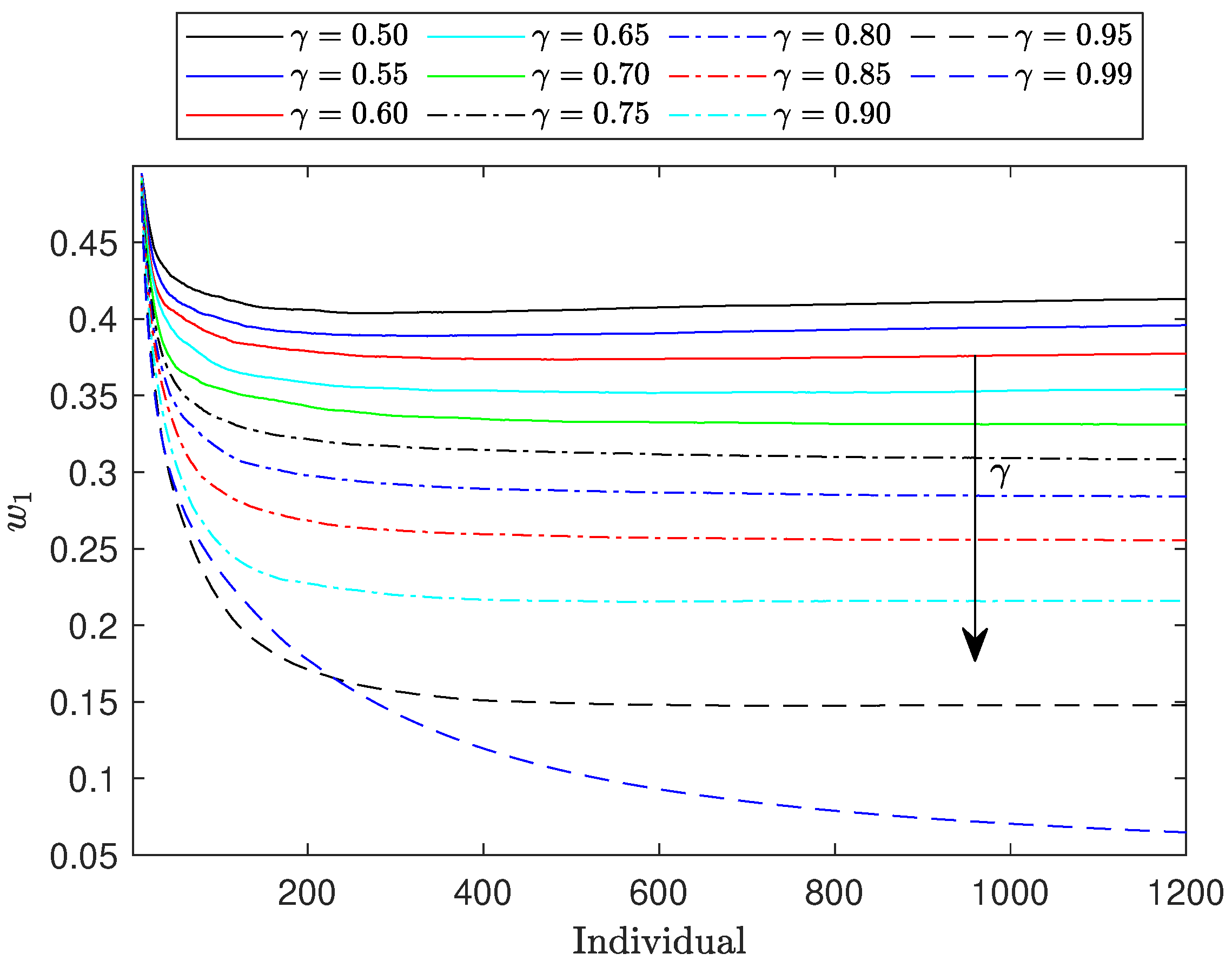
Figure 3 illustrates the evolution of $w_1$ across a range of $\gamma$ values from 0.50 to 0.99. The observed trends align with our expectations: as the weight assigned to the regret component increases, the values of $w_1$ decrease, and the corresponding curves become flatter. This downward trend in $w_1$ continues as $\gamma$ increases. Notably, when $\gamma$ reaches 1.0, corresponding to an allocation based solely on regret, $w_1$ approaches zero. Consequently, the Fisher information matrix (FIM) becomes nearly singular, and $det\left[M\right(\xi ,\mathit{\theta }\left)\right]$ approaches zero. This suggests that the information component of the objective function in Equation (8) becomes prone to numerical instability. This phenomenon occurs because when the FIM approaches singularity it becomes ill-conditioned, meaning its condition number increases significantly. This leads to numerical instability in the computation of its determinant, as small errors in the input data or round-off errors during calculations can result in large inaccuracies in the output.

To address these challenges while still evaluating the algorithm’s performance at extreme $\gamma$ values, we conducted tests with $\gamma =0.99$. The results remained consistent with the broader trends observed for other $\gamma$ values.

6. A Real Case Application

In this section, we apply the methodologies developed in Section 4 and Section 5 to a real-world case study. Specifically, we investigate the clinical trial described by Atkinson et al. [28], which focuses on the randomization of Parkinson’s disease patients. The primary aim of this study was to devise a randomization protocol for assigning patients to one of two treatment groups:

• Treatment 1: A novel procedure exploiting digital technologies.
• Treatment 2: A conventional treatment and monitoring approach.

To evaluate treatment efficacy, we use the quality of life (QoL) as the response variable. This is measured by the Parkinson’s Disease Questionnaire with 8 items (PDQ-8) [29], with QoL, denoted as $pdq8$, quantified as a percentage (ranging from 0% to 100%), where higher values indicate a lower quality of life. Several prognostic factors are known to influence QoL, with two demonstrating particularly strong correlations: (i) disease duration and stage, represented as $h\&q$, and measured on the Hoehn and Yahr scale [30,31]; and (ii) psychological well-being and neuropsychiatric symptoms (e.g., depression and anxiety), denoted as $bdi$, and assessed using Beck’s Depression Inventory (BDI) [32], based on responses to a structured questionnaire.

The models used for preliminary results for both treatments follow the structure outlined in Equation (1). The first prognostic factor, $x_1$, corresponds to $h\&q$, while the second, $x_2$, represents $bdi$. In the dataset used for modeling the two responses to these two variables $h\&q$ and $bdi$ are constrained to integer values. Specifically, $h\&q$ ranges from 1 to 5 (i.e., $h\&q\in [1,5]$), and $bdi$ ranges from 1 to 35 (i.e., $bdi\in [1,35]$). Consequently, the design space considered is denoted as $\mathbf{X}\equiv [1,5]\times [1,35]$, with covariate values randomly, but not uniformly, drawn from this space.

To mimic the empirical distribution of covariates we simulated from continuous distributions, which were then discretized. The variable $h\&q$ was generated by sampling from a normal distribution with a mean of 2.3837 and a standard deviation of 0.2857. Additionally, $bdi$ was sampled from a Gamma distribution with a shape parameter of 1.7678 and a scale parameter of 6.8145. These parameters were estimated from historical data. The model parameters for each treatment are specified as follows:

• For treatment 1: $({\alpha }_1,{\beta }_{1,1},{\beta }_{1,2})=(2.0941,3.9057,1.1089)$, with ${\sigma }_1^2=207.9267$.
• For treatment 2: $({\alpha }_2,{\beta }_{2,1},{\beta }_{2,2})=(-0.1015,4.1312,1.5117)$, with ${\sigma }_2^2=107.8993$.

The expected values for each model are (i) ${\mathbb{E}}_m\left[{\eta }_1(\mathbf{x},\mathit{\theta })\right]=33.7714$; and (ii) ${\mathbb{E}}_m\left[{\eta }_2(\mathbf{x},\mathit{\theta })\right]=39.5027$. Additionally, the values for ${\delta }_{min}$, $y_{{\mathrm{\Omega }}_m}^{max}$, and $∆$ are (i) $y_{{\mathrm{\Omega }}_m}^{min}={\delta }_{min}=5.5414$; (ii) $y_{{\mathrm{\Omega }}_m}^{max}=73.4640$; and (iii) $∆=67.9226$.

The D-optimal design is uniformly distributed, with $w_1=w_2=0.5000$. The normalization factor for the D-optimal design used, $det{\left[M({\xi }^{*},\mathit{\theta })\right]}^{1/\left[2\right(K+1\left)\right]}$, is 0.4203. It is important to note that given the characteristics of the response variable our objective is to minimize the second term in Equation (10), which is equivalent to maximizing its negative. Consequently, treatment 1 should be preferred due to its lower expectation, despite having a higher level of uncertainty. Visual inspection of the graphical representations of both models shows that in a specific region of the design space, defined as $\mathrm{\Omega }\equiv \left\{\right(h\&q,bdi)\in [1,5]\times [1,35]\mid 0.2251h\&q+0.4028bdi\le 2.1956\}$, where both $bdi$ and $h\&q$ are low, treatment 2 becomes the preferred choice.

The compound designs derived from the SDP formulation (9) for $\gamma =\{0.90,0.95\}$ are summarized in

Table 2. I-R-optimal designs for model (1) considering the response is $pdq8$ model ($w_2=1-w_1$).

${\mathit{\sigma }}_1^2$	${\mathit{\sigma }}_2^2$	I-R-Opt. Design †		I-R-Opt. Design ‡
		${\mathit{w}}_{\mathbf{1}}$	Opt	${\mathit{w}}_{\mathbf{1}}$	Opt
207.9267	107.8993	0.8120	−0.3711	0.6769	−0.3052

^† $\gamma =0.95$; ^‡ $\gamma =0.90$.

. These results align with the key trends identified in Section 4. Specifically, the treatment with the higher expectation is assigned to more than half of the individuals, despite also having a larger variance. This approach is consistent with our goal of maximizing the normalized regret. Notably, treatment 1 emerges as the most favorable option across almost the entire design domain. Moreover, as the weight of the regret component increases, the proportion of individuals allocated to treatment 1 also rises.

We now apply the treatment allocation algorithm discussed in Section 5 using the I-R rule. For this simulation, we set $n_s=2000$ and $P=1200$ (i.e., 1200 individuals). The values for $h\&q$ and $bdi$ are generated randomly from a uniform distribution over the ranges $[1,5]$ and $[1,35]$, respectively.

The upper panel of Figure 4 presents the weights $w_1$ for the two values of $\gamma$. These weights closely match the results obtained using SDP, as shown in Table 2. The difference in $w_1$ at convergence between $\gamma =0.90$ and $\gamma =0.95$ is approximately 0.0699. As expected, the weight assigned to treatment 1, which has the higher expectation, exceeds 0.5 in both cases, reaching around 0.80. This indicates that the allocation favors the treatment with the higher expectation.

The lower panel of Figure 4 displays the estimated variances of the response models for both treatment groups. The variances converge to a stable value, consistent with the test case. Notably, the group with the larger weight shows less variability in its variance estimate.

7. Conclusions

This paper demonstrates the application of compound design criteria for patient allocation in personalized medicine. Building upon the framework proposed in Duarte and Atkinson [2], which focused on patient allocation without considering ethical aspects, this study integrates ethical considerations into the allocation process. Specifically, the aim is to balance the acquisition of information for parametric response models with ethical considerations to ensure that each patient is assigned to the most effective available treatment.

The proposed approach is designed for response models that are linearly dependent on prognostic factors and characterized by continuous responses with distinct noise variances. A concave compound design criterion is developed that combines D-optimality with regret minimization, as detailed in Section 3. This dual criterion reflects the necessity of both maximizing the precision of parameter estimates and minimizing patient harm or regret, emphasizing the importance of fairness in clinical decision making, considering a weighted sum objective function.

To compute continuous optimal designs for the I-R criterion within a discrete design space, semidefinite programming is considered, as outlined in Section 4. Previous work in Duarte and Atkinson [2] addressed the numerical computation of designs maximizing information about parameters in a similar setup, and this paper builds upon those formulations. This work assumes that the variances of the treatments and model parameters are known, facilitating the construction of the expectation of each treatment response.

In scenarios where information about variances and model parameters is unavailable, a sequential adaptive optimal design algorithm is presented in Section 5. This algorithm iteratively updates estimates of parameters and variances as responses are collected. A systematic method for computing sequential adaptive optimal allocation schemes is proposed, and its application is illustrated with a concrete example. Although the approach aligns with reinforcement learning algorithms described in studies such as Zhao et al. [33] and Matsuura et al. [34], it differs by utilizing a known parametric structure a priori rather than a model-free representation.

The proposed computational methods are evaluated through two distinct scenarios: first, using a simplified illustrative example; and second, applying them to a real-world problem involving Parkinson’s disease patients. The treatments considered are (i) treatment 1, which employs a cutting-edge digital technology-centered procedure; and (ii) treatment 2, encompassing a traditional treatment and monitoring protocol.

Beyond computational efficiency, the proposed methods thoughtfully integrate ethical considerations into traditionally information-based designs in personalized medicine. This helps mitigate the ethical dilemma of balancing data collection in experimental settings with ensuring patients receive the best possible care. By incorporating regret minimization, the approach ensures that even patients not initially assigned to the optimal treatment experience reduced harm during the early stages of the experiment.

Moreover, this approach could be extended to non-medical domains such as marketing, economics, or policy-making, where optimal allocation strategies must balance information acquisition with fairness or ethical considerations. The framework’s flexibility also opens up the potential for application to treatments with binary or categorical outcomes, further broadening its relevance as well as models of linear and nonlinear classes.

The computational methods proposed are robust and versatile, offering practical insights into the allocation process. Future research could explore alternative randomization techniques, as discussed in Atkinson [25], which address trade-offs between efficiency losses due to randomization and bias reduction. Additionally, developing theoretical results to support the convergence of these methods would be beneficial. The approach introduced could also be adapted to models beyond the linear regression framework considered here, with careful attention to selecting appropriate regret measures and scaling for these alternative models.

Finally, while this study centers on known model parameters and variances, exploring scenarios with more complex model structures or unknown variance assumptions remains a promising direction. Introducing Bayesian methods or robust optimization techniques could offer a means of addressing the uncertainties inherent in patient responses or treatment variabilities. In particular, incorporating patient heterogeneity more explicitly into the model could further enhance the framework’s applicability to real-world clinical trials where patient responses may not follow identical parametric structures. The inclusion of such considerations could lead to even more refined and ethically sound allocation strategies, reinforcing the value of this approach in personalized medicine.