A Threshold Estimator for Ruin Probability Using the Fourier-Cosine Method in the Wiener–Poisson Risk Model

Abstract

In this paper, we propose a nonparametric estimator of ruin probability in the Wiener–Poisson risk model based on high-frequency data. The estimator is constructed via the Fourier-cosine method and the threshold technique, and the convergence rate is also studied for a large sample size. Finally, we verify the effectiveness of our estimator through some simulation studies.

1. Introduction

In the field of financial and actuarial mathematics, the study of ruin probability and related metrics has attracted significant attention from many researchers. In recent years, numerous notable results based on statistical inference have emerged regarding ruin probability and associated quantities. For example, see Shimizu [1], Zhang et al. [2], Zhang and Yang [3], Masiello [4], Zhang and Yang [5], and You et al. [6], among others.

Estimating ruin probability and related quantities in risk theory often involves employing various methods to develop estimators. Shimizu [1] applied the regularized Laplace inversion technique to estimate the Gerber–Shiu function in the Wiener–Poisson risk model. You and Cai [7] used the same technique to estimate ruin probability for a spectrally negative Lévy process. Zhang et al. [2] constructed an estimator of ruin probability using Fourier inversion and the kernel density estimation method in the classical risk model. Similarly, Zhang and Yang [3,5] developed estimators via Fourier inversion in a Lévy risk model. You et al. [6] established asymptotically normal distributions for the nonparametric estimator proposed by Zhang and Yang [5] in the classical risk model. Additionally, You and Gao [8] and You and Yin [9] applied threshold estimation and regularized Laplace inversion to obtain estimators for survival probability in the Wiener–Poisson risk model and the spectrally negative Lévy process, respectively. Gao and You [10] combined the threshold technique with Fourier inversion to estimate ruin probability under the tempered-stable Lévy subordinator. Zhang [11] estimated the Gerber–Shiu function using Fourier–Sinc series expansion in a compound Poisson risk model perturbed by diffusion. Zhang and Su [12] and Su et al. [13] used Laguerre series expansion to estimate the Gerber–Shiu function in the classical and perturbed compound Poisson models, respectively. Shimizu and Zhang [14] proposed an estimator for the Gerber–Shiu function by inverting a semiparametric estimator of its Fourier transform in a Lévy risk model. Yang et al. [15] applied the Fourier-cosine method to estimate the discounted density of the deficit at ruin in the classical risk model. Xie and Zhang [16] extended the Fourier-cosine method to estimate the expected present value of dividend payments before ruin and the expected discounted penalty function in the classical compound Poisson risk model under a constant barrier dividend strategy. Wang et al. [17] used the Fourier-cosine method to estimate the time value of ruin in a Lévy risk model.

More recently, the Fourier-cosine method has gained traction for estimating or approximating ruin probability and related quantities. Initially introduced by Fang and Oosterlee [18] for pricing European options, this method has since been extended to ruin theory. Chau et al. [19] approximated infinite-time ruin probability using the Fourier-cosine method under a Lévy subordinator model. In a subsequent study, Chau et al. [20] systematically examined the approximation of Gerber–Shiu functions using this method. Zhang [21] applied the Fourier-cosine method to approximate the density of time to ruin in the classical compound Poisson risk model. Lee et al. [22] incorporated the Fourier-cosine method to estimate finite-time ruin probability in a Lévy process. Li et al. [23] extended Lee et al.’s work to approximate Gerber–Shiu functions in a Lévy process. In addition to these approaches, Wang and Zhang [24] approximated the Gerber–Shiu function using frame duality projection in a Lévy risk model. In our work, we adopt the Fourier-cosine method to estimate ruin probability.

In finance, high-frequency trading generates vast amounts of data suitable for statistical analysis, offering insights into market dynamics. Ruin probability research is crucial for managing specialized funds that prioritize long-term sustainability over short-term gains. These funds aim to maintain consistent spending levels and avoid financial ruin, thereby improving their long-term survival. For related studies, see Karathanasopoulos et al. [25]. Shimizu and Zhang [14] discussed the application of high-frequency observation schemes in financial statistics and insurance.

In our work, we assume that the high-frequency data consist of $n+1$ discrete-time observations of the surplus process (1) with time steps, i.e., the discrete sample $X^n=\{X_{t_m^n},m=0,1,2,\dots ,n\}$, $t_m^n=m{h}_n(m=0,1,2,\dots ,n)$. The asymptotic framework assumes that $n{h}_n\to \infty$ and $h_n\to 0$ while $n\to \infty$. This high-frequency assumption is frequently employed in statistical inference for Lévy processes. See, for example, Shimizu [26], Zhang and Yang [3], and Comte and Genon-Catalot [27,28]. Under this assumption, we obtain observable data on the surplus process, though we remain uncertain about the occurrence of jumps within the small intervals $(t_{m-1}^n,t_m^n]$ which can significantly affect the accuracy of our ruin probability estimator. Therefore, we must devise a method to use observable data to detect whether jumps occurred within these small intervals. Mancini [29], You and Gao [8], Gao and You [10], and Shimizu [26] employed a threshold technique to identify jumps whose sizes exceed a defined threshold function. Given discrete observations, this technique helps differentiate between fluctuations due to diffusion shocks and those caused by jumps.

In this paper, we propose an estimator for ruin probability using the threshold technique and the Fourier-cosine method. By integrating the threshold technique with the Fourier-cosine method, the estimator becomes more stable and reliable, improving its accuracy in assessing ruin probability.

The remainder of this paper is organized as follows: In Section 2, we introduce the risk model, assumptions, ruin probability, and its Fourier transform. Section 3 presents several estimators based on the Fourier-cosine method and the threshold technique. Section 4 establishes the asymptotic properties of our estimators and provides technical proofs. Section 5 demonstrates the effectiveness of our estimators through simulations. Finally, we provide concluding remarks in Section 6.

2. Preliminaries

2.1. Risk Model and Some Assumptions

The Wiener–Poisson risk process is defined by

$$X_t=x+ct+\sigma W_t-\sum _{j=1}^{N_t}{U}_j,t\ge 0,$$

(1)

where $x\ge 0$ is the initial surplus level, $c>0$ is a parameter, $\sigma >0$ is the diffusion coefficient, $\{W_t,t\ge 0\}$ is a standard Wiener process, $\{N_t,t\ge 0\}$ is a Poisson process with intensity $\lambda >0$, and $U_1,U_2,U_3,\dots$ comprise an independent and identically distributed positive sequence of random variables with the common distribution F(density f). Suppose that $\{N_t,t\ge 0\}$, $\{W_t,t\ge 0\}$, and $\{U_j,j=1,2,\dots \}$ are independent of each other.

In this paper, we assume that the Poisson intensity $\lambda$, the distribution function F, and diffusion coefficient $\sigma$ are unknown. In this case, our objective is to estimate the ruin probability of risk process (1).

Next, we make some assumptions for our theoretical results:

Let ${\mu }_n={\int }_0^{\infty }{x}^{n}F\left(dx\right)$, $n=1,2,3,\dots$.

Assumption A1. 

${\mu }_n<\infty$, $n=1,2,4$.

Assumption A2. 

The safety loading condition holds, i.e., $c>\lambda {\mu }_1$.

2.2. Ruin Probability and Its Fourier Transform

Let $\tau =inf\{t\ge 0:X_t\le 0\}$. The infinite-time horizon ruin probability is given by

$$\begin{array}{c}\hfill \Psi \left(x\right)=\mathbf{P}\left(\tau <\infty |X_0=x\right),x\ge 0.\end{array}$$

(2)

Let $\vartheta \left(s\right)$ be the characteristic exponent of $X_t-x$ defined by $\vartheta \left(s\right):=t^{-1}logE\left[e^{is(X_t-x)}\right]$, which is easily calculated by the independent property of $W,N,U_j$ as follows:

$$\begin{array}{c}\hfill \vartheta \left(s\right)=ics-{\displaystyle \frac{{\sigma }^2}{2}}{s}^2+\lambda \left({\int }_0^{\infty }{e}^{-isx}F\left(dx\right)-1\right).\end{array}$$

(3)

With reference to Zhang and Yang [5] and Gao and You [10], the Fourier transform of $\Psi \left(x\right)$ is given by

$$\begin{array}{ccc}\hfill \mathcal{F}\Psi \left(s\right)& =& {\displaystyle \frac{\frac{{\sigma }^2}{2}is+\frac{\lambda }{is}{\int }_0^{\infty }(e^{isx}-1)F\left(dx\right)-\lambda {\mu }_1}{ics+\frac{{\sigma }^2}{2}{s}^2-\lambda {\int }_0^{\infty }(e^{isx}-1)F\left(dx\right)}}\hfill \end{array}$$

(4)

$$\begin{array}{ccc}& =& {\displaystyle \frac{\vartheta (-s)+ics[1-\rho ]}{-is\vartheta (-s)}}.\hspace{1em}\hspace{1em}\hspace{1em}\hspace{1em}\hfill \end{array}$$

(5)

where $\rho ={\displaystyle \frac{\lambda {\mu }_1}{c}}$ and $\vartheta (-s)=-ics-{\displaystyle \frac{{\sigma }^2}{2}}{s}^2+\lambda \left({\int }_0^{\infty }{e}^{isx}F\left(dx\right)-1\right)$. By (4) and

$$\begin{array}{c}\hfill \underset{s\to 0}{lim}{\displaystyle \frac{1}{is}}{\int }_0^{\infty }(e^{isx}-1)F\left(dx\right)={\int }_0^{\infty }\underset{s\to 0}{lim}{\displaystyle \frac{(e^{isx}-1)}{is}}F\left(dx\right)={\mu }_1,\\ \hfill \underset{s\to 0}{lim}{\displaystyle \frac{1}{{\left(is\right)}^2}}{\int }_0^{\infty }(e^{isx}-1-isx)F\left(dx\right)={\int }_0^{\infty }\underset{s\to 0}{lim}{\displaystyle \frac{(e^{isx}-1-isx)}{{\left(is\right)}^2}}F\left(dx\right)={\displaystyle \frac{{\mu }_2}{2}},\end{array}$$

and Equation (5) yields that

$$\begin{array}{cc}\hfill \mathcal{F}\Psi \left(s\right)& =\left\{\begin{array}{cc}{\displaystyle \frac{\vartheta (-s)+ics(1-\rho )}{-is\vartheta (-s)}},\hfill & s\ne 0,\hfill \\ \\ {\displaystyle \frac{\frac{{\sigma }^2}{2}+\frac{\lambda {\mu }_2}{2}}{c-\lambda {\mu }_1}},\hfill & s=0.\hfill \end{array}\right.\hfill \end{array}$$

(6)

3. Estimation of Ruin Probability

In this section, our aim is to construct an estimator for $\Psi \left(x\right)$ using the sample $X^n$.

Let us denote by $Z_m$ the increment $X_{t_m^n}-X_{t_{m-1}^n}$ for $m=1,\dots ,n$. $h_n$ is the sampling interval, denoted by $t_m^n-t_{m-1}^n$.

If we can estimate $\lambda {\mu }_1$, $\lambda {\mu }_2$, ${\sigma }^2$, $\rho$, and $\vartheta \left(s\right)$ in (6), then $\mathcal{F}\Psi \left(s\right)$ can be estimated with the plug-in device. Inspired by Zhang and Yang [3,5] and Gao and You [10], let us denote $\psi \left(s\right)$ = $E\left[e^{is{Z}_1}\right]$, an estimator of $\vartheta \left(s\right)$, which is given by

$$\begin{array}{c}\hfill \widehat{\vartheta }\left(s\right)={\displaystyle \frac{1}{h_n}}\left(\widehat{\psi }\left(s\right)-1\right),\end{array}$$

(7)

where

$$\begin{array}{c}\hfill \widehat{\psi }\left(s\right)={\displaystyle \frac{1}{n}}\sum _{m=1}^n{e}^{is{Z}_m}\end{array}$$

is an empirical-type estimator of $\psi \left(s\right)$.

3.1. Threshold Function Technique

Inspired by Shimizu [26], Mancini [29], and You and Gao [7], we introduce the filter

$$\begin{array}{c}\hfill {\mathcal{D}}_m^n:=\left\{\omega \in \Omega :c{h}_n-Z_m>r_n\right\},\end{array}$$

(8)

where $r_n=h_n^{\theta }>0$ is a suitable threshold function dependent on n such that ${lim}_{n\to \infty }{r}_n=0$ and $\theta$ is a positive constant. Let ${\mathcal{C}}_m^n$ := $\left\{\omega \in \Omega :c{h}_n-Z_m\le r_n\right\}$ be the complement of ${\mathcal{D}}_m^n$.

The function $r_n$, suitably chosen, plays the role of a threshold to detect the existence of a jump in each sampling interval. Given these filters and $r_n$, we can observe that there is no jump in the interval $\left(t_{m-1}^n,t_m^n\right]$ if $c{h}_n-Z_m\le r_n$.

By Mancini [29] and You and Gao [8], the natural estimators for $\lambda {\mu }_1$ and ${\sigma }^2$ are, respectively, given by

$$\begin{array}{c}\hfill \widehat{\lambda {\mu }_1}={\displaystyle \frac{{\sum }_{m=1}^n(c{h}_n-Z_m){\mathbf{I}}_{{\mathcal{D}}_m^n}}{n{h}_n}},\widehat{{\sigma }^2}={\displaystyle \frac{1}{n{h}_n}}\sum _{m=1}^n{(c{h}_n-Z_m)}^2{\mathbf{I}}_{{\mathcal{C}}_m^n}.\end{array}$$

(9)

By Equation (9) and $\rho ={\displaystyle \frac{\lambda {\mu }_1}{c}}$, an estimator of $\rho$ is given by

$$\begin{array}{c}\hfill \widehat{\rho }={\displaystyle \frac{\widehat{\lambda {\mu }_1}}{c}}={\displaystyle \frac{1}{c}}{\displaystyle \frac{{\sum }_{m=1}^n(c{h}_n-Z_m){\mathbf{I}}_{{\mathcal{D}}_m^n}}{n{h}_n}}.\end{array}$$

(10)

According to Remark 3 in Wang et al. [17], we construct an estimator of $\lambda {\mu }_2$ as follows:

$$\begin{array}{c}\hfill \widehat{\lambda {\mu }_2}={\displaystyle \frac{1}{n{h}_n}}\sum _{m=1}^n{\left(Z_m-c{h}_n\right)}^2-h_n{\left(\widehat{\lambda {\mu }_1}\right)}^2-\widehat{{\sigma }^2}.\end{array}$$

(11)

Combining Equations (6), (7), (9), (10) and (11), we estimate $\mathcal{F}\Psi \left(s\right)$ by

$$\begin{array}{cc}\hfill \widehat{\mathcal{F}\Psi }\left(s\right)& =\left\{\begin{array}{cc}{\displaystyle \frac{\widehat{\vartheta }(-s)+ics(1-\widehat{\rho })}{-is\widehat{\vartheta }(-s)}},\hfill & s\ne 0,\hfill \\ \\ {\displaystyle \frac{\frac{\widehat{{\sigma }^2}}{2}+\frac{\widehat{\lambda {\mu }_2}}{2}}{c-\widehat{\lambda {\mu }_1}}},\hfill & s=0.\hfill \end{array}\right.\hfill \end{array}$$

(12)

3.2. Fourier-Cosine Method

To ensure the smooth comprehension of the paper, we will provide a revised introduction to the Fourier-cosine method.

For an integrable function $f\left(x\right)$, $x\in [a_1,a_2]$, it has the following cosine series expansion,

$$\begin{array}{c}\hfill f\left(x\right)=\underset{k=0}{\overset{\infty }{{\sum }^{\prime }}}{\mathcal{A}}_{f,k}cos(k\pi {\displaystyle \frac{x-a_1}{a_2-a_1}}),\end{array}$$

where ${\sum }^{\prime }$ indicates that the first term in the summation is weighted by one-half, and the cosine coefficients are given by

$$\begin{array}{c}\hfill {\mathcal{A}}_{f,k}={\displaystyle \frac{2}{a_2-a_1}}\Re \left\{{\int }_{a_1}^{a_2}f\left(x\right)exp(ik\pi {\displaystyle \frac{x-a_1}{a_2-a_1}})dx\right\},k=0,1,2,\dots ,\end{array}$$

where ℜ means taking the real part and $i=\sqrt{-1}$ is the imaginary unit.

Let $a_1=0$ and $a_2=a$, after choosing large a, we have

$$\begin{array}{c}\hfill A_{f,k}\approx B_{f,k}:={\displaystyle \frac{2}{a}}·\Re \left\{\mathcal{F}f(k\pi /a)\right\}={\displaystyle \frac{2}{a}}·\Re \left\{{\int }_0^{a}f\left(x\right)exp(ik\pi {\displaystyle \frac{x}{a}})dx\right\},k=0,1,2,\dots ,\end{array}$$

then we obtain the following Fourier-cosine approximation for $f\left(x\right)$,

$$\begin{array}{c}\hfill f\left(x\right)\approx \underset{k=0}{\overset{\infty }{{\sum }^{\prime }}}{B}_{f,k}cos(k\pi {\displaystyle \frac{x}{a}})\approx \tilde{f}\left(x\right):=\underset{k=0}{\overset{K}{{\sum }^{\prime }}}{B}_{f,k}cos(k\pi {\displaystyle \frac{x}{a}}),0\le x\le a,\end{array}$$

(13)

where K is a larger integer applied to truncate the infinite series.

By the Fourier-cosine approximation in (13), we can approximate $\Psi \left(x\right)$ as follows:

$$\begin{array}{c}\hfill \Psi \left(x\right)\approx \tilde{\Psi }\left(x\right):=\underset{k=0}{\overset{K}{{\sum }^{\prime }}}{B}_{\Psi ,k}cos(k\pi {\displaystyle \frac{x}{a}}),0\le x\le a,\end{array}$$

(14)

where $B_{\Psi ,k}={\displaystyle \frac{2}{a}}·\Re \left\{\mathcal{F}\Psi \left({\displaystyle \frac{k\pi }{a}}\right)\right\},k=0,1,\dots .$.

Therefore, by (12) and (14), we can obtain the estimator of $\Psi \left(x\right)$ as follows:

$$\begin{array}{c}\hfill \widehat{\Psi }\left(x\right):=\underset{k=0}{\overset{K}{{\sum }^{\prime }}}{\widehat{B}}_{\Psi ,k}cos(k\pi {\displaystyle \frac{x}{a}}),0\le x\le a,\end{array}$$

(15)

where ${\widehat{B}}_{\Psi ,k}={\displaystyle \frac{2}{a}}·\Re \left\{\widehat{\mathcal{F}\Psi }\left({\displaystyle \frac{k\pi }{a}}\right)\right\},k=0,1,\dots .$.

4. Asymptotic Properties of Estimators

In this section, we investigate the asymptotic properties of $\widehat{\mathcal{F}\Psi }\left(s\right)$ and $\widehat{\Psi }\left(x\right)$. To begin, we need to examine the asymptotic properties of $\widehat{{\sigma }^2}$, $\widehat{\rho }$, $\widehat{\vartheta }\left(s\right)$, and $\widehat{\lambda {\mu }_2}$. For the ease of exposure, we firstly introduce some notation. Symbols $\stackrel{\mathbf{P}}{\to }$ and $\stackrel{\mathbf{D}}{\to }$ stand for the convergence in probability and in distribution, respectively. Define the set $\mathcal{S}:=\left\{k\pi /a:k=0,1,\dots ,K\right\}$.

The following Lemma 1 gives the rate of convergence of $\widehat{{\sigma }^2}$.

Lemma 1. 

Let $r_n=h_n^{\theta }$ with $\theta \in (0,{\displaystyle \frac{1}{2}})$. Suppose that $n{h}_n\to \infty$, $n{h}_n^2\to 0$, and $h_n\to 0$ as $n\to \infty$, then

$$\begin{array}{c}\widehat{{\sigma }^2}\stackrel{\mathbf{P}}{\to }{\sigma }^2,n\to \infty ,\\ \sqrt{n}(\widehat{{\sigma }^2}-{\sigma }^2)\stackrel{\mathbf{D}}{\to }\mathcal{N}\left(0,2{\sigma }^4\right),n\to \infty .\end{array}$$

(16)

Proof. 

The proof of Lemma 1 is easily obtained by Appendix A in You and Gao [8]. □

Lemma 2. 

Under Assumptions 1 and 2, if $\theta \in (0,{\displaystyle \frac{1}{2}})$, $n{h}_n\to \infty$, $n{h}_n^{1+\alpha }\to 0$ for some $\alpha \in \left(0,1\right]$ and $h_n\to 0$ as $n\to \infty$. Then,

$$\begin{array}{c}\hfill \widehat{\rho }-\rho =O_P({\displaystyle \frac{1}{\sqrt{n{h}_n}}}).\end{array}$$

(17)

Proof. 

It is easy to obtain Equation (17) by the proof of Theorem 1 in You and Yin [9]. □

Lemma 3. 

Suppose that $h_n\to 0$, $n{h}_n\to \infty$ as $n\to \infty$, we have

$$\begin{array}{c}\widehat{\vartheta }\left(s\right)\stackrel{\mathbf{P}}{\to }\vartheta \left(s\right),\\ \sqrt{n{h}_n}(\widehat{\vartheta }\left(s\right)-\vartheta \left(s\right))\stackrel{\mathbf{D}}{\to }\mathcal{N}(0,\vartheta \left(2s\right)-2\vartheta \left(s\right)).\end{array}$$

(18)

Proof. 

Referring to the proof of Theorem 4.4 in You and Cai [7], we can easily obtain the result. □

Lemma 4. 

For real-valued integrable function f supported on $[0,\infty )$, suppose that $|f^{\prime }(0+)|<\infty$, $|f^{\prime }\left(a\right)|<\infty$, and ${\int }_0^{\infty }\left|f^{″}\left(y\right)\right|dy<\infty$. Then for some positive constants $c_1$ and $c_2$, we have

$$\begin{array}{c}\hfill \underset{x\in [0,a]}{sup}|f\left(x\right)-\tilde{f}\left(x\right)|\le c_{1}a{K}^{-1}+c_{2}K{a}^{-1}{\int }_a^{\infty }\left|f\left(y\right)\right|dy.\end{array}$$

Proof. 

The proof of Lemma 4 can be referenced from Appendix A in Xie and Zhang [16]. □

Proposition 1. 

Under Assumptions 1 and 2, suppose that $h_n\to 0$, $n{h}_n\to \infty$ as $n\to \infty$, and we have

$$\begin{array}{c}\hfill \sqrt{n{h}_n}\left({\displaystyle \frac{1}{n}}\sum _{m=1}^n{\displaystyle \frac{{\left(Z_m-c{h}_n\right)}^2}{h_n}}-({\sigma }^2+\lambda {\mu }_2)\right)\stackrel{\mathbf{D}}{\to }\mathcal{N}(0,\lambda {\mu }_4).\end{array}$$

(19)

Proof. 

Firstly, according to the law of large numbers, we have

$$\begin{array}{c}\hfill {\displaystyle \frac{1}{n}}\sum _{m=1}^n{\displaystyle \frac{{\left(Z_m-c{h}_n\right)}^2}{h_n}}\stackrel{\mathbf{P}}{\to }{\sigma }^2+\lambda {\mu }_2,n\to \infty .\end{array}$$

Because of the stationary and independent increments of the risk process (1), we have

$$\begin{array}{ccc}\hfill & & \underset{n\to \infty }{lim}\mathbf{Var}\left(\sqrt{n{h}_n}\left({\displaystyle \frac{1}{n}}\sum _{m=1}^n{\displaystyle \frac{{\left(Z_m-c{h}_n\right)}^2}{h_n}}\right)\right)\hfill \\ & =& \underset{n\to \infty }{lim}{\displaystyle \frac{1}{h_n}}\mathbf{Var}\left({\left(Z_m-c{h}_n\right)}^2\right)\hfill \\ & =& \lambda {\mu }_4.\hfill \end{array}$$

(20)

Through the central limit theorem, we obtain the result. □

Proposition 2. 

Assuming the same conditions as in Lemma 2, we have

$$\begin{array}{c}\hfill \widehat{\lambda {\mu }_2}-\lambda {\mu }_2=O_P\left({\displaystyle \frac{1}{\sqrt{n{h}_n}}}\right).\end{array}$$

(21)

Proof. 

By Equation (11), we can obtain

$$\begin{array}{ccc}\hfill \widehat{\lambda {\mu }_2}-\lambda {\mu }_2& =& {\displaystyle \frac{1}{n}}\sum _{m=1}^n{\displaystyle \frac{{\left(Z_m-c{h}_n\right)}^2}{h_n}}-{\displaystyle \frac{1}{h_n}}\left(E[Z_m-c{h}_n]\right)\hfill \\ & & -h_n(\widehat{\lambda {\mu }_1}+\lambda {\mu }_1)(\widehat{\lambda {\mu }_1}-\lambda {\mu }_1)\hfill \\ & & -(\widehat{{\sigma }^2}-{\sigma }^2).\hfill \end{array}$$

Combining Lemmas 1 and 2 with Proposition 1, we can obtain

$$\begin{array}{c}\hfill \widehat{\lambda {\mu }_2}-\lambda {\mu }_2=O_P\left({\displaystyle \frac{1}{\sqrt{n{h}_n}}}\right).\end{array}$$

□

Theorem 1. 

Assuming the same conditions as in Lemma 2, we have

$$\begin{array}{c}\hfill \widehat{\mathcal{F}\Psi }\left(s\right)-\mathcal{F}\Psi \left(s\right)=O_P\left({\displaystyle \frac{1}{\sqrt{n{h}_n}}}\right).\end{array}$$

(22)

Proof. 

First, let us consider the case where $s=0$. By (12), we have

$$\begin{array}{ccc}\hfill \widehat{\mathcal{F}\Psi }\left(0\right)-\mathcal{F}\Psi \left(0\right)& =& {\displaystyle \frac{\frac{\widehat{{\sigma }^2}}{2}+\frac{\widehat{\lambda {\mu }_2}}{2}}{c-\widehat{\lambda {\mu }_1}}}-{\displaystyle \frac{\frac{{\sigma }^2}{2}+\frac{\lambda {\mu }_2}{2}}{c-\lambda {\mu }_1}}\hfill \\ & =& {\displaystyle \frac{(\widehat{{\sigma }^2}-{\sigma }^2)+(\widehat{\lambda {\mu }_2}-\lambda {\mu }_2)}{2(c-\lambda {\mu }_1)}}\hfill \\ & & +{\displaystyle \frac{\widehat{{\sigma }^2}+\widehat{\lambda {\mu }_2}}{2(c-\widehat{\lambda {\mu }_1})(c-\lambda {\mu }_1)}}·(\widehat{\lambda {\mu }_1}-\lambda {\mu }_1).\hfill \end{array}$$

By Lemmas 1 and 2 and Equation (21), we can establish that

$$\begin{array}{c}\hfill \widehat{\mathcal{F}\Psi }\left(0\right)-\mathcal{F}\Psi \left(0\right)=O_P\left({\displaystyle \frac{1}{\sqrt{n{h}_n}}}\right).\end{array}$$

(23)

If $s\ne 0$, we have

$$\begin{array}{ccc}\hfill \widehat{\mathcal{F}\Psi }\left(s\right)-\mathcal{F}\Psi \left(s\right)& =& {\displaystyle \frac{\widehat{\vartheta }(-s)+ics(1-\widehat{\rho })}{-is\widehat{\vartheta }(-s)}}-{\displaystyle \frac{\vartheta (-s)+ics(1-\rho )}{-is\vartheta (-s)}}\hfill \\ & =& {\displaystyle \frac{(1-\rho )\left(\widehat{\vartheta }(-s)-\vartheta (-s)\right)+\vartheta (-s)\left(\widehat{\rho }-\rho \right)}{{\displaystyle \frac{1}{c}}\vartheta (-s)\widehat{\vartheta }(-s)}}.\hfill \end{array}$$

Moreover, by Lemmas 2 and 3, we have

$$\begin{array}{c}\hfill \widehat{\mathcal{F}\Psi }\left(s\right)-\mathcal{F}\Psi \left(s\right)=O_P\left({\displaystyle \frac{1}{\sqrt{n{h}_n}}}\right),s\ne 0.\end{array}$$

(24)

Finally, combining Equations (23) and (24), we have

$$\begin{array}{c}\hfill \widehat{\mathcal{F}\Psi }\left(s\right)-\mathcal{F}\Psi \left(s\right)=O_P\left({\displaystyle \frac{1}{\sqrt{n{h}_n}}}\right).\end{array}$$

□

Remark 1. 

For $s\ne 0$, by Equations (7) and (10) and Lemma 3, we have

$$\begin{array}{cc}\hfill \sqrt{n{h}_n}(\widehat{\mathcal{F}\Psi }\left(s\right)-\mathcal{F}\Psi \left(s\right))=& \sqrt{n{h}_n}{\displaystyle \frac{1}{n}}\sum _{m=1}^n\left[{\displaystyle \frac{\left[\left(c-\lambda {\mu }_1\right)\left(e^{-is{Z}_m}-1\right)+\vartheta (-s)\left(c{h}_n-Z_m\right){\mathbf{I}}_{{\mathcal{D}}_m^n}\right]}{h_n{\vartheta }^2(-s)}}\right.\hfill \\ \hfill & \left.-{\displaystyle \frac{c}{\vartheta (-s)}}\right]+o_P\left(1\right).\hfill \end{array}$$

By the Theorem 1 in Mancini [29] and the central limit theorem, we obtain that

$$\begin{array}{c}\hfill \sqrt{n{h}_n}(\widehat{\mathcal{F}\Psi }\left(s\right)-\mathcal{F}\Psi \left(s\right))\stackrel{\mathrm{D}}{\to }\mathcal{N}(0,S),\end{array}$$

(25)

where

$$\begin{array}{c}\hfill S={\displaystyle \frac{{\left(c-\lambda {\mu }_1\right)}^2(\vartheta (-2s)-2\vartheta (-s))}{{\vartheta }^4(-s)}}-{\displaystyle \frac{2\lambda \left(c-\lambda {\mu }_1\right)\left({\int }_0^{\infty }x{e}^{isx}F\left(dx\right)-{\mu }_1\right)}{{\vartheta }^3(-s)}}+{\displaystyle \frac{\lambda {\mu }_2}{{\vartheta }^2(-s)}}.\end{array}$$

In Zhang and Yang [3] and You and Cai [7], they gave an estimator of ρ as follows:

$$\begin{array}{c}\hfill {\widehat{\rho }}^{*}={\displaystyle \frac{1}{cn{h}_n}}\sum _{m=1}^n\left(c{h}_n-Z_m\right).\end{array}$$

(26)

By Theorem 4.1 in You and Cai [7],

$$\begin{array}{c}\hfill \sqrt{n{h}_n}\left({\widehat{\rho }}^{*}-\rho \right)\stackrel{\mathrm{D}}{\to }\mathcal{N}\left(0,{\displaystyle \frac{{\sigma }^2+\lambda {\mu }_2}{c^2}}\right).\end{array}$$

(27)

If we replace $\widehat{\rho }$ with ${\widehat{\rho }}^{*}$ in (28), the estimator of $\mathcal{F}\Psi \left(s\right)$ is

$$\begin{array}{cc}\hfill {\widehat{\mathcal{F}\Psi }}^{*}\left(s\right)& =\left\{\begin{array}{cc}{\displaystyle \frac{\widehat{\vartheta }(-s)+ics(1-{\widehat{\rho }}^{*})}{-is\widehat{\vartheta }(-s)}},\hfill & s\ne 0,\hfill \\ \\ {\displaystyle \frac{\frac{\widehat{{\sigma }^2}}{2c}+\frac{\widehat{\lambda {\mu }_2}}{2c}}{1-{\widehat{\rho }}^{*}}},\hfill & s=0.\hfill \end{array}\right.\hfill \end{array}$$

(28)

By the central limit theorem,

$$\begin{array}{c}\hfill \sqrt{n{h}_n}\left({\widehat{\mathcal{F}\Psi }}^{*}\left(s\right)-\mathcal{F}\Psi \left(s\right)\right)\stackrel{\mathrm{D}}{\to }\mathcal{N}\left(0,S^{*}\right)\end{array}$$

(29)

where

$$\begin{array}{cc}\hfill S^{*}& ={\displaystyle \frac{{\left(c-\lambda {\mu }_1\right)}^2(\vartheta (-2s)-2\vartheta (-s))}{{\vartheta }^4(-s)}}+{\displaystyle \frac{\lambda {\mu }_2+{\sigma }^2}{{\vartheta }^2(-s)}}\hfill \\ \hfill & +{\displaystyle \frac{2\left(c-\lambda {\mu }_1\right)\left(is{\sigma }^2+\lambda {\int }_0^{\infty }x{e}^{isx}F\left(dx\right)-\lambda {\mu }_1\right)}{{\vartheta }^3(-s)}}.\hfill \end{array}$$

(30)

Comparing ${\widehat{\mathcal{F}\Psi }}^{*}\left(s\right)$ to $\widehat{\mathcal{F}\Psi }\left(s\right)$, we can easily see that $\Re \left\{S^{*}\right\}$ is greater than $\Re \left\{S\right\}$. Therefore, we can know that our estimator $\widehat{\mathcal{F}\Psi }\left(s\right)$ works better.

Theorem 2. 

Assuming the same conditions as in Lemma 2, we have

$$\begin{array}{c}\hfill \underset{0\le x\le a}{sup}\left|\widehat{\Psi }\left(x\right)-\tilde{\Psi }\left(x\right)\right|=O_P\left({\displaystyle \frac{1}{\sqrt{n{h}_n}}}\right).\end{array}$$

(31)

Proof. 

Firstly, by Equations (14) and (15), we obtain

$$\begin{array}{c}\hfill \widehat{\Psi }\left(x\right)-\tilde{\Psi }\left(x\right)=\underset{k=0}{\overset{K}{{\sum }^{\prime }}}[{\widehat{B}}_{\Psi ,k}-{\tilde{B}}_{\Psi ,k}]cos(k\pi {\displaystyle \frac{x}{a}}),0\le x\le a,\end{array}$$

which gives

$$\begin{array}{c}\hfill \underset{0\le x\le a}{sup}\left|\widehat{\Psi }(x)-\tilde{\Psi }(x)\right|\le \sum _{k=0}^K\left|{\widehat{B}}_{\Psi ,k}-{\tilde{B}}_{\Psi ,k}\right|\le (K+1)·\underset{k=0,1,\dots ,K}{sup}\left|{\widehat{B}}_{\Psi ,k}-{\tilde{B}}_{\Psi ,k}\right|.\end{array}$$

(32)

Next, we derive the convergence rate of ${\widehat{B}}_{\Psi ,k}$. For each integer k, we have

$$\begin{array}{c}\hfill \left|{\widehat{B}}_{\Psi ,k}-{\tilde{B}}_{\Psi ,k}\right|=\left|{\displaystyle \frac{2}{a}}·\Re \left\{\widehat{\mathcal{F}\Psi }\left({\displaystyle \frac{k\pi }{a}}\right)\right\}-{\displaystyle \frac{2}{a}}·\Re \left\{\mathcal{F}\Psi \left({\displaystyle \frac{k\pi }{a}}\right)\right\}\right|\le {\displaystyle \frac{2}{a}}·\left|\widehat{\mathcal{F}\Psi }\left({\displaystyle \frac{k\pi }{a}}\right)-\mathcal{F}\Psi \left({\displaystyle \frac{k\pi }{a}}\right)\right|.\end{array}$$

(33)

By Theorem 1, we obtain

$$\begin{array}{c}\hfill \underset{k=0,1,\dots ,K}{sup}\left|{\widehat{B}}_{\Psi ,k}-{\tilde{B}}_{\Psi ,k}\right|\le {\displaystyle \frac{2}{a}}\underset{s\in \mathcal{S}}{sup}\left|\widehat{F\Psi }\left(s\right)-F\Psi \left(s\right)\right|=O_P\left({\displaystyle \frac{1}{\sqrt{n{h}_n}}}\right),\end{array}$$

(34)

then, by Formulas (32)–(34), we can obtain the following result:

$$\begin{array}{c}\hfill \underset{0\le x\le a}{sup}\left|\widehat{\Psi }\left(x\right)-\tilde{\Psi }\left(x\right)\right|=O_P\left({\displaystyle \frac{1}{\sqrt{n{h}_n}}}\right).\end{array}$$

□

Remark 2. 

Using the triangle inequality, we have

$$\begin{array}{c}\hfill \underset{0\le x\le a}{sup}\left|\widehat{\Psi }\left(x\right)-\Psi \left(x\right)\right|\le \underset{0\le x\le a}{sup}\left|\widehat{\Psi }\left(x\right)-\tilde{\Psi }\left(x\right)\right|+\underset{0\le x\le a}{sup}\left|\Psi \left(x\right)-\tilde{\Psi }\left(x\right)\right|.\end{array}$$

Here we can see that $\Psi \left(x\right)$ satisfies the conditions of Lemma 4, $|{\Psi }^{\prime }(0+)|<\infty$, $|{\Psi }^{\prime }\left(a\right)|<\infty$, and ${\int }_0^{\infty }\left|{\Psi }^{″}\left(y\right)\right|dy<\infty$. Therefore, we can obtain

$$\begin{array}{c}\hfill \underset{x\in [0,a]}{sup}|\Psi \left(x\right)-\tilde{\Psi }\left(x\right)|=O\left(a{K}^{-1}+K{a}^{-1}{\int }_a^{\infty }|\Psi \left(x\right)|dx\right).\end{array}$$

(35)

Finally, following (31) and (35), we have

$$\begin{array}{c}\hfill \underset{0\le x\le a}{sup}\left|\widehat{\Psi }\left(x\right)-\Psi \left(x\right)\right|=O_P\left({\displaystyle \frac{1}{\sqrt{n{h}_n}}}\right)+O\left(a{K}^{-1}+K{a}^{-1}{\int }_a^{\infty }|\Psi \left(x\right)|dx\right).\end{array}$$

(36)

By the second term on the right side of Equation (36), large a and large K will lead to good approximation results. However, compared to K, the selection of the integration-range truncation parameter a holds significant importance. On the one hand, a small value of a can result in substantial integration-range truncation error. On the other hand, a large value of a necessitates a correspondingly large value of K to attain a certain level of accuracy. Based on Wang et al. [17] and Chau et al. [19], we take $a=200$ and $K=2^{10}$. In this case, our estimators will perform very well with finite sample sizes by Section 6.

5. Simulation

In this section, we present some simulation studies, executed utilizing MATLAB R2024a, to meticulously illustrate the performance capabilities of our estimator when dealing with finite sample sizes. These simulations offer a robust demonstration of our estimator’s effectiveness in practical scenarios.

Example 1. 

In this example, we assume that the premium rate $c=\lambda =8$, ${\mu }_1={\displaystyle \frac{1}{2}}$, and $F\left(x\right)=1-e^{-{\displaystyle \frac{1}{{\mu }_1}}x}$, $x\ge 0$.

In Example 1, the jump size U follows an $Exp\left({\displaystyle \frac{1}{{\mu }_1}}\right)$. In this case, the ruin probability is given by

$$\begin{array}{c}\hfill \Psi \left(x\right)={\displaystyle \frac{r_1+\frac{1}{{\mu }_1}+\frac{2\lambda {\mu }_1}{{\sigma }^2}}{r_1-r_2}}{e}^{r_{1}x}+{\displaystyle \frac{r_2+\frac{1}{{\mu }_1}+\frac{2\lambda {\mu }_1}{{\sigma }^2}}{r_2-r_1}}{e}^{r_{2}x},x\ge 0,\end{array}$$

(37)

where $r_2<r_1<0$ are negative roots of the following equation:

$$\begin{array}{c}\hfill {\displaystyle \frac{1}{2}}{\sigma }^{2}s+c-{\displaystyle \frac{\lambda }{s+\frac{1}{{\mu }_1}}}=0.\end{array}$$

(38)

Example 2. 

In this example, we assume that the premium rate $c=8$, $\lambda =1.5$, the jump size U follows a $Gamma(4,1)$ with density

$$f\left(x\right)={\displaystyle \frac{1}{6}}{x}^3{e}^{-x},x\ge 0.$$

Example 3. 

In this example, we assume that the premium rate $c=8$, $\lambda =6$, the jump size U follows a generalized Pareto distribution with density

$$f\left(x\right)={\displaystyle \frac{6}{5}}{(1+{\displaystyle \frac{x}{5}})}^{-7},x\ge 0.$$

Throughout this section, we assume that $K=2^{10}$, $\sigma =3.5$, $h_n=n^{-{\displaystyle \frac{2}{3}}}$, and $\theta ={\displaystyle \frac{1}{4}}$.

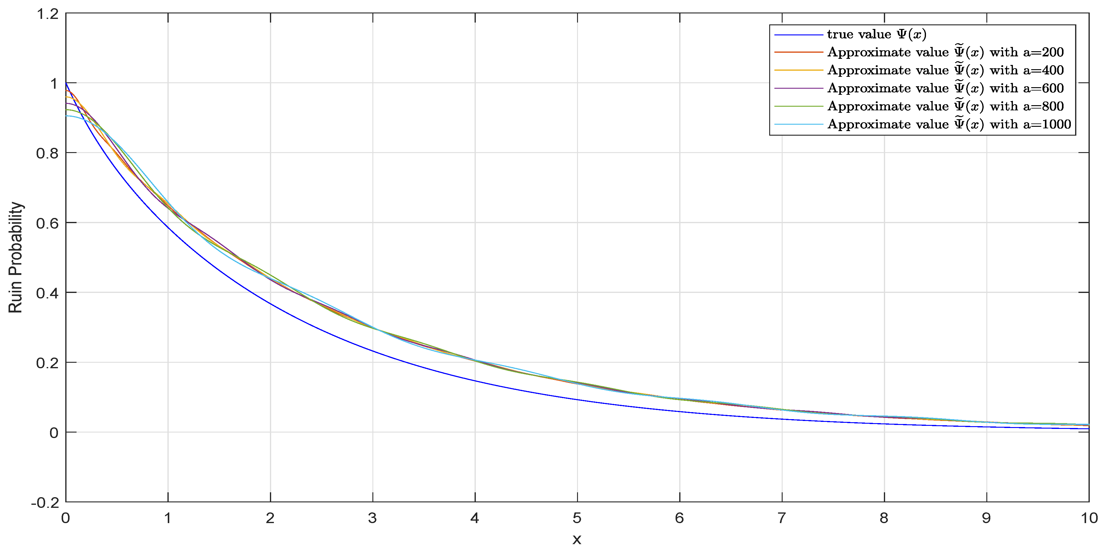
Firstly, according to Chau et al. [19] and Wang et al. [17], here we set the values of a as 200, 400, 600, 800, and 1000, respectively. In Figure 1, we plot the approximation $\tilde{\Psi }\left(x\right)$ with a = 200, 400, 600, 800, and 1000 and the parameter settings in Example 1, and then we list absolute error between the approximation $\tilde{\Psi }\left(x\right)$ and true value $\Psi \left(x\right)$ in different cases of a in Table 1.

Figure 1. The approximation $\tilde{\Psi }\left(x\right)$ with a = 200, 400, 600, 800, and 1000 and true value $\Psi \left(x\right)$.

Table 1. Absolute error between the approximation $\tilde{\Psi }\left(x\right)$ and $\Psi \left(x\right)$.

	Absolute Error
	x = 1	x = 2	x = 3	x = 4	x = 5	x = 6	Average Error
a = 200	0.0622	0.0706	0.0666	0.057	0.0451	0.035	0.056083
a = 400	0.0681	0.0726	0.0666	0.0586	0.0472	0.0354	0.058083
a = 600	0.0547	0.0689	0.0677	0.0599	0.049	0.0375	0.056283
a = 800	0.0571	0.0822	0.0649	0.0574	0.0504	0.034	0.057667
a = 1000	0.073	0.072	0.0686	0.0595	0.046	0.0382	0.05955

Next, from Table 1, by choosing the approximation value $\tilde{\Psi }\left(x\right)$ of $x=1,2,3,4,5,6$ points and comparing it with the real value, we can see that the average absolute error when $a=200$ is smaller than in other cases, so here we choose $a=200$ for subsequent simulation.

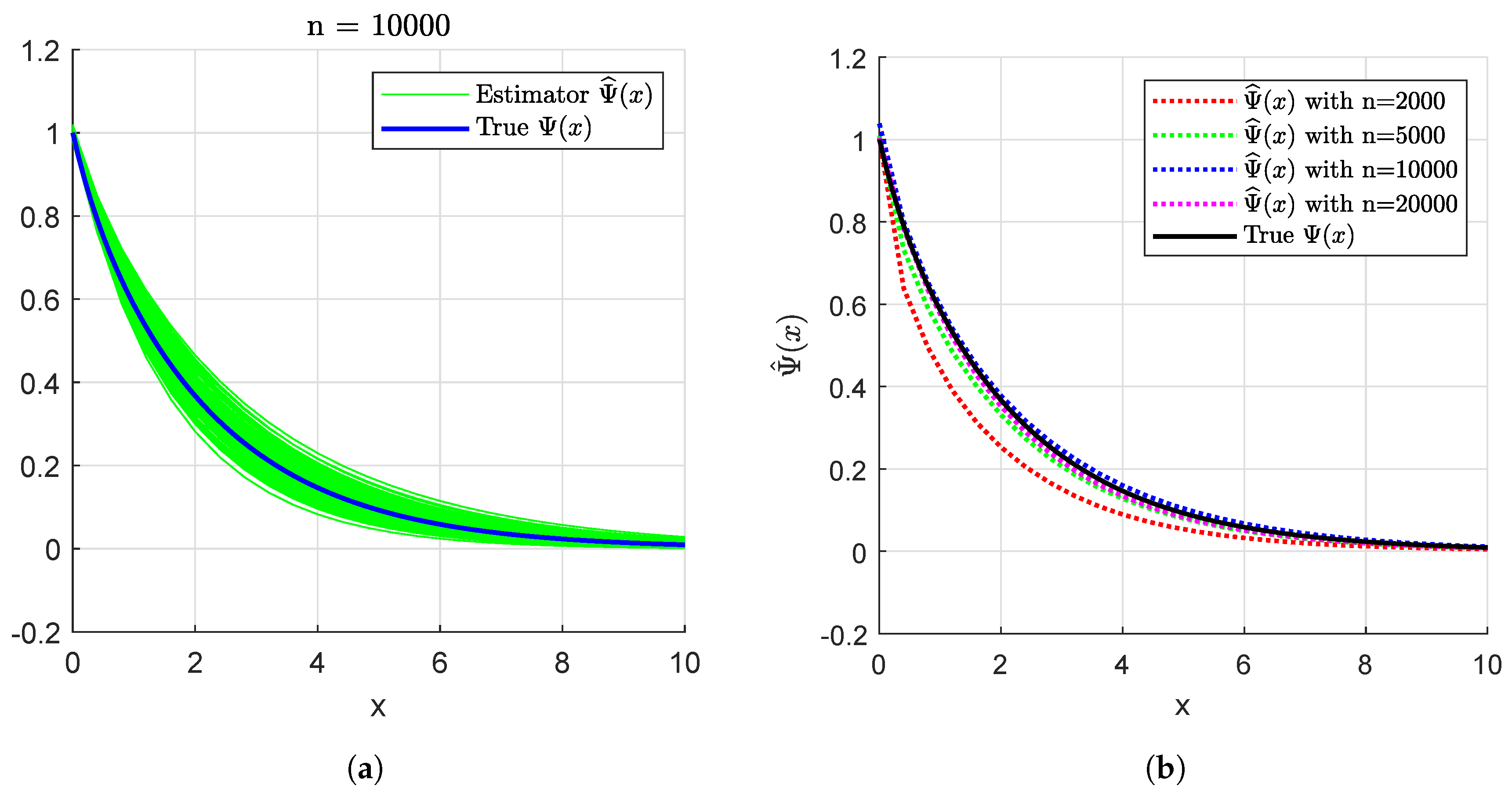
In Figure 2a, we plot the true ruin probability curve and 100 estimated curves with sample size n = 10,000 and the parameters setting in Example 1. In Figure 2b, we plot the true ruin probability curve and some mean curves with sample sizes n = 2000, 5000, 10,000, 20,000 and the parameter settings in Example 1, which are computed based on 100 simulation experiments.

Figure 2. (a) True curve (bold blue line) and 100 estimated curves (green lines) with sample size n = 10,000. (b) The estimator $\widehat{\Psi }\left(x\right)$ with sample sizes n = 2000, 5000, 10,000, 20,000.

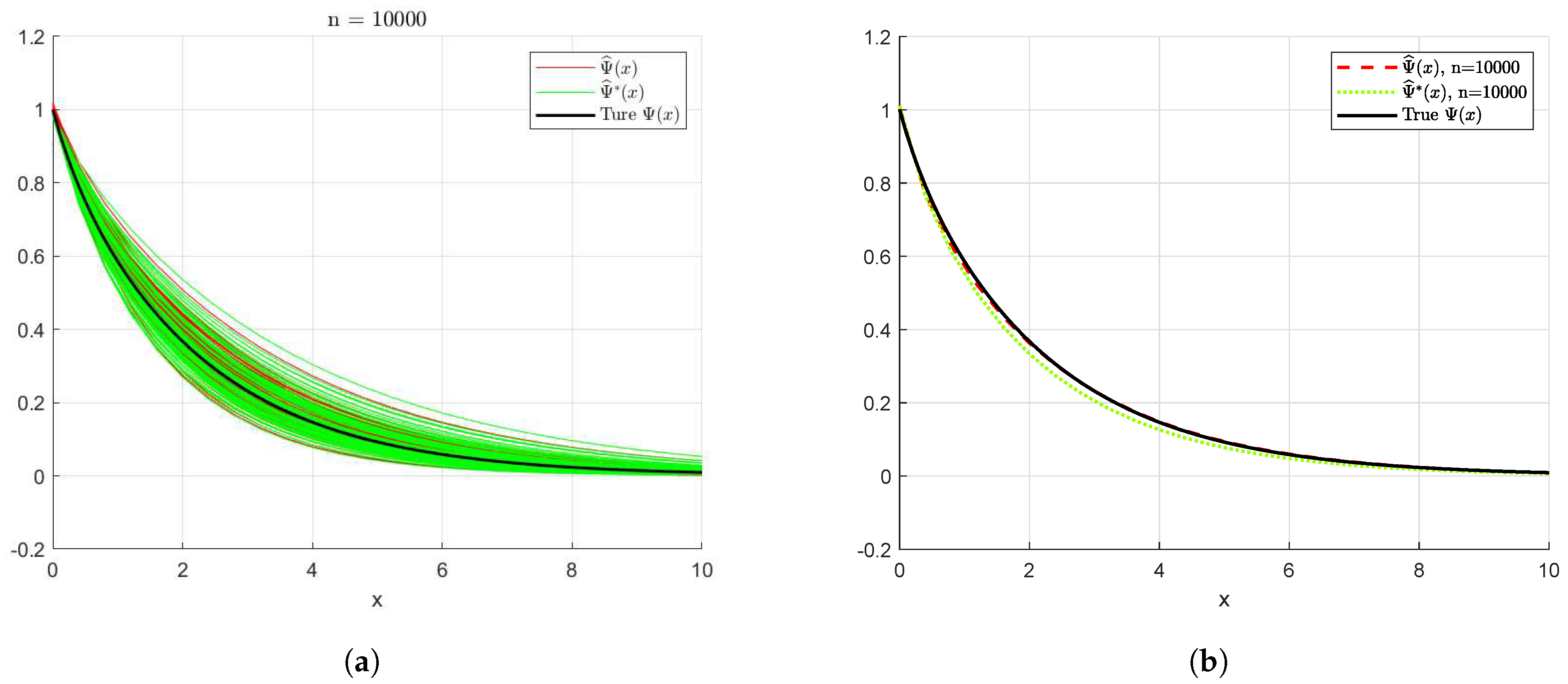
In Figure 3a, we plot 100 estimated curves, both with and without a threshold function, along with the true ruin probability curve. The sample size is set to n = 10,000, following the parameter settings in Example 1. In Figure 3b, We plot the mean estimators for a sample size of n = 10,000, both with and without a threshold function, as well as the true ruin probability curve, using the parameter settings from Example 1. These results are based on 100 simulation experiments.

Figure 3. (a) True curve (bold black line), 100 estimated curves without threshold function (green lines), and 100 estimated curves with a threshold function (red lines) with sample size n = 10,000. (b) The estimators mean of sample sizes n = 10,000 with and without a threshold function.

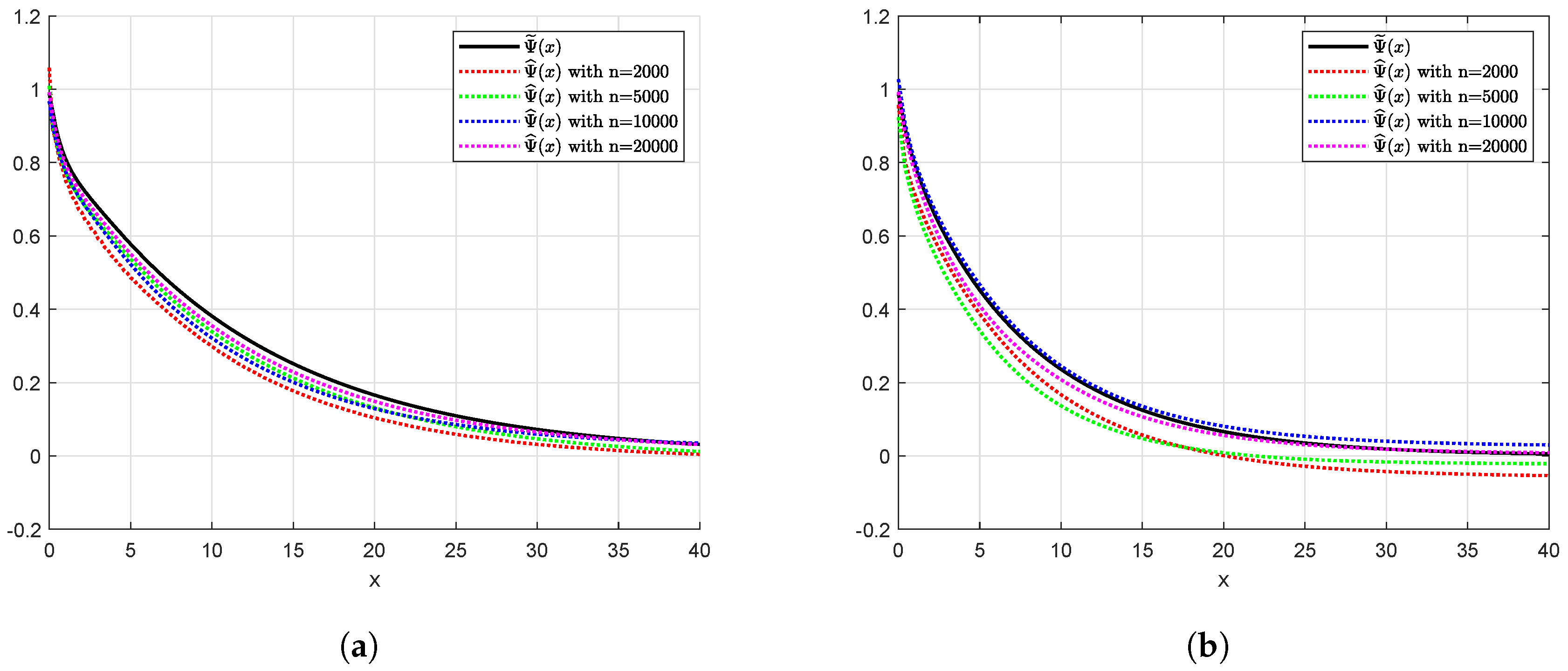
In Figure 4a, we present the mean curves for sample sizes n = 2000, 5000, 10,000, 20,000, along with the approximation $\tilde{\Psi }\left(x\right)$, using the parameter settings from Example 2. These results are based on 100 simulation experiments. Similarly, in Figure 4b, we display the mean curves for the same sample sizes, alongside the approximation $\tilde{\Psi }\left(x\right)$, using the parameter settings from Example 3, also derived from 100 simulation experiments.

Figure 4. (a) The estimator $\widehat{\Psi }\left(x\right)$ with sample sizes n = 2000, 5000, 10,000, 20,000 and the approximation $\tilde{\Psi }\left(x\right)$. (b) The estimator $\widehat{\Psi }\left(x\right)$ with sample sizes n = 2000, 5000, 10,000, 20,000 and the approximation $\tilde{\Psi }\left(x\right)$.

6. Conclusions

In this article, our result only discussed the asymptotic properties between the approximate ruin probability and its estimator but did not address the asymptotic relationship between the estimator of the ruin probability and its true value. This is because when using the Fourier-cosine method, the true value of the ruin probability can be closely approximated by selecting appropriate values for a and K. In our work, the values of a and K are based on Chau et al. [19], and we validated these choices in Figure 1 under the case where the jump sizes in the model follow an exponential distribution, confirming their appropriateness. For more information on choosing a and K, see references [16,17]. Additionally, we further verified the conclusion of Theorem 4.9 in Examples 2 and 3. In Examples 2 and 3, it is difficult to determine the true value of the ruin probability directly. However, it can be estimated using the Monte Carlo method with a large sample size. In theory, this estimate should be very accurate, though it requires significant computational time. Ideally, in Examples 2 and 3, we should compare the Monte Carlo estimates with the approximations from the Fourier-cosine method to further validate the appropriateness of the a and K values.

We apply the threshold estimation technique and the Fourier-cosine method to construct an estimator for the ruin probability in the Wiener–Poisson risk model, utilizing high–frequency data. The methodology in this paper can also estimate other ruin-related quantities, such as the Gerber–Shiu function. However, for the Gerber–Shiu function, additional parameters or functions must be estimated, making the analysis more complex.