1. Introduction
The inferential problem of drawing an inference about a common mean vector of several independent normal populations with unequal and unknown dispersion matrices is considered in this paper. We treat the problems of: (1) point estimation of ; (2) test for versus ; and (3) construction of confidence sets for .
Suppose there are
p-variate normal populations with common mean vector
and unknown covariance matrices
. Let
be independent
p-variate vector sample observations from the
i-th population (
) and
,
. For the
i-th population, let
be the sample mean vector and sample sum of squares and products matrix. Jointly,
provide minimal sufficient statistics for the unknown parameters
and
(
). It is well-known that one can use the familiar Hotelling’s
test for
and reject the null based on the
i-th dataset when
is large.
A confidence set for based on the i-th dataset is also readily obtained as
In
Section 2, we provide an unbiased estimate of
based on the minimal sufficient statistics and provide an expression for its estimated asymptotic variance. A test procedure for
and a confidence ellipsoid for
then readily follow. These results are asymptotic in nature.
An approximate procedure for a test set and a confidence set for
in our context was suggested by [
1] based on the notion of generalized
p-values [
2,
3,
4]. This is briefly mentioned in
Section 3. The authors clearly presented relevant algorithms to carry out the suggested procedures and also discussed their performance in terms of coverage probabilities and expected volumes in comparison with some existing methods. Notwithstanding their claim of anticipated better performance over existing procedures, the fact remains that the generalized
p-value-based procedure is indeed approximate and may not work well in some situations in view of the unknown and unequal nature of the population dispersion matrices (see Tables 5 and 6 in [
1]).
Exact tests for
and exact confidence sets for
can be derived by efficiently combining the
k independent Hotelling’s
statistics. Fortunately, several well-known exact procedures exist in the literature [
5,
6]. In
Section 4, we provide a review of these exact test procedures and in
Section 5, we provide a review of exact confidence sets. Local powers of the exact tests are discussed in
Section 6 based on a Taylor expansion of the power, and these are compared in
Section 7. In
Section 8, two applications are provided. First, we reproduce a dataset from [
5] for
,
, and
, each from
,
, and use it to construct a confidence set for the bivariate common mean vector based on the above exact procedures. Plots showing the confidence sets appear in
Figure 1. Our second example is based on data arising from Current Population Survey (CPS) conducted by the Bureau of the Census for the Bureau of Labor Statistics. It turns out that the sample sizes are large for the CPS data, thus enabling us to also include the large sample procedure described in
Section 2. Plots showing the confidence sets appear in
Figure 2,
Figure 3 and
Figure 4. For the sake of completeness, we have also plotted the confidence set derived from the generalized
p-value-based method [
1] in both the applications. We conclude the paper with some conclusions in
Section 9.
2. A Large Sample Procedure
In this section, we propose an unbiased estimate of
, which is essentially a generalization of the familiar Graybill–Deal estimate [
7] of
in the case of univariate normal populations. This estimate and its estimated asymptotic variance in the univariate case are given by:
A test for versus is based on the standard normal Z statistic defined as . An asymptotic confidence interval for is given by .
As a generalization to the multivariate case, we propose:
An asymptotic test for
versus
can then be based on the
statistic:
The
asymptotic ellipsoidal confidence set for
is provided by:
Our simulation studies (see
Appendix A) demonstrate the robustness of the
cut-off point for variations in the unknown dispersion matrices. Applications of (
5) for a real ASEC dataset appear in
Section 8.
3. Confidence Set Based on Generalized p-Value
Tsui and Weerahandi, 1989 [
2] came up with a novel idea to deal with uncommon inference problems. Examples include the ANOVA problem under variance heteroscedasticity, the test for treatment of variance components in a one-way random effects model, the test for reliability parameter
when
, independent of
, and so on. The method is based on a function
of underlying random variable
X, its observed value
x, and the parameter of interest
, with
being a nuisance parameter. Under certain conditions of
, a test for
and a confidence set for
can be derived. Their method is referred to as the generalized
p-value-based approach.
In our context, following [
1], Ref. [
2] suggested the following algorithm to construct a confidence ellipsoid for
. An extension of the generalized
p-value method from a common univariate normal mean with unknown variances to the case of a common mean vector with unknown dispersion matrices is highly nontrivial, and the authors deserve a lot of credit for providing a solution. Starting with the basic ingredients, namely,
, define
,
,
, and
.
For :
Generate from .
Generate independent and from , .
Compute and .
Compute .
(End j loop)
Compute , , and , where , .
Let
be the
-th percentile of
,
; then, the confidence ellipsoid of
can be obtained from the inequality
4. Exact Tests for versus
To develop the exact test for testing versus based on all the datasets, we proceed as follows. Recall that satisfies , where follows an F-distribution with and degrees of freedom. Our test procedure rejects when , with being the Type I error level and being the observed value of F under . A test for based on a p-value, on the other hand, is based on , and we reject at the level if . It is easy to check that the two approaches are obviously equivalent.
A random p-value which follows a uniform distribution under the null hypothesis is defined as , where . All suggested exact tests for are based on and values, and their properties, including size and power, are studied under and . To simplify notations, we denote by small p and by large P. Four exact tests based on p values and one exact test based on , as available in the literature, are listed below.
4.1. Tippett’s Test
This minimum
p-value test was proposed by [
8], who noted that, if
are independent
p-values from continuous test statistics, then each has a uniform distribution under
. According to this method, the null hypothesis
is rejected at the
level of significance if
, where
. Incidentally, this test is equivalent to the test based on
as suggested by [
9].
4.2. Wilkinson’s Test
This test statistic proposed by [
10] is a generalization of Tippett’s test that uses the
r-th smallest
p-value (
) as a test statistic. The null hypothesis
will be rejected if
, where
follows a
Beta distribution with parameters
r and
under
and where
satisfies
. Obviously, this procedure generates a sequence of tests for different values of
, and an attempt has been made to identify the best choice of
r.
4.3. Inverse Normal Test
This exact test procedure, which involves transforming each
p-value to the corresponding normal score, was proposed independently by [
11,
12]. Using this inverse normal method, the null hypothesis
will be rejected at the
level of significance if
, where
denotes the inverse of the cumulative distribution function (CDF) of a standard normal distribution, and
stands for the upper
-level cut-off point of a standard normal distribution.
4.4. Fisher’s Inverse -Test
This inverse
-test is one of the most widely used exact test procedures for combining
k independent
p-values [
13]. This procedure uses the
to combine the
k independent
p-values. Then, using the connection between uniform and
distributions, the null hypothesis
is rejected if
, where
denotes the upper
critical value of a
-distribution with
degrees of freedom.
4.5. Jordan–Kris Test
Jordan and Krishnamoorthy, 1995 [
5] considered a weighted linear combination of Hotelling’s
statistic, namely
, where
, and
with
. The null hypothesis
will be rejected if
, where
. In applications,
a is computed by using the approximation
, where
,
,
, and
.
5. Exact Confidence Sets for the Mean Vector
In this section, we present some exact confidence sets for
, essentially based upon inverting the acceptance sets resulting from the discussion in
Section 4.
5.1. Confidence Set Based on Jordan–Kris Method
Following the method proposed in [
5], which is presented in
Section 4.5, a
confidence ellipsoid for
is a set of values
satisfying the following inequality:
where
,
, and
.
5.2. p-Value-Based Confidence Sets
All the p-value-based confidence sets are obtained by inverting the corresponding acceptance sets; the following are the results. We define .
5.2.1. Confidence Set Based on Tippett’s Method
A Tippett’s confidence set for is a set of values satisfying .
5.2.2. Confidence Set Based on Wilkinson’s Method
A Wilkinson’s (order r) confidence set for is a set of values satisfying .
5.2.3. Confidence Set Based on the INN Method
A confidence set for based on inverse normal (INN) method is a set of values satisfying .
5.2.4. Confidence Set Based on Fisher’s Method
A
confidence set for
based on Fisher’s inverse
-test is a set of values
satisfying
.
Remark 1. Unlike the large sample-based confidence ellipsoid presented in Section 2, the generalized p-value-based confidence ellipsoid presented in Section 3, and the Jordan–Kris confidence ellipsoid presented in Section 4, the p-value-based confidence sets described above may not always lead to confidence ellipsoids! 6. Expressions of Local Powers of Proposed Exact Tests
In this section, we provide the expressions of local powers of the suggested exact tests. A common premise is that we derive an expression of the power of a test under , carry out its Taylor expansion around , where , and retain terms of order .
The probability density functions (PDFs) of the
F statistic under the null and alternative hypotheses that will be required in the sequel are given below. Below,
stands for the non-centrality parameter when
is chosen as an alternative value.
The final expressions of the local powers of the proposed tests are given below in the general case and also in the special case when
. For detailed proofs of all technical results, we refer to
Appendix B of this paper.
6.1. Local Power of Tippett’s Test
where
.
6.2. Local Power of Wilkinson’s Test
where
is equivalent to
, with
.
Remark 2. For the special case , , as expected, because , implying .
6.3. Local Power of Inverse Normal Test
where
,
,
,
,
is standard normal PDF, and
is standard normal CDF.
6.4. Local Power of Fisher’s Test
where
;
;
exp[2];
gamma[1,
k];
;
;
.
6.5. Local Power of Jordan–Kris Test
where
stands for expectation with respect to
under
.
7. Comparison of Local Powers
It is interesting to observe from the above expressions that, in the special case of equal sample size, local powers can be readily compared, irrespective of the values of the unknown dispersion matrices , .
Table 1 represents values of the second term of local power in the case of equal sample size
n given above in (
11)–(
15), apart from the common term
, for different values of
k,
p, and
n. A comparison of the second term of local power of Wilkinson’s test for different values of
r is provided in
Table 2 for
,
, and
. Throughout, we have used
. It turns out that the exact tests based on the inverse normal and Jordan–Kris methods perform the best. It also appears from
Table 2 that an optimal choice of
r for Wilkinson’s method is nearly
.
8. Applications
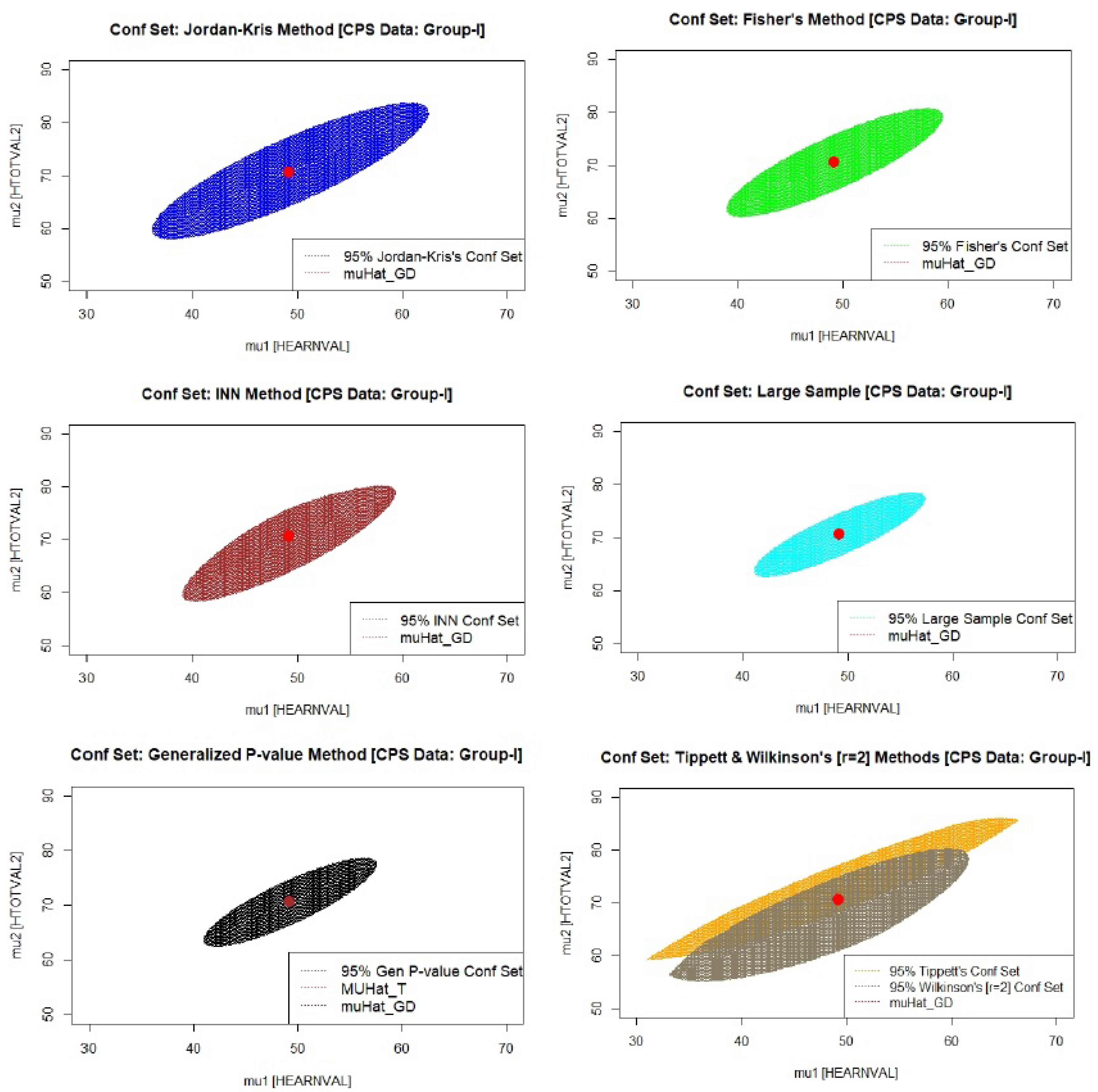
8.1. Confidence Set Comparison Using Simulated Data
In this section, we follow the framework in [
5], who simulated bivariate samples of 12 vectors (equal sample size
) each from two bivariate normal distributions,
and
, with
,
, and
. Summary statistics based on these two simulated datasets are:
,
,
,
, and
.
Based on the above simulated data, we present below the 95% confidence sets for
resulting from the five exact methods (
Figure 1) and the method based on the generalized
p-value. It turns out that the INN method followed by the Jordan–Kris and Fisher methods yield smaller observed confidence sets than the Tippett and Wilkinson (
) methods. As remarked earlier, although the confidence ellipsoid based on the generalized
p-value method seems to have a smaller volume, its coverage probability cannot be guaranteed.
Simulated Coverage Probabilities
In this section, we present the simulated coverage probabilities (CPs) for various confidence sets discussed in
Section 3 and
Section 5. These CPs have been estimated through simulation studies based on a bivariate normal distribution, with parameters outlined in
Section 8.1.
Table 3 provides the 95% CP values for an equal sample size case in the six methods, including the generalized
p-value method. As expected, the CP increases with the sample size, indicating improved reliability of the confidence sets as the sample size increases.
To evaluate the robustness of these methods under distributional misspecification, we performed a simulation study using a multivariate Laplace distribution, applying the same parameters as described previously. We calculated the 95% coverage probabilities for the six confidence sets. The results, presented in
Table 4, demonstrate that most methods remain robust despite the distributional misspecification. However, Wilkinson’s method exhibits a decline in coverage probabilities as the sample size increases, indicating some sensitivity to the underlying distribution. In general, these methods generally maintain their reliability even when the assumed distribution differs from the true one.
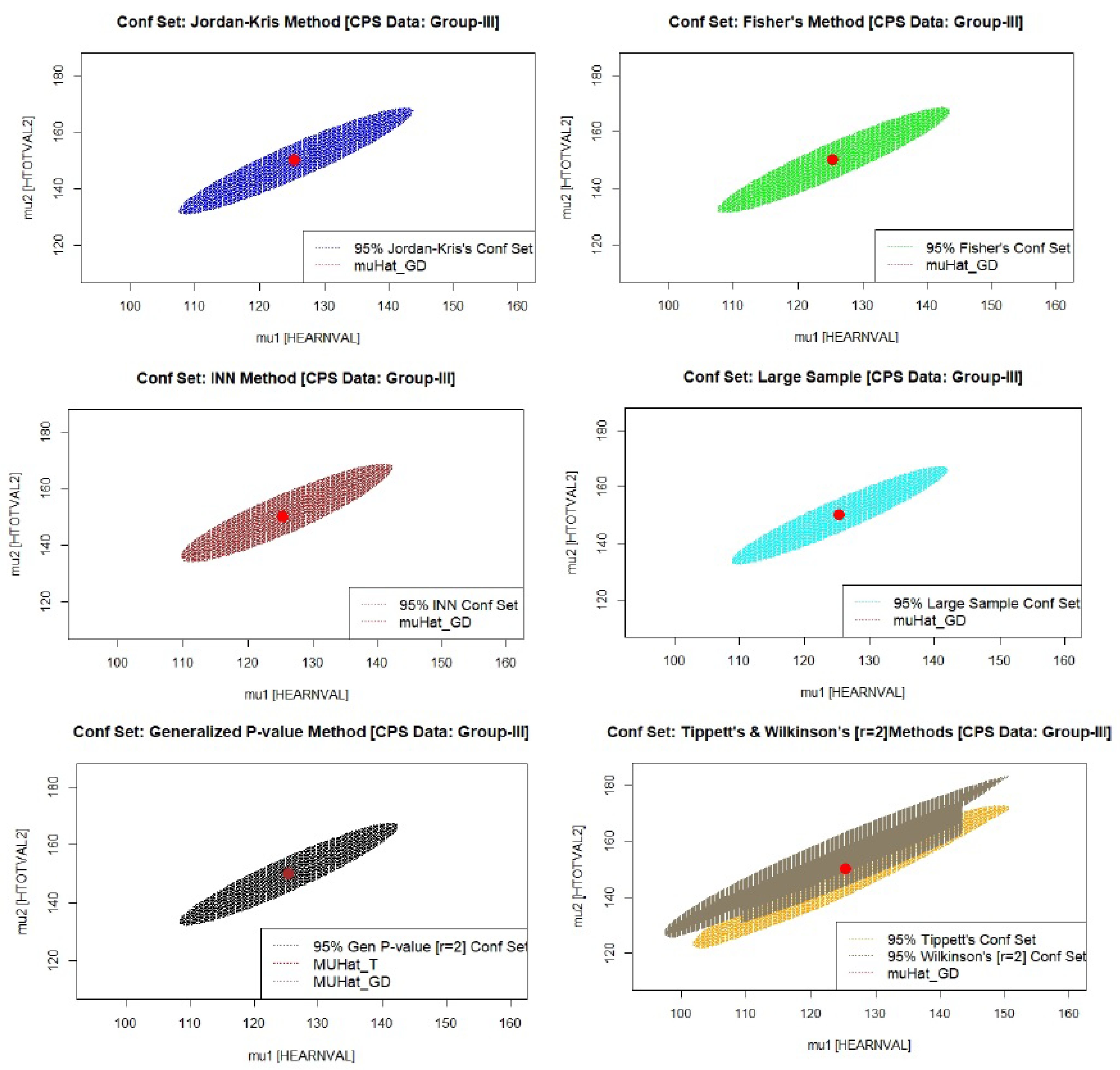
8.2. Data Analysis: Current Population Survey (CPS) Annual Social and Economic (ASEC) Supplement
In this section, we provide a statistical analysis of data arising from the Current Population Survey (CPS) Annual Social and Economic (ASEC) Supplement 2021, conducted by the Bureau of the Census for the Bureau of Labor Statistics.
Under CPS, typically some 70,000 housing units or other living quarters are assigned for interview each month; about 50,000 of them that contain approximately 100,000 persons 15 years old and over are interviewed. The universe in this survey is the civilian non-institutional population of the United States living in housing units and members of the armed forces living off post or living with their families on post. Sampling units are scientifically selected (based on a probability sample) on the basis of area of residence to represent the nation as a whole, individual states, and other specified areas.
Although the main purpose of the survey is to collect information on the employment situation, a very important secondary purpose is to collect information on the demographic status of the population, such as age, sex, race, marital status, educational attainment, and family structure. The statistics resulting from these questions serve to update similar information collected once every 10 years through the decennial census and are used by government policymakers and legislators as important indicators of our nation’s economic situation and for planning and evaluating many government programs. CPS is the only source of monthly estimates of total employment (both farm and non-farm); non-farm self-employed persons, domestics, and unpaid workers in non-farm family enterprises; wage and salary employees; and, finally, estimates of total unemployment.
The Annual Social and Economic (ASEC) Supplement contains the basic monthly demographic and labor force data described above, plus additional data on work experience, income, non-cash benefits, health insurance coverage, and migration. Since 1976, the survey has been supplemented with about 6000 Hispanic households from which at least 4500 are interviewed. However, in 2002, another sample expansion occurred to help improve states’ estimates of the Children’s Health Insurance Program (CHIP), resulting in the addition of 19,000 households, which raised the total sample size for the ASEC to about 95,000 households. All current population reports are available online at
https://www.census.gov/library/publications.html (accessed on 19 November 2022).
For the purpose of our data analysis, we mainly consider two variables out of a wide range of available data: total income and income components covering nine non-cash income sources: food stamps, school lunch program, employer-provided group health insurance plan, employer-provided pension plan, personal health insurance, Medicaid, Medicare, or military health care, and energy assistance. Characteristics such as age, sex, race, household relationship, and Hispanic origin are shown for each person in the enumerated household. Although the above type of data is available for all 50 U.S. states, we focus on the data from California (CA), as it is argued that this data source is the most reliable, and the sample sizes are fairly large. There are 58 counties in CA, and the table below shows a summary of the bivariate sample mean vectors and 2 × 2 sample variance–covariance matrices for 13 selected counties in CA, divided into three groups (
Table 5). We observe that the simple mean vectors in each group are fairly close, suggesting a common population mean vector within the chosen counties of a group. The 95% confidence sets of the common mean vector based on the methods discussed in this paper appear in
Figure 2,
Figure 3 and
Figure 4. The location of the well-known Graybill–Deal estimate of the common mean vector is shown in each ellipsoid. As an illustration, we have also added a figure (
Figure 5) depicting three confidence sets under the Fisher method for the three groups for the sake of comparison.
9. Conclusions
This paper presents a comprehensive approach to drawing inferences about a common mean vector from several independent multi-normal populations with unequal and unknown dispersion matrices. By developing both asymptotic and exact methods, we offer robust tools for statistical analysis that can be applied to a variety of practical situations, including statistical meta-analysis. The procedures based on the standardized Graybill–Deal estimate of the common mean vector prove to be effective and easy to implement for large sample sizes. In small samples, however, several exact procedures with good frequentist properties exist.
A notable limitation of our approach is its reliance on the assumption of multivariate normality, which may not be applicable in all practical settings. Although our simulations under distributional misspecification, such as using a multivariate Laplace distribution, indicate robustness, this robustness could be sensitive to more extreme deviations from normality or in the presence of heavy tails. Future research could explore the extension of these methods to broader classes of distributions, enhancing their applicability in real-world data analysis. We anticipate that the methods discussed will find practical use and inspire further developments in the field of multivariate analysis.
Author Contributions
Conceptualization, B.K.S. and Y.G.K.; methodology, B.K.S. and Y.G.K.; software, Y.G.K. and A.M.M.; validation, B.K.S., Y.G.K. and A.M.M.; formal analysis, A.M.M., B.K.S. and Y.G.K.; writing—original draft preparation, B.K.S., A.M.M. and Y.G.K.; writing—review and editing, B.K.S., A.M.M. and Y.G.K.; visualization, Y.G.K.; supervision, B.K.S. and Y.G.K. All authors have read and agreed to the published version of the manuscript.
Funding
This research received no external funding.
Data Availability Statement
The original contributions presented in the study are included in the article, further inquiries can be directed to the corresponding author.
Acknowledgments
The authors are thankful to Tommy Wright for his encouragement and Thomas Mathew for his helpful comments. The first author thankfully acknowledges the summer research support from the University of Maryland Baltimore County (UMBC) Summer Research Faculty Fellowship (SURFF) program. Our heartfelt thanks go to three reviewers for their excellent comments, which helped us clarify several key points and enhance the quality of this paper.
Conflicts of Interest
The three authors declare no conflicts of interest.
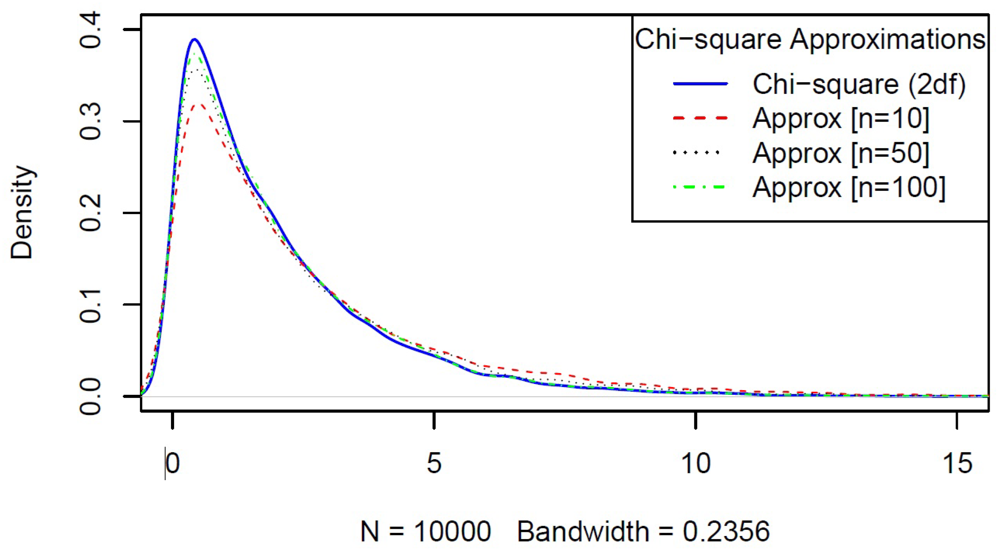
Appendix A. Robustness of the χ2 Cut-Off Point
We present here the results of our simulation based on
replications related to the cut-off point of the test statistic given by Equation (
4). We have taken several scenarios of dispersion matrices and
. Our simulation studies demonstrate the robustness of the
cut-off point for variations in the unknown dispersion matrices (see
Table A1 and
Figure A1). As shown in
Figure A1, the approximation remains good even with a smaller sample size of
.
Table A1.
95% Cut-off points for different sample sizes and dispersion matrices.
Table A1.
95% Cut-off points for different sample sizes and dispersion matrices.
| Dispersion Matrices | 95% Cut-Off Points |
|---|
| n = 50 | n = 100 |
|---|
|
|
| 6.63 | 6.29 |
|
|
| 6.64 | 6.21 |
|
|
| 6.62 | 6.24 |
|
|
| 6.62 | 6.24 |
|
|
| 6.62 | 6.26 |
Figure A1.
Chi-square with 2 degrees of freedom and large sample distributions with , , and .
Figure A1.
Chi-square with 2 degrees of freedom and large sample distributions with , , and .
Appendix B. Proofs of Local Powers of Exact Tests
We begin by stating a result that will be crucial for providing the main results on local power of all
p-value-based exact tests. We denote
to represent the CDF of a central
F-distribution with
and
degrees of freedom.
Lemma A1. Let T be a random variable with PDF and CDF , . Definewhere follows an F distribution with and degrees of freedom , and satisfiesThen, Proof. Obviously,
From Equation (
A2), by differentiating both sides with respect to
t, we obtain:
which implies that
Lemma A1 (which is Equation (
A3)) follows upon combining Equations (
A4) and (
A6). □
Appendix B.1. Local Power of Tippett’s Test [LP(T)]
Recall that Tippett’s exact test rejects the null hypothesis if
, where
. This leads to:
By applying the approximate distribution of
under the alternative hypothesis following its Taylor expansion around
, the local power of Tippett’s test is calculated as follows:
For the special case
and
, the local power of Tippett’s test reduces to:
Appendix B.2. Local Power of Wilkinson’s Test [LP(W r)]
Using the
r-th smallest
p-value
as a test statistic, the null hypothesis will be rejected if
, where
∼
Beta under
, and
satisfies:
This leads to:
where
is a permutation of
. Applying Lemma A1, we obtain:
Let us now apply the following fact in (
A10):
Permuting
over
, we obtain, for any fixed
l:
The second term above follows upon noting that, when is permuted over , each term appears exactly times for each . The third term, likewise, follows upon noting that, when is permuted over , each term appears exactly times for each .
Adding the above three terms and applying (
A9), we obtain:
For the special case
, and
, the local power of Wilkinson’s test reduces to:
Appendix B.3. Local Power of Inverse Normal Test [LP(INN)]
Under this test, the null hypothesis will be rejected if
, where
,
is the inverse CDF, and
is the upper
level critical value of a standard normal distribution. This leads to:
First, let us determine the PDF of
U under
,
, via its CDF
:
This implies:
Let us define
,
, and
as
,
, and
. Using these three quantities, we now approximate the distribution of
U as:
Using the above result, the local power of the inverse normal test is obtained by approximating its power, which is
, as:
Substituting back the expressions for
and
results in:
For the special case
, the local power of the Inverse Normal (INN) test reduces to:
Appendix B.4. Local Power of Fisher’s Test [LP(F)]
According to Fisher’s exact test, the null hypothesis will be rejected if
, where
, and
is the upper
-level critical value of a
-distribution with
degrees of freedom. This leads to:
In a similar manner as the inverse normal test in
Appendix B.3, first let us determine the PDF of
V under
,
, via its CDF
:
This implies:
The expectation of V can now be obtained as:
Let us approximate the distribution of
V under the alternative using the method of moments, which implies
, and hence,
. We can now approximate the distribution of
V under
as:
Here,
stands for a Gamma random variable with scale parameter
and shape parameter
, with the PDF
. By the additive property of independent
corresponding to
, we readily obtain the approximate distribution of
as:
The local power of Fisher’s test under
is then obtained as follows:
We now expand
around
to obtain:
Here, we have used the fact that: (1)
; (2)
; and (3)
, where
is a constant. Therefore, in our context,
. Now, substituting back the expressions for
A in (A18) results in:
For the special case
and
, the local power of Fisher’s test reduces to:
Appendix B.5. Local Power of the Jordan–Kris Test [LP(JK)]
According to this test based on a weighted linear combination of Hotelling’s
, the null hypothesis
will be rejected if
, where
,
, and
. In applications,
a is computed by using the approximation
, where
,
,
, and
.
Note that
and its local expansion around
are given by:
Using the above first-order expansion of
leads to the following local power of
T:
where
stands for expectation with respect to
under
.
For the special case
, the local power of this test based on a weighted linear combination of Hotelling’s
reduces to:
References
- Lin, S.; Lee, J.C.; Wang, R. Generalized inferences on the common mean vector of several multivariate normal populations. J. Stat. Plan. Inference 2007, 137, 2240–2249. [Google Scholar] [CrossRef]
- Tsui, K.W.; Weerahandi, S. Generalized p-values in significance testing of hypotheses in the presence of nuisance parameters. J. Am. Stat. Assoc. 1989, 84, 602–607. [Google Scholar] [CrossRef]
- Weerahandi, S. Generalized Confidence Intervals. J. Am. Stat. Assoc. 1993, 88, 899–905. [Google Scholar] [CrossRef]
- Weerahandi, S. Exact Statistical Methods for Data Analysis; Springer Science & Business Media: Berlin/Heidelberg, Germany, 2003. [Google Scholar]
- Jordan, S.M.; Krishnamoorthy, K. Confidence regions for the common mean vector of several multivariate normal populations. Can. J. Stat. 1995, 23, 283–297. [Google Scholar] [CrossRef]
- Kifle, Y.G.; Moluh, A.M.; Sinha, B.K. Comparison of Local Powers of Some Exact Tests for a Common Normal Mean with Unequal Variances. In Methodology and Applications of Statistics; Springer: Berlin/Heidelberg, Germany, 2021; pp. 77–101. [Google Scholar]
- Graybill, F.A.; Deal, R. Combining unbiased estimators. Biometrics 1959, 15, 543–550. [Google Scholar] [CrossRef]
- Tippett, L.H.C. The Methods of Statistics. J. R. Stat. Soc. Ser. Stat. Soc. 1932, 95, 323–325. [Google Scholar]
- Cohen, A.; Sackrowitz, H. Testing hypotheses about the common mean of normal distributions. J. Stat. Plan. Inference 1984, 9, 207–227. [Google Scholar] [CrossRef]
- Wilkinson, B. A statistical consideration in psychological research. Psychol. Bull. 1951, 48, 156. [Google Scholar] [CrossRef] [PubMed]
- Stouffer, S.A.; Suchman, E.A.; DeVinney, L.C.; Star, S.A.; Williams, R.M., Jr. The American Soldier: Adjustment during Army Life; Princeton University Press: Princeton, NJ, USA, 1949; Volume 1. [Google Scholar]
- Lipták, T. On the combination of independent tests. Magyar Tud. Akad. Mat. Kutato Int. Kozl. 1958, 3, 171–197. [Google Scholar]
- Fisher, R. Statistical Methods for Research Workers, 4th ed.; Oliver and Boyd: Edinburgh, UK; London, UK, 1932. [Google Scholar]
| Disclaimer/Publisher’s Note: The statements, opinions and data contained in all publications are solely those of the individual author(s) and contributor(s) and not of MDPI and/or the editor(s). MDPI and/or the editor(s) disclaim responsibility for any injury to people or property resulting from any ideas, methods, instructions or products referred to in the content. |
© 2024 by the authors. Licensee MDPI, Basel, Switzerland. This article is an open access article distributed under the terms and conditions of the Creative Commons Attribution (CC BY) license (https://creativecommons.org/licenses/by/4.0/).


