Real-Data-Based Study on Divorce Dynamics and Elimination Strategies Using Nonlinear Differential Equations

Abstract

This paper presents a novel approach to studying divorce dynamics and elimination strategies using nonlinear differential equations. A mathematical model is formulated to capture the key factors influencing divorce rates. The model undergoes a rigorous theoretical analysis, including parameter estimation, solution existence/uniqueness, positivity, boundedness, and invariant regions. A qualitative analysis explores equilibria, stability conditions, and a sensitivity analysis. Numerical simulations and discussions are presented to validate the model and shed light on divorce dynamics. Finally, conclusions and future research directions are outlined. This work offers valuable insights for understanding and potentially mitigating divorce rates through targeted interventions.

1. Introduction

Divorce, characterized as the formal termination of marriage, represents a significant socio–legal phenomenon that has garnered considerable scholarly attention across diverse academic fields. Initially analyzed within the realms of law and ethics, the focus has shifted towards understanding its psychological and social ramifications. Studies suggest that the precipitants of divorce are complex and multifarious, encompassing issues like failures in communication, economic duress, unfaithfulness, and shifts in personal values or life objectives. Amato and Previti (2003) in [1] posit that individual dissatisfaction and relational dynamics are pivotal in the disintegration of marital unions, underlining the nuanced interconnection between personal discontent and couple interactions. As cultural perceptions evolve, the stigma around divorce waxes and wanes, mirroring broader societal shifts in views on marriage, gender roles, and personal independence.

Variations in divorce rates are evident across different regions and are shaped by socio–economic, cultural, and legal influences. For instance, in the United States, there has been a notable trend towards the stabilization or reduction of divorce rates in recent years, which has been partially attributed to older ages at first marriage and greater societal acceptance of pre-marital cohabitation (Copen, Daniels, Vespa, Mosher, 2012 in [2]). On the global stage, the divorce prevalence differs markedly, influenced by local cultural prohibitions and economic limitations. Ongoing research endeavors to elucidate the enduring impacts of divorce, especially on children, revealing diverse consequences for emotional well-being, educational achievement, and subsequent relationship stability. The dynamic and evolving nature of divorce, characterized by both its origins and repercussions, continues to be a focal point of scholarly inquiry, emphasizing the complex interrelation between individual choices and societal frameworks.

The ramifications of divorce permeate well beyond the immediate emotional and legal dissolution of a marriage, profoundly affecting all involved parties, including the spouses and their children. For the partners, the repercussions are complex and multi-dimensional, touching emotional, financial, and social aspects of life. Research frequently underscores the emotional distress faced by individuals undergoing divorce, manifesting as loss, anger, depression, and anxiety. For example, in [3], Amato (2000) observed that individuals who have undergone divorce tend to report lower well-being levels compared to those who remain married, with these adverse effects often persisting years after the divorce has been finalized. Financially, the division of assets, coupled with potential decreases in income and increases in living expenses, can lead to economic instability. This issue disproportionately affects women, particularly those who may have been out of the workforce for extended periods. Socially, divorce often necessitates the reorganization of friendships and family relations, compelling the formation of new social networks. Children, though not direct participants in the divorce proceedings, encounter a distinct set of challenges with potential long-term consequences. Research indicates that children from divorced families are prone to educational disruptions, behavioral issues, and a heightened risk of mental health problems. Kelly and Emery (2003) in their landmark longitudinal study [4] noted that although most children adjust over time, they initially experience significant negative impacts, including distress, anger, and disbelief.

On a broader scale, the societal implications of divorce are considerable, influencing community structures and norms. Fluctuating divorce rates can affect community stability, alter familial configurations, and modify societal views on marriage and family life. Economically, an increase in divorce rates may intensify demands on social service systems and housing needs. Culturally, as societies contend with rising divorce occurrences, there may be changes in the stigma associated with divorce, variations in marriage and cohabitation trends, and evolution in legal norms related to family rights and responsibilities. Therefore, the extensive effects of divorce at both the micro and macro levels are significant, necessitating continued research to enhance its understanding and address its impacts.

Ordinary differential equations (ODEs) are essential in epidemiology because they provide a structure for simulating the movement of infectious illnesses within populations [5,6,7]. Mathematical models like the SIR model categorize the population into distinct compartments, including susceptible, infected, and recovered individuals. These models employ ODEs to depict the movement of individuals between these compartments over time, taking into account parameters like transmission rates and recovery rates. Through solving these equations, scientists are able to forecast the propagation of diseases, gauge the effectiveness of measures like vaccination and social distancing, and evaluate the contributing causes of outbreaks. ODE-based models are crucial tools for public health officials to strategize and execute successful disease control and prevention measures.

We employ mathematical epidemiology, particularly, models based on ODEs, to simulate divorce because it effectively analyzes dynamic systems, similar to how infectious diseases propagate. Using ODEs, which let us figure out important factors that affect things, look at complex relationships, and predict future patterns, we can accurately describe how quickly divorce spreads through social networks. These models offer a versatile framework for integrating many societal and individual elements, providing insights into the mechanisms that cause divorce. Furthermore, ODE-based models are valuable in formulating social policies and interventions because they can pinpoint key areas where even minor adjustments can have a significant effect on divorce rates. This makes ODE-based models a reliable instrument for comprehending and tackling the complexities of divorce dynamics.

Mathematical models of divorce are essential for comprehending the intricate dynamics that impact the stability and termination of marriages. By utilizing these models, researchers and policymakers may forecast divorce rates, discern underlying causes that contribute to marital breakdowns, and assess the efficacy of measures aimed at enhancing marriages. Comprehending this is crucial not just for scholarly investigation but also for developing strategies that could mitigate the societal and individual expenses linked to divorce. An efficient method for statistically modeling divorce is by using ODEs. These equations can mathematically represent the rate at which the condition of a marital relationship changes over time. Researchers can simulate alternative scenarios and results by establishing differential equations that mirror different features of marital interactions. For example, the model can include variables that indicate positive interactions, such as communication and shared interests, as well as negative interactions like disagreements and discontent. To assess the stability of a marital relationship, one might examine the equilibrium points of the system, where the rates of positive and negative interactions are in balance. Gottman and Murray [8], researchers in the field, employed this method to forecast marital dissolution by creating a system of ODEs using longitudinal couple data. Their findings indicated that the model was able to accurately predict divorce with considerable precision.

The theoretical basis for employing ODEs in divorce modeling often entails formulating a hypothesis regarding the factors that contribute to divorce and subsequently converting these variables into mathematical expressions. For example, factors such as love, satisfaction, and conflict can be depicted as functions that dynamically evolve over time based on their mutual influences. The parameters of the model can be obtained from empirical data, which are usually collected through surveys or longitudinal studies and are subsequently utilized to solve the differential equations. The answers to these equations facilitate comprehension of how alterations in one dimension of the connection impact the other variables. An examination of the model through theoretical research, including stability analysis and bifurcation theory, aids in the identification of crucial thresholds at which a marriage may transition from a stable to an unstable state, potentially resulting in separation or divorce. This modeling technique not only helps us understand the changes and processes involved in marriage breakdown, but it also gives a quantitative method for assessing the effectiveness of interventions aimed at enhancing marital stability [9]. Mathematical models, especially when they are validated and improved with real-world data, provide a strong perspective for analyzing and comprehending the dynamics of marital relationships. They offer both theoretical insights and practical applications in the fields of family psychology and social policy.

This manuscript is structured as follows: In Section 2, the construction of the divorce model is elucidated. Section 3 offers a comprehensive qualitative analysis of the model, addressing the estimation of parameters, the conditions for the existence and uniqueness of solutions, the identification of an invariant region, and the evaluation of solutions for positivity and boundedness. The stability of the divorce model is scrutinized in Section 4, where both local and global properties of the equilibria are explored. An investigation into how various parameters influence the basic reproduction number (${\mathcal{R}}_0$) is conducted in Section 5. Section 6 details the evaluation of the model’s epidemiological compartments through extensive numerical simulations. The manuscript concludes in Section 7 with a synthesis of the principal findings and a delineation of prospective directions for further research.

2. Model Formulation

This section is designed for the development of a mathematical model for divorce transmission. The total population is divided into five compartments. The five compartments are Susceptible $S\left(t\right)$, Married $M\left(t\right)$, Short Breakup $E\left(t\right)$, Long Breakup $F\left(t\right)$, and Divorced $D\left(t\right)$. The system of nonlinear ODEs generated from the flowchart in Figure 1 is given below:

$$\begin{array}{cc}\hfill {\displaystyle \frac{dS}{dt}}& =\lambda +ϵD-(\gamma +\mu )S,\hfill \\ \hfill {\displaystyle \frac{dM}{dt}}& =\gamma S-(\beta D+\mu )M,\hfill \\ \hfill {\displaystyle \frac{dE}{dt}}& =\beta MD-(\delta +\mu )E,\hfill \\ \hfill {\displaystyle \frac{dF}{dt}}& =\delta E-(\alpha +\mu )F,\hfill \\ \hfill {\displaystyle \frac{dD}{dt}}& =\alpha F-(ϵ+\mu )D,\hfill \end{array}$$

(1)

with initial conditions $S\left(0\right)>0$, $M\left(0\right)\ge 0$, $E\left(0\right)\ge 0$, $F\left(0\right)\ge 0$, and $D\left(0\right)\ge 0$. All classes are non-intersecting, as the sum of all classes is equal to the total population. The parameter $\lambda$ is the recruitment rate, and N is the total population as: $N\left(t\right)=S\left(t\right)+M\left(t\right)+E\left(t\right)+F\left(t\right)+D\left(t\right)$. The parameter $\beta$ is the contact rate between married and divorced individuals. The parameter $\mu$ is the death rate. The parameter $\gamma$ is the rate of transfer from S to M, and the parameter $\delta$ is the rate of transfer from E to F. The parameter $\alpha$ is the rate at which people leave class F and join class D. The parameter $ϵ$ is the rate at which people after divorce join the susceptible compartment. All the parameters and their flow rates to each class are shown in Figure 1. The description of each state variable and the explanation of the parameters of the proposed divorce model (1) may be found in Table 1 and Table 2, respectively.

Figure 1. Flowchart for the proposed divorce model given in (1).

Table 1. Description of the state variables of the divorce model given in (1).

Variable	Description
$S\left(t\right)$	Compartment having individuals who are single at any time t
$M\left(t\right)$	Compartment having individuals who are married at any time t
$E\left(t\right)$	Compartment having individuals who are facing a short breakup at any time t
$F\left(t\right)$	Compartment having individuals who are facing a long breakup at any time t
$D\left(t\right)$	Compartment having individuals who are divorced at any time t

Table 2. Description of the biological working parameters of the proposed divorce model given in (1).

Parameter	Parameter Description
$\lambda$	Recruitment rate
$\gamma$	Rate at which single individuals become married
$\beta$	Contact rate between married and divorced
$\delta$	Rate of short breakup individuals who move to long breakup
$\alpha$	Rate of long breakup individuals who become divorced
$ϵ$	Rate of divorced individuals who become single
$\mu$	Natural death rate

3. Theoretical Analysis of the Model

3.1. Estimation of Model Parameters

This section is designed to validate the developed model with the help of real data. Real data are taken from [10]. A system of nonlinear ODEs generated from the flowchart in Figure 1 involves unknown parameters that will be found with the help of the existing literature and will be fitted from the real data. The life expectancy in China is 78.08 years [10]. Therefore, the death rate will be reciprocal of the life expectancy. Similarly, the recruitment rate will be equal to the total population divided by the life expectancy. The rest of model parameters are estimated using the least-squares curve fitting technique, which provides a better fit of the model solution to the real data, as shown in Figure 2. The best-fitted parameter values are obtained by minimizing the error between the actual divorce incidence data and the solution of the proposed model (1). The objective function used in the parameter estimation is as follows:

$$\widehat{\Theta }=\mathrm{argmin}\sum _{j=1}^n{(I_{t_j}-{\overline{I}}_{t_j})}^2,$$

(2)

where ${\overline{I}}_{t_j}$ denotes the actual cumulative divorced infected cases and $I_{t_j}$ is the corresponding model solution at time $t_j$, while n is the number of available actual data points. In Figure 2, the actual incidence data are shown by red circles, while the model-fitted curve is shown by the blue solid line. The associated fitted and estimated parameters of the proposed model (1) are tabulated in Table 3. Consequently, using these parameter estimates, the value of ${\mathcal{R}}_0$ (basic reproduction number) is ≈22.18.

Figure 2. Numerical simulations of the class $D\left(t\right)$ (shown with blue solid curve) from the model (1) and the real yearly divorce cases (red bullets) for China.

Table 3. Numerical values for the parameters of the divorce model (1) estimated from Chinese population and divorce incidence data (fitted).

Parameter	Value	Reference
$\lambda$	18081455.8665	Estimated
$\gamma$	0.001593796130748	Fitted
$\beta$	0.000000078051544	Fitted
$\delta$	0.569012285272664	Fitted
$\alpha$	0.255746020866508	Fitted
$ϵ$	0.497091557043728	Fitted
$\mu$	1/78.08	[10]

3.2. Invariant Region

Theorem 1. 

The solution $\left(S\right(t),M(t),E(t),F(t),D(t\left)\right)$ of the proposed divorce model (1) is bounded in the invariant region Ω if $N\left(t\right)\le {\displaystyle \frac{\lambda }{\mu }}$ such that:

$$\Omega =\left\{(S\left(t\right),M\left(t\right),E\left(t\right),F\left(t\right),D\left(t\right))\in {\mathbb{R}}_{+}^5:S\left(t\right)+M\left(t\right)+E\left(t\right)+F\left(t\right)+D\left(t\right)=N\left(t\right)\le {\displaystyle \frac{\lambda }{\mu }}\right\}.$$

Proof. 

Adding the corresponding terms on the left and right sides of the proposed divorce model (1), we have:

$$N^{\prime }\left(t\right)=\lambda -\mu N\left(t\right).$$

(3)

Integration yields the following:

$$N\left(t\right)={\displaystyle \frac{\lambda -(\lambda -\mu N_0)exp(-\mu t)}{\mu }}.$$

(4)

This shows that as t$\to \infty$, the population size $N(t)\to {\displaystyle \frac{\lambda }{\mu }}$, implying that $0\le N\left(t\right)\le {\displaystyle \frac{\lambda }{\mu }}$. Thus, the feasibility region of the model becomes:

$$\Omega =\left\{(S\left(t\right),M\left(t\right),E\left(t\right),F\left(t\right),D\left(t\right))\in {\mathbb{R}}_{+}^5:S\left(t\right)+M\left(t\right)+E\left(t\right)+F\left(t\right)+D\left(t\right)=N\left(t\right)\le {\displaystyle \frac{\lambda }{\mu }}\right\}.$$

(5)

Thus, the model (1) is mathematically well-posed and epidemiologically meaningful, and hence, it suffices to study the dynamics of the model in the region $\Omega$. □

3.3. Positivity of the Solutions

This section is aimed at finding non-negative solutions when dealing with human populations. It is crucial to verify that all solutions of the system with positive initial data remain positive for all time $t\ge 0$. That is, the model (1) is epidemiologically meaningful and well-posed if all the state variables are shown to be non-negative for every $t\ge 0$.

Lemma 1. 

If $S\left(0\right),M\left(0\right),E\left(0\right),F\left(0\right),$ and $D\left(0\right)$ are all non-negative, then the solutions $S\left(t\right)$, $M\left(t\right)$, $E\left(t\right)$, $F\left(t\right),$ and $D\left(t\right)$ are all positive for $t\ge 0$.

Proof. 

The positivity of $S\left(t\right)$ can be verified by considering the first equation of model (1) as follows:

$${\displaystyle \frac{dS}{dt}}=\lambda +ϵD-(\gamma +\mu )S.$$

(6)

Since $\lambda$≥ 0, $ϵ$≥ 0, and $D\left(t\right)$≥ 0 is proven from: $D\left(t\right)$ = $N\left(t\right)-\left(S\right(t)$ + $M\left(t\right)$ + $E\left(t\right)$ + $F\left(t\right)$), then the above equation can be written as an inequality as follows:

$${\displaystyle \frac{dS}{dt}}\ge -(\gamma +\mu )S.$$

(7)

Using the separation of variables method and simplifying the terms, we have

$$S\left(t\right)\ge S\left(0\right)e^{-(\gamma +\mu )t}.$$

(8)

□

Moreover, the positivity of $M\left(t\right),E\left(t\right),F\left(t\right),$ and $D\left(t\right)$ can be verified by taking the second, third, fourth, and fifth equations in model (1) and applying a similar procedure. This verifies that the state variables $S\left(t\right),M\left(t\right),E\left(t\right),F\left(t\right),$ and $D\left(t\right)$, which represent population sizes in the model, are positive quantities, and they remain in ${\mathbb{R}}_{+}^5$ for all time.

3.4. Existence of a Solution and Its Uniqueness

Ensuring the existence and uniqueness of solutions to the differential equations regulating the dynamics is of utmost importance in the field of divorce modeling. This mathematical study ensures that the model faithfully depicts the epidemiological processes without meeting problems such as non-physical solutions or ambiguity in interpretation. Confirming the presence of solutions establishes that the model accurately represents possible paths of divorce transmission across time, while ensuring uniqueness guarantees that these paths are separate and well-defined. The validation is especially critical in divorce modeling, as accurate predictions are vital for guiding policy decisions and developing efficient control tactics. Many times, methods like the Picard–Lindelöf theorem or Gronwall’s inequality are used to set existence and uniqueness requirements. This ensures that the divorce model’s predictions are accurate and stable. To help with divorce prevention, treatment, and control, researchers can use ODE-based deterministic models that are based on careful analyses of these mathematical features.

Lemma 2. 

Picard–Lindelöf Theorem: Given an initial value problem for an ODE:

$${\displaystyle \frac{dy}{dt}}=f(t,y),y\left(t_0\right)=y_0,$$

where $f(t,y)$ is a continuous function of t and y, defined on a domain $(t_0-h,t_0+h)\times {\mathbb{R}}^n$, and containing the point $(t_0,y_0)$, then there exists a solution defined on some interval $(t_0-\delta ,t_0+\delta )$ containing $t_0$. For uniqueness, an additional condition called the Lipschitz condition must be satisfied. A function $f(t,y)$ is said to satisfy the local Lipschitz condition with respect to y if for every point $(t_0,y_0)$ in the domain, there exists a constant L and a neighborhood around $(t_0,y_0)$ such that for all ${\mathbf{y}}_1\left(t\right)$, ${\mathbf{y}}_2\left(t\right)$ within this neighborhood, the following inequality holds:

$$\left|\right|\mathbf{f}(t,{\mathbf{y}}_1)-\mathbf{f}(t,{\mathbf{y}}_2)\left|\right|\le L\left|\right|{\mathbf{y}}_1-{\mathbf{y}}_2\left|\right|.$$

In this case, the Lipschitz constant L may vary depending on the point $(t_0,y_0)$, but the inequality must hold within the local neighborhood around this point.

Proof. 

Existence:

• The SMEFD-type divorce model equations as proposed in (1) are a system of ODEs of the form:

  $${\displaystyle \frac{d\mathbf{y}}{dt}}=\mathbf{f}(t,\mathbf{y}),$$

  where $\mathbf{y}=(S,M,E,F,D)$, and $\mathbf{f}(t,\mathbf{y})$ is a continuous function of t and $\mathbf{y}$.
• The functions $f_i(t,\mathbf{y})$ (the components of $\mathbf{f}$) are continuous with respect to t and $\mathbf{y}$ in the neighborhood of any point in ${\mathbb{R}}^5$.
• Therefore, by the Picard–Lindelöf theorem [11], there exists a solution to the proposed divorce model for some interval $(t_0-\delta ,t_0+\delta )$ containing $t_0$.

Uniqueness:

• Assume that there are two solutions to the proposed divorce model (1), denoted as ${\mathbf{y}}_1\left(t\right)$ and ${\mathbf{y}}_2\left(t\right)$ and defined on the interval $(t_0-\delta ,t_0+\delta )$.
• Let $\mathbf{z}\left(t\right)={\mathbf{y}}_1\left(t\right)-{\mathbf{y}}_2\left(t\right)$. Then $\mathbf{z}\left(t\right)$ satisfies:

  $${\displaystyle \frac{d\mathbf{z}}{dt}}={\displaystyle \frac{d{\mathbf{y}}_1}{dt}}-{\displaystyle \frac{d{\mathbf{y}}_2}{dt}}=\mathbf{f}(t,{\mathbf{y}}_1)-\mathbf{f}(t,{\mathbf{y}}_2).$$
• Assuming $\mathbf{f}$ is Lipschitz continuous with respect to $\mathbf{y}$ (the state variables), there exists a Lipschitz constant $L>0$ such that:

  $$\left|\right|\mathbf{f}(t,{\mathbf{y}}_1)-\mathbf{f}(t,{\mathbf{y}}_2)\left|\right|\le L\left|\right|{\mathbf{y}}_1-{\mathbf{y}}_2\left|\right|.$$
• Thus, we have:

  $$\left|\right|{\mathbf{z}}^{\prime }\left(t\right)\left|\right|\le L\left|\right|\mathbf{z}\left(t\right)\left|\right|.$$
• By Gronwall’s inequality [11], the solution $\mathbf{z}\left(t\right)$ must be identically zero, implying uniqueness.

Hence, there exists a unique solution to the proposed divorce model (1) for any given initial condition. □

Alternately, one can reach the existence and uniqueness of the solution to the proposed divorce model (1) in the following way:

Theorem 2. 

The solution of the model equations in (1) together with initial conditions $S\left(0\right)>0$, $M\left(0\right)\ge 0$, $E\left(0\right)\ge 0$, $F\left(0\right)\ge 0,$ and $D\left(0\right)\ge 0$ exists in ${\mathbb{R}}_{+}^5$; that is, the solution of state variables $S\left(t\right)$, $M\left(t\right)$, $E\left(t\right)$, $F\left(t\right),$ and $D\left(t\right)$ exists for all time t, and it remains in ${\mathbb{R}}_{+}^5$.

Proof. 

With five state variables, the proposed divorce model (1) can be expressed as follows:

$$\begin{array}{cc}\hfill f_1(S,M,E,F,D)& =\lambda +ϵD-(\gamma +\mu )S,\hfill \\ \hfill f_2(S,M,E,F,D)& =\gamma S-(\beta D+\mu )M,\hfill \\ \hfill f_3(S,M,E,F,D)& =\beta MD-(\delta +\mu )E,\hfill \\ \hfill f_4(S,M,E,F,D)& =\delta E-(\alpha +\mu )F,\hfill \\ \hfill f_5(S,M,E,F,D)& =\alpha F-(ϵ+\mu )D.\hfill \end{array}$$

(9)

Let $\Omega$ be the region given by:

$$\Omega =\left\{(S\left(t\right),M\left(t\right),E\left(t\right),F\left(t\right),D\left(t\right))\in {\mathbb{R}}_{+}^5:S\left(t\right)+M\left(t\right)+E\left(t\right)+F\left(t\right)+D\left(t\right)=N\left(t\right)\le {\displaystyle \frac{\lambda }{\mu }}\right\}.$$

Thus, by applying the theorem as stated in [12], model (1) has a unique solution if ${\displaystyle \frac{\partial f_i}{\partial x_j}},i,j=1,2,3,4,5$ are continuous and bounded in $\Omega .$ Using the notations $x_1=S$, $x_2=M$, $x_3=E$, $x_4=F$, and $x_5=D$, the said properties are shown below:

For $f_1$, we have:

$$\begin{array}{cc}\hfill \left|{\displaystyle \frac{\partial f_1}{\partial S}}\right|& =\left|-(\gamma +\mu )\right|=\gamma +\mu <\infty ,\hfill \\ \hfill \left|{\displaystyle \frac{\partial f_1}{\partial M}}\right|& =\left|0\right|=0<\infty ,\hfill \\ \hfill \left|{\displaystyle \frac{\partial f_1}{\partial E}}\right|& =\left|0\right|=0<\infty ,\hfill \\ \hfill \left|{\displaystyle \frac{\partial f_1}{\partial F}}\right|& =\left|0\right|=0<\infty ,\hfill \\ \hfill \left|{\displaystyle \frac{\partial f_1}{\partial D}}\right|& =\left|ϵ\right|<ϵ<\infty .\hfill \end{array}$$

(10)

For $f_2$,we have:

$$\begin{array}{cc}\hfill \left|{\displaystyle \frac{\partial f_2}{\partial S}}\right|& =\left|\gamma \right|=\gamma <\infty ,\hfill \\ \hfill \left|{\displaystyle \frac{\partial f_2}{\partial M}}\right|& =\left|-(\beta D+\mu )\right|=\beta D+\mu <\infty ,\hfill \\ \hfill \left|{\displaystyle \frac{\partial f_2}{\partial E}}\right|& =\left|0\right|=0<\infty ,\hfill \\ \hfill \left|{\displaystyle \frac{\partial f_2}{\partial F}}\right|& =\left|0\right|=0<\infty ,\hfill \\ \hfill \left|{\displaystyle \frac{\partial f_2}{\partial D}}\right|& =|-\beta M|=\beta M<\infty .\hfill \end{array}$$

(11)

Similarly, all partial derivatives can be evaluated for $f_3$, $f_4$, and $f_5$.

This shows that all the partial derivatives ${\displaystyle \frac{\partial f_i}{\partial x_j}},i,j=1,2,3,4,5$ exist, are continuous (the functions given above in the second and third equations are polynomials in D and M and are continuous everywhere), and are bounded (less than infinity) in $\Omega$. Hence, by the Lipchitz condition, model (1) has a unique solution. Therefore, the existence of a solution and its uniqueness holds. □

4. Qualitative Analysis of the Divorce Model

4.1. Disease-Free Equilibrium

The disease-free equilibrium (DFE) in this study refers to the situation when there is no divorce in marriage. This can be mathematically written as: $E=0$, $F=0$, and $D=0$. Furthermore, the equilibrium is the state where each rate of change of variables must be zero. Therefore, we can compute equilibrium points by putting the right-hand side of model (1) equal to zero. Model (1) has its DFE at:

$$Z_0=\left(S^0,M^0,E^0,F^0,D^0\right)=\left({\displaystyle \frac{\lambda }{\gamma +\mu }},{\displaystyle \frac{\gamma \lambda }{(\gamma +\mu )\mu }},0,0,0\right).$$

(12)

4.2. Basic Reproduction Number

The basic reproduction number (${\mathcal{R}}_0$) is defined as the average number of persons infected by a single infected person in a susceptible population. ${\mathcal{R}}_0$ can be calculated for model (1) using the next-generation matrix technique [13,14,15] from the equations that involve the infection of divorce. F is the transmission matrix, and V is the transition matrix.

$$\begin{array}{c}\hfill F=\left[\begin{array}{c}\beta MD\\ 0\\ 0\end{array}\right]andV=\left[\begin{array}{c}(\delta +\mu )E\\ -\delta E+(\alpha +\mu )F\\ -\alpha F+(ϵ+\mu )D\end{array}\right].\end{array}$$

The Jacobians of matrices F and V at the DFE are, respectively, as follows:

$$\begin{array}{c}\hfill F=\left[\begin{array}{ccc}0& 0& {\displaystyle \frac{\beta \gamma \lambda }{(\gamma +\mu )\mu }}\\ 0& 0& 0\\ 0& 0& 0\end{array}\right]andV=\left[\begin{array}{ccc}(\delta +\mu )& 0& 0\\ -\delta & (\alpha +\mu )& 0\\ 0& -\alpha & (ϵ+\mu )\end{array}\right].\end{array}$$

The quantity ${\mathcal{R}}_0$ is the largest absolute eigenvalue and is computed as ${\mathcal{R}}_0$ = $\rho \left(F{V}^{-1}\right)$, where $\rho (.)$ denotes the spectral radius (largest absolute eigenvalue). The computed value of ${\mathcal{R}}_0$ is:

$${\mathcal{R}}_0={\displaystyle \frac{\beta \gamma \lambda \delta \alpha }{\mu (\gamma +\mu )(\delta +\mu )(\alpha +\mu )(ϵ+\mu )}}.$$

(13)

4.3. Local Stability of the DFE

Theorem 3. 

The DFE at $Z_0$ is locally asymptotically stable if and only if ${\mathcal{R}}_0<1$; otherwise, it is unstable.

Proof. 

$$J\left(Z_0\right)=\left[\begin{array}{ccccc}-a_1& 0& 0& 0& ϵ\\ \gamma & -\mu & 0& 0& -{\displaystyle \frac{\beta \gamma \lambda }{(\gamma +\mu )\mu }}\\ 0& 0& -a_2& 0& {\displaystyle \frac{\beta \gamma \lambda }{(\gamma +\mu )\mu }}\\ 0& 0& \delta & -a_3& 0\\ 0& 0& 0& \alpha & -a_4\end{array}\right].$$

(14)

It is easy to verify that two of the eigenvalues of $J\left(Z_0\right)$ are: ${\lambda }_1=-\mu <0$ and ${\lambda }_2=-a_1<0$, and the remaining three eigenvalues can be obtained from the matrix given below:

$$\left|\begin{array}{ccc}-a_2& 0& {\displaystyle \frac{\beta \gamma \lambda }{(\gamma +\mu )\mu }}\\ \delta & -a_3& 0\\ 0& \alpha & -a_4\end{array}\right|=0.$$

(15)

Applying the Gauss elimination method via Maple software 2022 for finding the remaining eigenvalues, and by substituting $a_1$ = ($\gamma$ + $\mu$), we obtain

$$\left[\begin{array}{ccc}-a_2& 0& {\displaystyle \frac{\beta \gamma \lambda }{a_1\mu }}\\ 0& -a_3& {\displaystyle \frac{\delta \beta \gamma \lambda }{a_1{a}_2\mu }}\\ 0& 0& {\displaystyle \frac{-a_1{a}_2{a}_3{a}_4\mu +\alpha \beta \delta \gamma \lambda }{a_1{a}_2{a}_3\mu }}\end{array}\right]=0.$$

(16)

Since the above matrix is an upper triangular matrix, the eigenvalues are the diagonal elements, which are given as follows:

$$\begin{array}{cc}\hfill {\lambda }_3& =-a_2,\hfill \\ \hfill {\lambda }_4& =-a_3,\hfill \\ \hfill {\lambda }_5& ={\displaystyle \frac{-a_1{a}_2{a}_3{a}_4\mu +\alpha \beta \delta \gamma \lambda }{a_1{a}_2{a}_3\mu }}.\hfill \end{array}$$

(17)

The eigenvalues ${\lambda }_3$ and ${\lambda }_4$ have negative real parts. After simplification, the ${\lambda }_5$ value is obtained as:

$${\lambda }_5=a_4({\mathcal{R}}_0-1).$$

(18)

The eigenvalue ${\lambda }_5$ also has a negative real part when ${\mathcal{R}}_0<1$. Hence, all eigenvalues have negative real parts. Therefore, the DFE is locally asymptotically stable when ${\mathcal{R}}_0<1$. □

4.4. Global Stability of the DFE

Theorem 4. 

If ${\mathcal{R}}_0<1$, then the DFE at $Z_0$ is globally asymptotically stable.

Proof. 

To establish the global stability of the disease-free equilibrium, we construct the following Lyapunov function:

$$L\left(t\right)=A_{1}E+A_{2}F+A_{3}D,$$

(19)

where $A_i$ for $i=1,2,3$ are some positive constants to be chosen later. Differentiating with respect to t, we obtain:

$${\displaystyle \frac{dL\left(t\right)}{dt}}=A_1(\beta MD-\delta E-\mu E)+A_2(\delta E-\alpha F-\mu F)+A_3(\alpha F-ϵD-\mu D).$$

(20)

Now, choosing $A_1={\displaystyle \frac{\delta }{\delta +\mu }}$, $A_2=1$ and $A_3={\displaystyle \frac{A_2(\alpha +\mu )}{\alpha }}$, after simplification, we have:

$${\displaystyle \frac{dL\left(t\right)}{dt}}\le {\displaystyle \frac{(\alpha +\mu )(ϵ+\mu )}{\alpha }}({\mathcal{R}}_0-1)D.$$

(21)

Hence, if ${\mathcal{R}}_0<1$, then ${\displaystyle \frac{dL\left(t\right)}{dt}}$ is negative. Therefore, the largest compact invariant set in $\Omega$ is the singleton set $Z_0$. Hence, LaSalle’s invariant principle [16] implies that $Z_0$ is globally asymptotically stable in $\Omega$. □

4.5. Existence of Endemic Equilibrium (EE)

Theorem 5. 

A unique positive endemic equilibrium (EE) exists when ${\mathcal{R}}_0>1$.

Proof. 

The EE of the divorce model (1) at $E_1$ = $(S^{*},M^{*},E^{*},F^{*},D^{*})$ is obtained by setting the right side of the model (1) equal to zero. Thus, we obtain:

$$\left\{\begin{array}{cc}\hfill S^{*}& ={\displaystyle \frac{\lambda b\beta +ϵa\mu \left({\mathcal{R}}_0-1\right)}{a_{1}b\beta }},\hfill \\ \hfill M^{*}& ={\displaystyle \frac{a_2{a}_3{a}_4}{\alpha \delta \beta }},\hfill \\ \hfill E^{*}& ={\displaystyle \frac{a_3{a}_{4}a\mu \left({\mathcal{R}}_0-1\right)}{\alpha \delta b\beta }},\hfill \\ \hfill F^{*}& ={\displaystyle \frac{a_{4}a\mu \left({\mathcal{R}}_0-1\right)}{\alpha b\beta }},\hfill \\ \hfill D^{*}& ={\displaystyle \frac{a\mu \left({\mathcal{R}}_0-1\right)}{b\beta }},\hfill \end{array}\right.$$

(22)

where a = $a_1$$a_2$$a_3$$a_4$, b = $a_1$$a_2$$a_3$$a_4$ − $\alpha$$\delta$$\gamma$$ϵ$, and b is positive when $a_1$$a_2$$a_3$$a_4$ > $\alpha$$\delta$$\gamma$$ϵ$. We conclude that a unique EE exists under the conditions of $b>0$ and ${\mathcal{R}}_0>1$. □

4.6. Local Stability of EE Points

Theorem 6. 

The EE at $E_1$ is locally asymptotically stable if and only if ${\mathcal{R}}_0>1$; otherwise, it is unstable.

Proof. 

Substituting the values $a_1=(\gamma +\mu ),a_2=(\delta +\mu ),a_3=(\alpha +\mu ),a_4=(ϵ+\mu )$ and finding the Jacobian matrix of model (1) at $E_1$, we obtain the following matrix:

$$\left[\begin{array}{ccccc}-a_1& 0& 0& 0& ϵ\\ \gamma & -(\beta D^{*}+\mu )& 0& 0& -\beta D^{*}\\ 0& \beta D^{*}& -a_2& 0& \beta D^{*}\\ 0& 0& \delta & -a_3& 0\\ 0& 0& 0& \alpha & -a_4\end{array}\right].$$

(23)

Applying the Gauss elimination method via Maple software for finding the eigenvalues, we have

$$\left[\begin{array}{ccccc}-a_1& 0& 0& 0& ϵ\\ 0& -(\beta D^{*}+\mu )& 0& 0& {\displaystyle \frac{\gamma ϵ}{a_1}}\\ 0& 0& -a_2& 0& {\displaystyle \frac{\beta D\gamma ϵ}{a_1(\beta D^{*}+\mu )}}\\ 0& 0& 0& -a_3& {\displaystyle \frac{\beta D^{*}\gamma ϵ\delta }{a_1{a}_2(\beta D^{*}+\mu )}}\\ 0& 0& 0& 0& -{\displaystyle \frac{\beta D^{*}{a}_1{a}_2{a}_3{a}_4-\beta D^{*}\alpha \gamma ϵ\delta +a_1{a}_2{a}_3{a}_4\mu }{a_1{a}_2(\beta D^{*}+\mu )}}\end{array}\right]$$

(24)

The eigenvalues are the diagonal elements because the above matrix is an upper triangular matrix. These eigenvalues are written as follows:

$$\begin{array}{cc}\hfill {\lambda }_1& =-a_1,\hfill \\ \hfill {\lambda }_2& =-(\beta D^{*}+\mu ),\hfill \\ \hfill {\lambda }_3& =-a_2,\hfill \\ \hfill {\lambda }_4& =-a_3,\hfill \\ \hfill {\lambda }_5& =-{\displaystyle \frac{\beta D^{*}\left(a_1{a}_2{a}_3{a}_4-\alpha \gamma ϵ\delta \right)+a_1{a}_2{a}_3{a}_4\mu }{a_1{a}_2(\beta D^{*}+\mu )}}.\hfill \end{array}$$

(25)

Substituting the value of $D^{*}$ from (22), the eigenvalues ${\lambda }_2$ and ${\lambda }_5$ can be rewritten as follows:

$$\begin{array}{cc}\hfill {\lambda }_2& =-\left({\displaystyle \frac{a({\mathcal{R}}_0-1)}{b}}+1\right)\mu ,\hfill \\ \hfill {\lambda }_5& =-{\displaystyle \frac{a({\mathcal{R}}_0-1)(a_1{a}_2{a}_3{a}_4-\alpha \gamma ϵ\delta )+a_1{a}_2{a}_3{a}_{4}b}{a_1{a}_2(a({\mathcal{R}}_0-1)+b)}}.\hfill \end{array}$$

(26)

All eigenvalues have negative real parts. Therefore, the endemic equilibrium is stable when ${\mathcal{R}}_0>1$. □

4.7. Global Stability of EE Points

Theorem 7. 

If ${\mathcal{R}}_0>1$, then the EE at $E_1$ is globally asymptotically stable.

Proof. 

To show the result, we define the following Lyapunov function:

$$\begin{array}{cc}\hfill L& =C_1\left(S-S^{*}-S^{*}ln{\displaystyle \frac{S}{S^{*}}}\right)+C_2\left(M-M^{*}-M^{*}ln{\displaystyle \frac{M}{M^{*}}}\right)+C_3\left(E-E^{*}-E^{*}ln{\displaystyle \frac{E}{E^{*}}}\right)\hfill \\ & +C_2\left(F-F^{*}-F^{*}ln{\displaystyle \frac{F}{F^{*}}}\right)+C_3\left(D-D^{*}-D^{*}ln{\displaystyle \frac{D}{D^{*}}}\right).\hfill \end{array}$$

(27)

Differentiation gives the following:

$$L^{{ }^{\prime }}=C_1\left(1-{\displaystyle \frac{S^{*}}{S}}\right)S^{{ }^{\prime }}+C_2\left(1-{\displaystyle \frac{M^{*}}{M}}\right)M^{{ }^{\prime }}+C_3\left(1-{\displaystyle \frac{E^{*}}{E}}\right)E^{{ }^{\prime }}+C_2\left(1-{\displaystyle \frac{F^{*}}{F}}\right)F^{{ }^{\prime }}+C_3\left(1-{\displaystyle \frac{D^{*}}{D}}\right)D^{{ }^{\prime }}.$$

(28)

Substituting the values of $S^{{ }^{\prime }}$, $M^{{ }^{\prime }}$, $E^{{ }^{\prime }}$, $F^{{ }^{\prime }}$, and $D^{{ }^{\prime }}$ from (1), we obtain:

$$\begin{array}{cc}\hfill L^{{ }^{\prime }}& =C_1\left(1-{\displaystyle \frac{S^{*}}{S}}\right)\left(\lambda +ϵD-a_{1}S\right)+C_2\left(1-{\displaystyle \frac{M^{*}}{M}}\right)\left(\gamma S-(\beta D+\mu )M\right)+C_3\left(1-{\displaystyle \frac{E^{*}}{E}}\right)\left(\beta MD-a_{2}E\right)\hfill \\ \hfill & +C_2\left(1-{\displaystyle \frac{F^{*}}{F}}\right)\left(\delta E-a_{3}F\right)+C_3\left(1-{\displaystyle \frac{D^{*}}{D}}\right)\left(\alpha F-a_{4}D\right).\hfill \end{array}$$

(29)

Substituting EE in the above equation, we acquire:

$$\begin{array}{cc}\hfill L^{{ }^{\prime }}& =C_1\left(1-{\displaystyle \frac{S^{*}}{S}}\right)\left(a_1{S}^{*}-ϵD^{*}+ϵD-a_{1}S\right)+C_2\left(1-{\displaystyle \frac{M^{*}}{M}}\right)\left(\left(\beta D^{*}+\mu \right)M^{*}-(\beta D+\mu )M\right)\hfill \\ \hfill & +C_3\left(1-{\displaystyle \frac{E^{*}}{E}}\right)\left(a_2{E}^{*}-a_{2}E\right)+C_2\left(1-{\displaystyle \frac{F^{*}}{F}}\right)\left(a_3{F}^{*}-a_{3}F\right)+C_3\left(1-{\displaystyle \frac{D^{*}}{D}}\right)\left(a_4{D}^{*}-a_{4}D\right).\hfill \end{array}$$

(30)

Substituting the values $x_1={\displaystyle \frac{S}{S^{*}}},x_2={\displaystyle \frac{M}{M^{*}}},x_3={\displaystyle \frac{E}{E^{*}}}{x}_4={\displaystyle \frac{F}{F^{*}}},x_5={\displaystyle \frac{D}{D^{*}}}$ and after simplification, $L^{{ }^{\prime }}$ is obtained as: $L^{{ }^{\prime }}$ = constant terms + change-in-sign terms + all other remaining terms.

$$\begin{array}{cc}\hfill L^{{ }^{\prime }}& ={{(2C}_{1}a}_1{S}^{*}+C_1ϵD+C_2\beta D^{*}{M}^{*}+2C_2\mu M^{*}+2C_3{a}_2{E}^{*}+2C_2{a}_3{F}^{*}+2C_3{a}_4{D}^{*})+(C_2\beta D^{*}{M}^{*}{x}_5-C_3{a}_4{D}^{*}{x}_4)\hfill \\ \hfill & +(-C_1{a}_1{S}^{*}{x}_1-\left(C_1ϵD+a_4{D}^{*}\right){\displaystyle \frac{1}{x_5}}-\left(C_1{a}_1{S}^{*}+C_1ϵD\right){\displaystyle \frac{1}{x_1}}+C_1ϵD{\displaystyle \frac{1}{{x_{1}x}_5}}-a_4{D}^{*}{x}_2{x}_5-{\displaystyle \frac{a_4}{\beta }}\mu x_2-\left(a_4{D}^{*}+{\displaystyle \frac{a_4}{\beta }}\mu \right){\displaystyle \frac{1}{x_2}}\hfill \\ \hfill & -a_2{E}^{*}{x}_3-a_2{E}^{*}{\displaystyle \frac{1}{x_3}}-{\displaystyle \frac{a_4}{\beta M^{*}}}{a}_3{F}^{*}{x}_4-{\displaystyle \frac{a_4}{\beta M^{*}}}{a}_3{F}^{*}{\displaystyle \frac{1}{x_4}}).\hfill \end{array}$$

(31)

From the change-in-sign terms, values of $C_2$ and $C_3$ are evaluated as: $C_3$ = 1 and $C_2$ = ${\displaystyle \frac{a_4}{\beta M^{*}}}$, and after substituting the values of $C_3$ and $C_2$, the Lyapunov function is reduced to:

$$\begin{array}{cc}\hfill L^{{ }^{\prime }}& ={{(2C}_{1}a}_1{S}^{*}+C_1ϵD+3a_4{D}^{*}+2{\displaystyle \frac{a_4}{\beta }}\mu +2a_2{E}^{*}+2{\displaystyle \frac{a_4}{\beta M^{*}}}{a}_3{F}^{*})+(-C_1{a}_1{S}^{*}{x}_1-\left(C_1ϵD+a_4{D}^{*}\right){\displaystyle \frac{1}{x_5}}-\left(C_1{a}_1{S}^{*}+C_1ϵD\right){\displaystyle \frac{1}{x_1}}\hfill \\ \hfill & +C_1ϵD{\displaystyle \frac{1}{{x_{1}x}_5}}-a_4{D}^{*}{x}_2{x}_5-{\displaystyle \frac{a_4}{\beta }}\mu x_2-\left(a_4{D}^{*}+{\displaystyle \frac{a_4}{\beta }}\mu \right){\displaystyle \frac{1}{x_2}}-a_2{E}^{*}{x}_3-a_2{E}^{*}{\displaystyle \frac{1}{x_3}}-{\displaystyle \frac{a_4}{\beta M^{*}}}{a}_3{F}^{*}{x}_4-{\displaystyle \frac{a_4}{\beta M^{*}}}{a}_3{F}^{*}{\displaystyle \frac{1}{x_4}}).\hfill \end{array}$$

(32)

Here, an equivalent Lyapunov function is created with the help of variables by excluding the coefficients of all variables.

$$\begin{array}{cc}\hfill L^{{ }^{\prime }}& =d_1\left(2-{\displaystyle \frac{1}{x_1}}-x_1\right)+d_2\left(2-{\displaystyle \frac{1}{x_2}}-x_2\right)+d_3\left(2-{\displaystyle \frac{1}{x_3}}-x_3\right)+d_4\left(2-{\displaystyle \frac{1}{x_4}}-x_4\right)+d_5\left(3-x_2{x}_5-{\displaystyle \frac{1}{x_5}}-{\displaystyle \frac{1}{x_2}}\right)\hfill \\ \hfill & +d_6\left(4-{\displaystyle \frac{1}{x_1{x}_5}}-x_2{x}_5-x_1-{\displaystyle \frac{1}{x_2}}\right).\hfill \end{array}$$

(33)

$C_1$ = 0, $d_1$ = 0, $d_2$ = ${\displaystyle \frac{a_4\mu }{\beta }}$, $d_3$ = $a_2{E}^{*}$, $d_4$ = ${\displaystyle \frac{a_4{a}_3{F}^{*}}{\beta M^{*}}}$, $d_5$ = $a_4{D}^{*}$, and $d_6$ = 0; these values are obtained by comparing Equations (32) and (33). Substituting the obtained values in (33), the Lyapunov function is obtained as:

$$L^{{ }^{\prime }}={\displaystyle \frac{a_4}{\beta }}\mu \left(2-{\displaystyle \frac{1}{x_2}}-x_2\right)+a_2{E}^{*}\left(2-{\displaystyle \frac{1}{x_3}}-x_3\right)+{\displaystyle \frac{a_4}{\beta M^{*}}}{a}_3{F}^{*}\left(2-{\displaystyle \frac{1}{x_4}}-x_4\right)+a_4{D}^{*}\left(3-x_2{x}_5-{\displaystyle \frac{1}{x_5}}-{\displaystyle \frac{1}{x_2}}\right).$$

(34)

We substitute the values $x_2={\displaystyle \frac{M}{M^{*}}}$, $x_3={\displaystyle \frac{E}{E^{*}}}$, $x_4={\displaystyle \frac{F}{F^{*}}}$, and $x_5={\displaystyle \frac{D}{D^{*}}}$ in (34).

$$\begin{array}{c}\hfill L^{{ }^{\prime }}={\displaystyle \frac{a_4}{\beta }}\mu \left(2-\left({\displaystyle \frac{M^{*}}{M}}+{\displaystyle \frac{M}{M^{*}}}\right)\right)+a_2{E}^{*}\left(2-\left({\displaystyle \frac{E^{*}}{E}}+{\displaystyle \frac{E}{E^{*}}}\right)\right)+{\displaystyle \frac{a_4}{\beta M^{*}}}{a}_3{F}^{*}\left(2-\left({\displaystyle \frac{F^{*}}{F}}+{\displaystyle \frac{F}{F^{*}}}\right)\right)+a_4{D}^{*}\left(3-\left({\displaystyle \frac{M}{M^{*}}}{\displaystyle \frac{D}{D^{*}}}+{\displaystyle \frac{D^{*}}{D}}+{\displaystyle \frac{M^{*}}{M}}\right)\right).\end{array}$$

(35)

Using the inequality of arithmetic and geometric means, one can show that:

$$\begin{array}{cc}\hfill {\displaystyle \frac{M^{*}}{M}}+{\displaystyle \frac{M}{M^{*}}}& \ge 2,\hfill \\ \hfill {\displaystyle \frac{E^{*}}{E}}+{\displaystyle \frac{E}{E^{*}}}& \ge 2,\hfill \\ \hfill {\displaystyle \frac{F^{*}}{F}}+{\displaystyle \frac{F}{F^{*}}}& \ge 2,\hfill \\ \hfill {\displaystyle \frac{M}{M^{*}}}{\displaystyle \frac{D}{D^{*}}}+{\displaystyle \frac{D^{*}}{D}}+{\displaystyle \frac{M^{*}}{M}}& \ge 3.\hfill \end{array}$$

(36)

All the parameters turn out to be non-negative; therefore, it follows that $L^{{ }^{\prime }}\le 0$ when ${\mathcal{R}}_0>1$. Therefore, by LaSalle’s invariance principle [16], $(S,L,I,T)\to (S^{*},L^{*},I^{*},T^{*})$ as $t\to \infty$. □

5. Sensitivity Analysis and PRCC

The quantity ${\mathcal{R}}_0$ plays a vital role in the transmission and persistence of the disease. The model parameters play an important role in the sensitivity analysis, as some parameters are more sensitive and have a substantial impact on the dynamics of the model. A sensitivity analysis can be carried out through different techniques, such as sensitivity heat map methods [17], scatter plots [18], Latin hypercube sampling–partial rank correlation coefficients [19], and the Morris [20], Sobol’ [21], and normalized forward sensitivity index techniques [22].

Taking into account both the input and output values, the normalized forward sensitivity index (NFSI) measures how much the output of a model changes when an input parameter changes in a proportional way. Mathematically, it can be written as:

$$S_{\omega }^{{\mathcal{R}}_0}={\displaystyle \frac{\omega }{{\mathcal{R}}_0}}{\displaystyle \frac{\partial {\mathcal{R}}_0}{\partial \omega }}.$$

(37)

Using the formula in (37), all the values of the model parameters are evaluated and are presented in Table 4. The basic reproduction number, ${\mathcal{R}}_0$, is dependent on the sign of the parameters in the sensitivity analysis. A positive sign indicates that ${\mathcal{R}}_0$ will increase as the parameter increases, whereas a negative sign indicates that ${\mathcal{R}}_0$ will decrease as the parameter increases. In Table 4, the parameters $\gamma$, $\beta$, $\delta$, and $\alpha$ have positive signs, whereas $ϵ$ and $\mu$ have negative signs. For example, if $\delta$ increases by 10%, it will increase the value of ${\mathcal{R}}_0$ by 0.221683%, whereas if $ϵ$ increases by 10%, the value of ${\mathcal{R}}_0$ will decrease by 9.74705%.

Table 4. Sensitivity indices of ${\mathcal{R}}_0$ with respect to model parameters.

Parameter	Parameter Description	Sensitivity Index
$\gamma$	Rate at which single individuals get married	0.890036
$\beta$	Contact rate between married and divorced	1
$\delta$	Rate of short breakup individuals who move to long breakup	0.0221683
$\alpha$	Rate of long breakup individual who become divorced	0.0480186
$ϵ$	Rate of divorced individuals who become single	−0.974705
$\mu$	Natural death rate	−1.98552

PRCC is an acronym in mathematical epidemiology that stands for the “partial rank correlation coefficient”. We employ Spearman’s rank correlation coefficient to quantitatively assess the magnitude and direction of the monotonic association between a model’s input and its output while keeping all other inputs constant. When addressing nonlinear and non-monotonic connections, which are commonly observed in epidemiological models, it is especially beneficial. The PRCC helps researchers understand how parameter variations affect the outcomes of intricate epidemiological models. For instance, researchers can use it to investigate how altering the infection or recovery rate in a disease spread model affects the total number of infected individuals over time. This understanding is essential for creating efficient therapies and comprehending the mechanisms of illness transmission.

Computing the PRCC involves determining the correlation coefficient between the ranks of a parameter and the output while taking into account the ranks of all other parameters. This technique is highly beneficial in sensitivity analysis, as it plays a crucial role in evaluating the influence of each parameter on model outputs. This information is necessary for model validation and refinement. To do a PRCC analysis on our proposed model (1), it is imperative that we have all the requisite data and parameters accurately described and readily available. 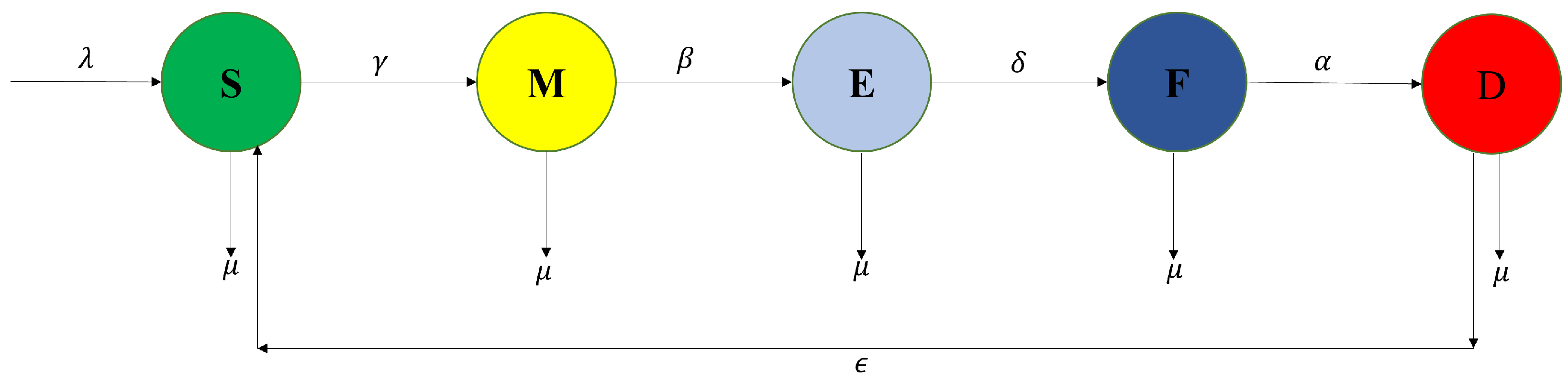In discussing the essential details and necessary steps for setting up and executing a PRCC analysis for a divorce model, we first outline the parameter ranges for each variable $(\lambda ,\gamma ,\beta ,\delta ,\alpha ,ϵ,\mu )$, ensuring these ranges realistically reflect expected system fluctuations. Next, we specify the initial population sizes for each compartment (S, M, E, F, and D). The simulation configuration includes determining the duration and the increment size for numerical integration. Additionally, we establish the desired number of Monte Carlo samples, typically 1000, to ensure statistical robustness. The MATLAB software 9.8.0.1323502 (R2020a) programming environment is also used for conducting simulations and PRCC computations. We then determine relevant model outputs for correlation analysis, such as the ultimate count of individuals who have gone through a divorce, denoted as $D\left(t\right)$. With these components established, parameter sets are sampled based on defined probability distributions, and simulations are conducted for each configuration to generate output data. The process involves computing rankings of parameters and outputs and calculating the PRCC values to assess the sensitivity of model outputs to individual parameters, accounting for the influence of all other factors.

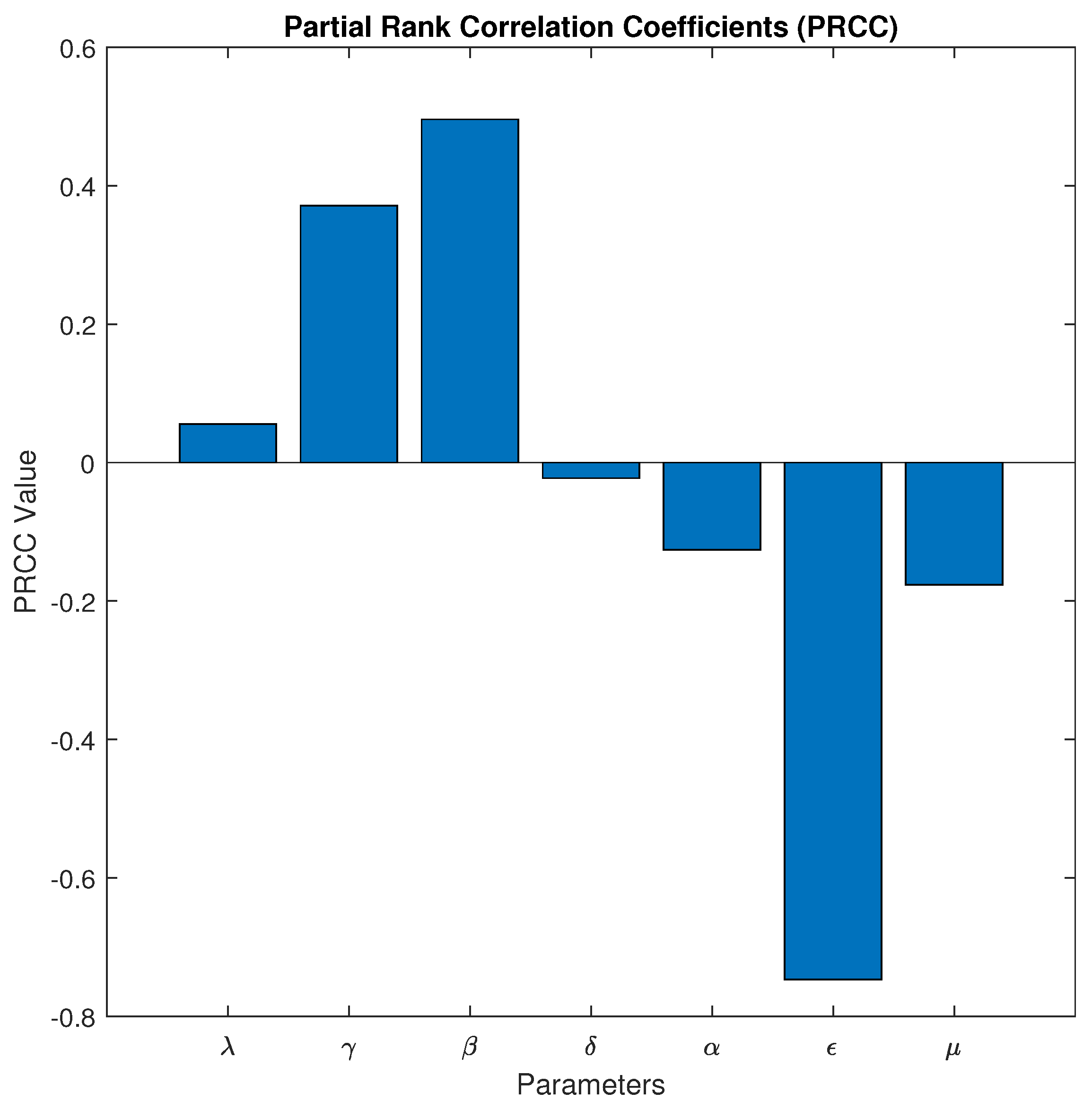
The PRCC shown in Figure 3 reveals the individual impacts of different model parameters on the divorce model’s outcome $D\left(t\right)$. The recruitment rate ($\lambda$) and the rate of short breakup individuals moving to a long breakup ($\delta$) exhibit negative correlations, implying that an increase in these rates leads to a decrease in the outcome variable $D\left(t\right)$. This suggests a potential stabilization or decline in the progression through the stages of the model. Conversely, there is a positive relationship between the rate at which single individuals get married ($\gamma$) and the contact rate between married and divorced individuals ($\beta$). This means that higher rates of marriage and contact accelerate or strengthen the modeled processes, potentially resulting in more transitions between states. Significantly, the divorce rate ($\alpha$) and the natural death rate ($\mu$) have notable negative effects on individuals who have long breakups. This implies that these parameters may function as inhibiting factors in the model dynamics, potentially slowing down or decreasing the number of transitions into the divorce or death states. This research facilitates the comprehension of the most relevant elements and their impact on the behavior of the system, offering a quantitative foundation for targeted interventions or more exploratory studies.

Figure 3. PRCC values against parameters’ values.

6. Numerical Results and Discussion

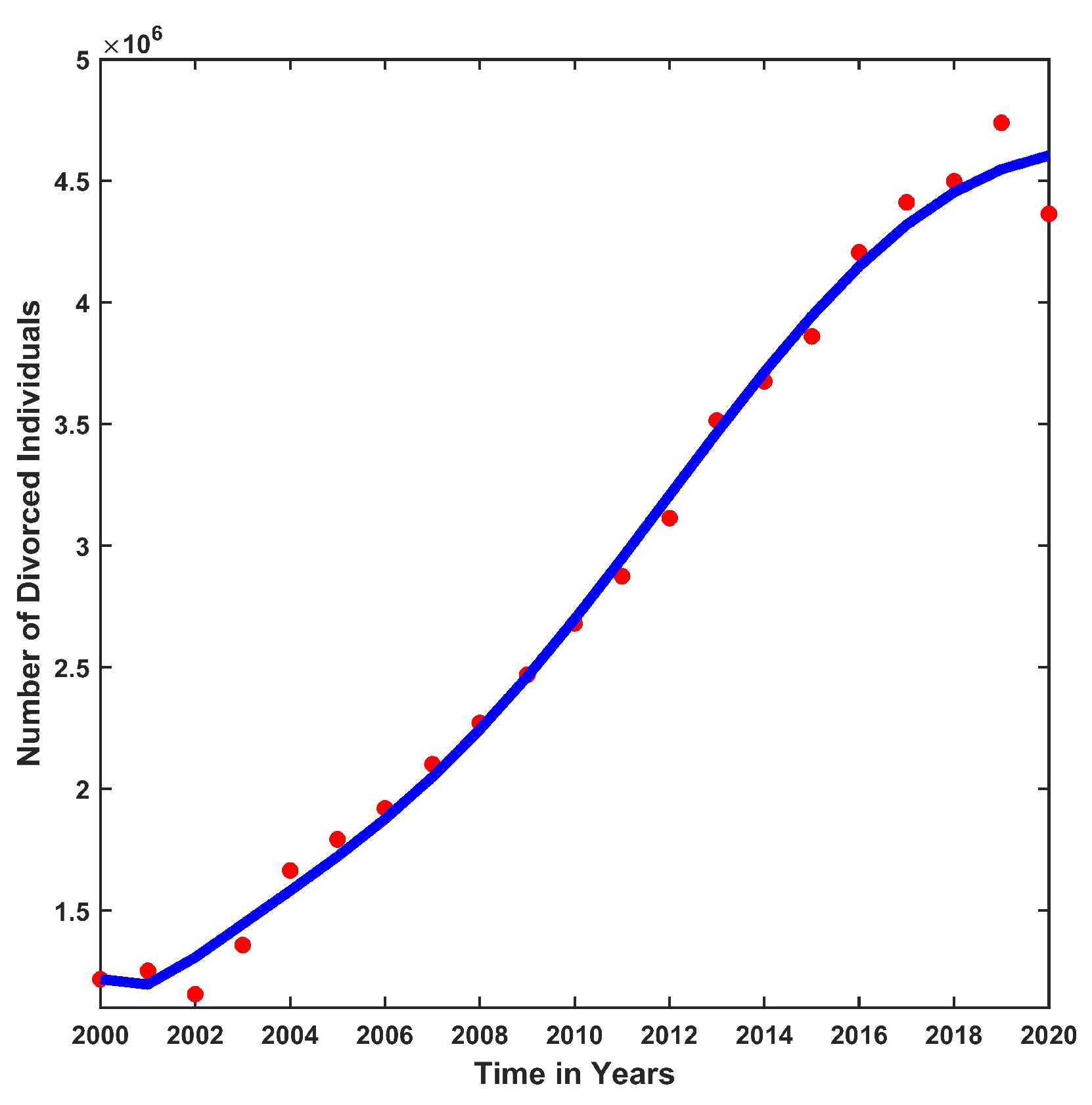
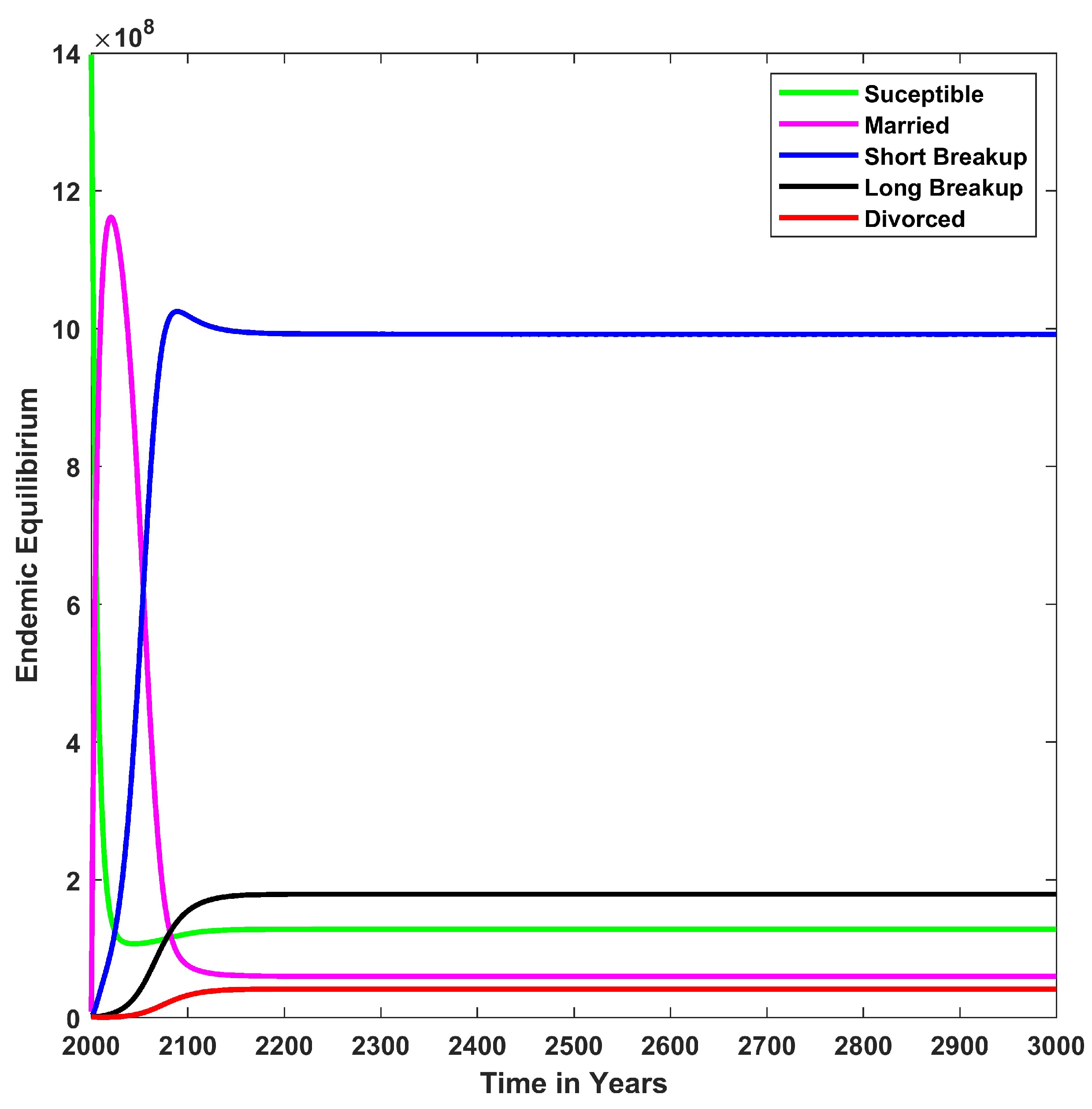
The numerical results provide a comprehensive understanding of divorce trends in China. The population of China stands at 1,411,800,060 [23]. Initially, the population classes are assumed to be: $S\left(0\right)$ = 1,397,291,546, M(0) = 8,491,781, E(0) = 3,000,000, $F\left(0\right)$ = 1,800,000, and $D\left(0\right)$ = 1,216,733. 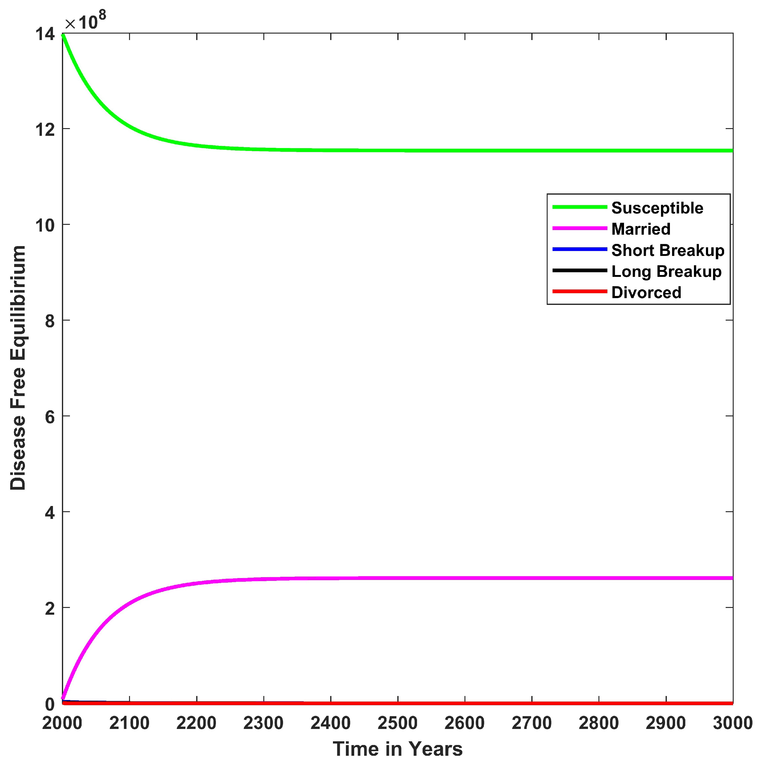The numerical values, fitted using real data, indicate that when ${\mathcal{R}}_0>1$, the solution converges to the endemic equilibrium at $E_1$, as depicted in Figure 4. Conversely, numerical simulations show that when ${\mathcal{R}}_0<1$, the solution converges to the disease-free equilibrium $Z_0$, as shown in Figure 5. 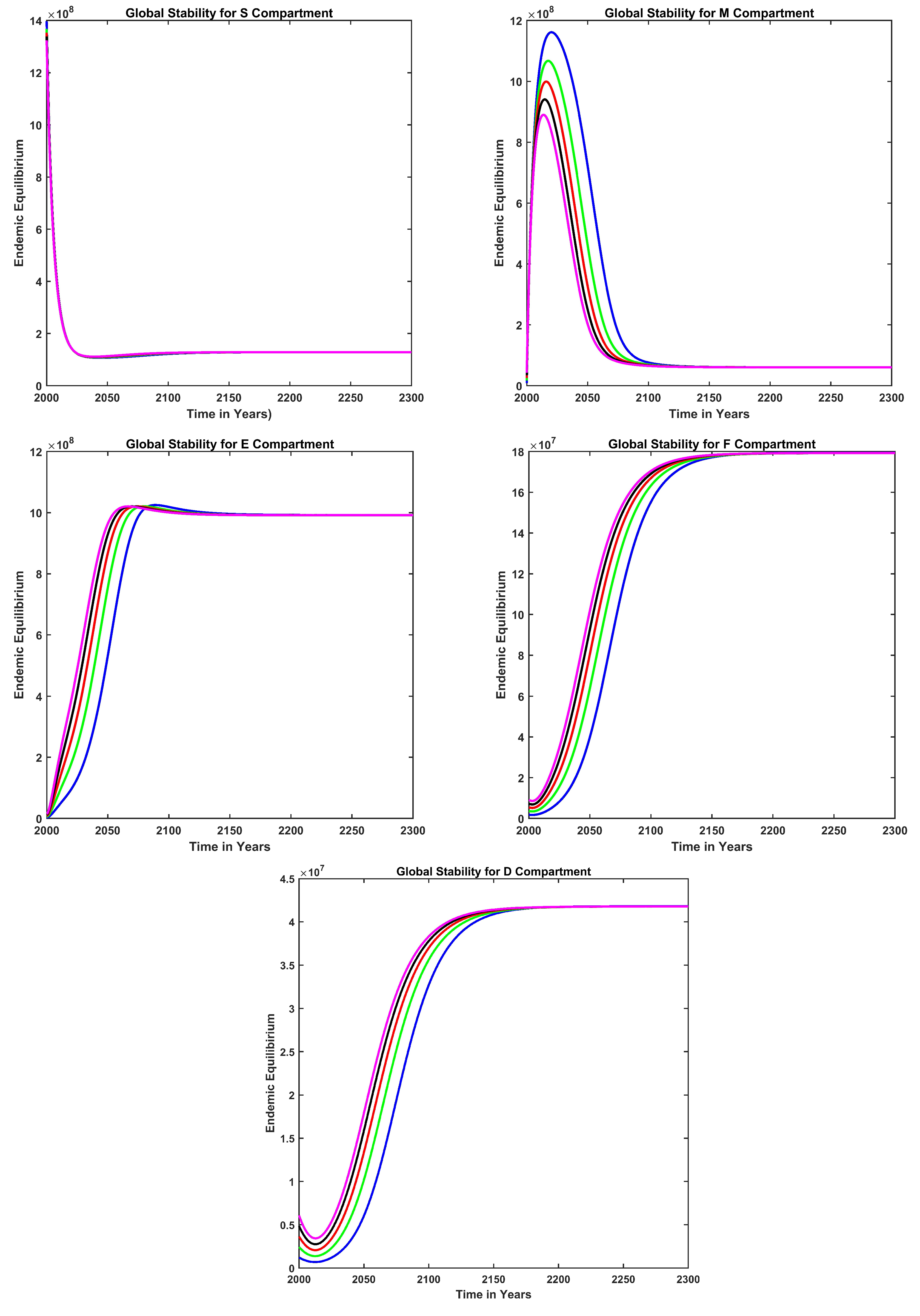Therefore, the system is locally stable, as evident in Figure 4 and Figure 5. 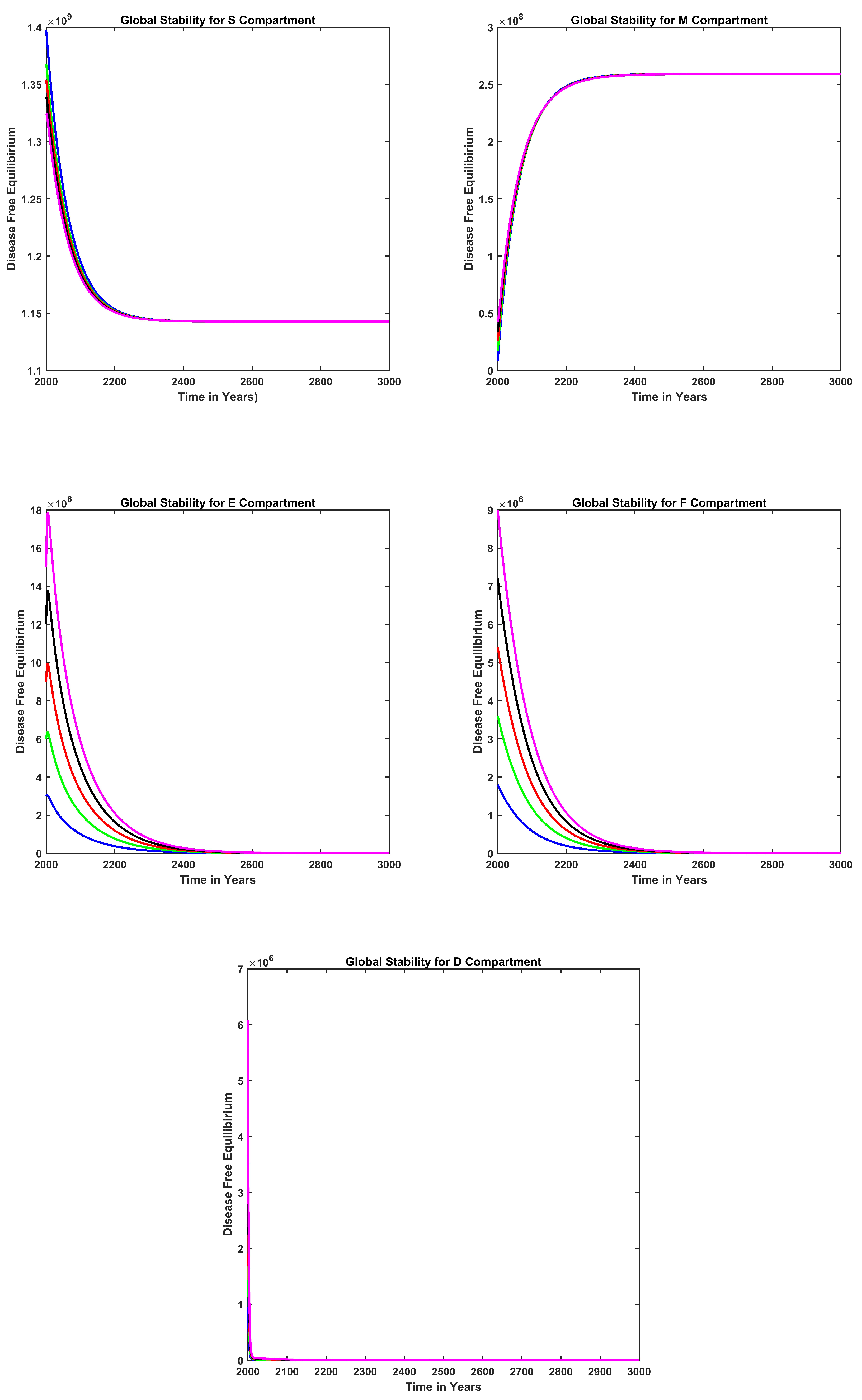Furthermore, under different initial conditions with ${\mathcal{R}}_0>1$ (Figure 6), all the solutions converge to the endemic equilibrium at $E_1$, whereas with ${\mathcal{R}}_0<1$ (Figure 7), all the solutions converge to the disease-free equilibrium $Z_0$. Therefore, the system is globally stable, as evident in Figure 6 and Figure 7.

Figure 4. Dynamical behavior of the proposed model’s compartments when ${\mathcal{R}}_0>1$.

Figure 5. Dynamical behavior of the proposed model’s compartments when ${\mathcal{R}}_0<1$.

Figure 6. The global stability of the proposed model’s compartments when ${\mathcal{R}}_0>1$.

Figure 7. The global stability of the proposed model’s compartments when ${\mathcal{R}}_0<1$.

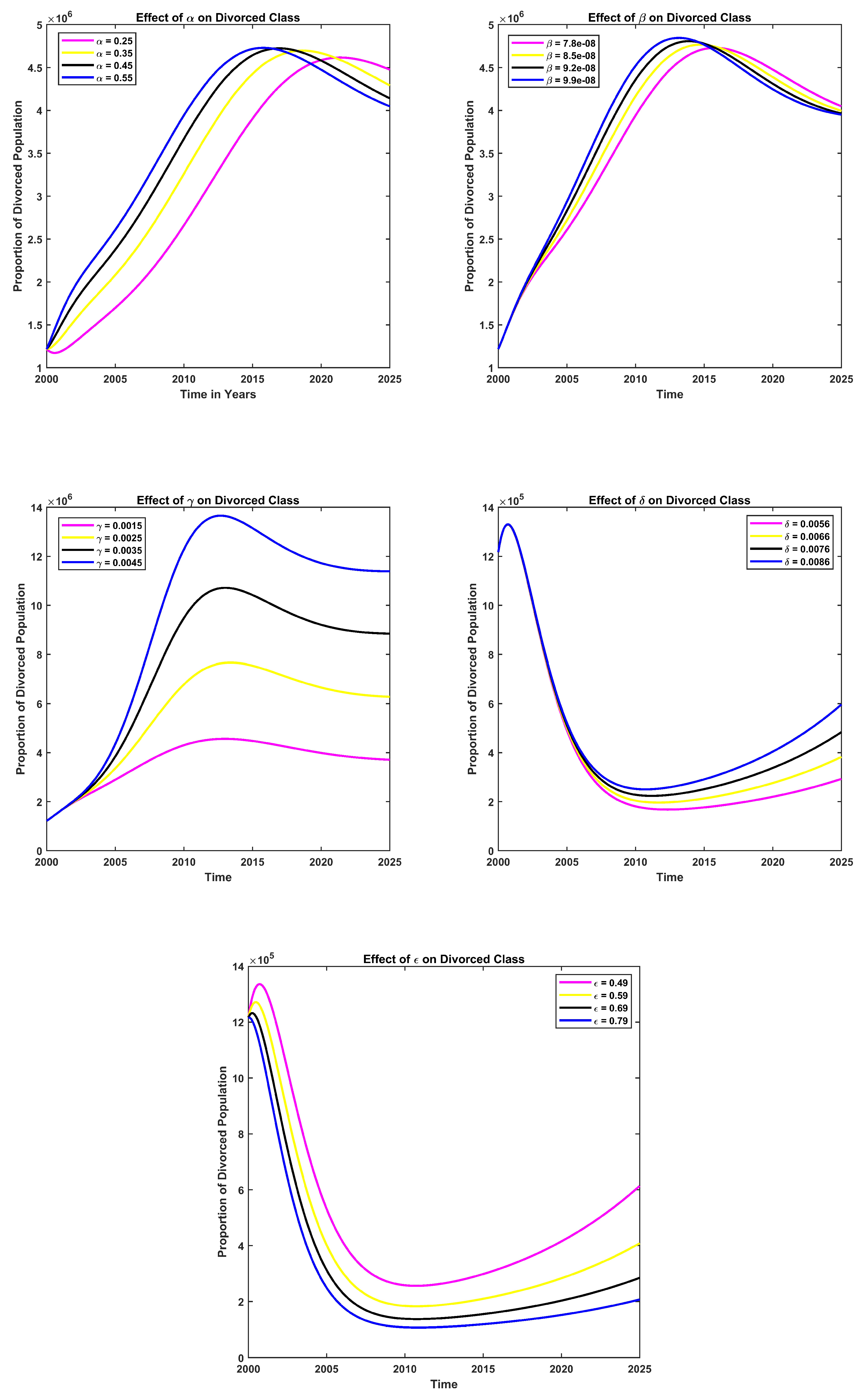
The impacts of various parameters are illustrated in Figure 8. For instance, the effect of $\alpha$ on the divorced class is depicted first and clearly demonstrates that an increase in $\alpha$ leads to a higher divorce rate. Similarly, the effects of $\beta$, $\gamma$, and $\delta$ are observed. In contrast, the effect of $ϵ$ on the divorced class is shown, where an increase in $ϵ$ results in a decrease in the divorce rate.

Figure 8. The plot shows the effects of $\alpha$, $\beta$, $\gamma$, $\delta$, and $ϵ$ when ${\mathcal{R}}_0>1$.

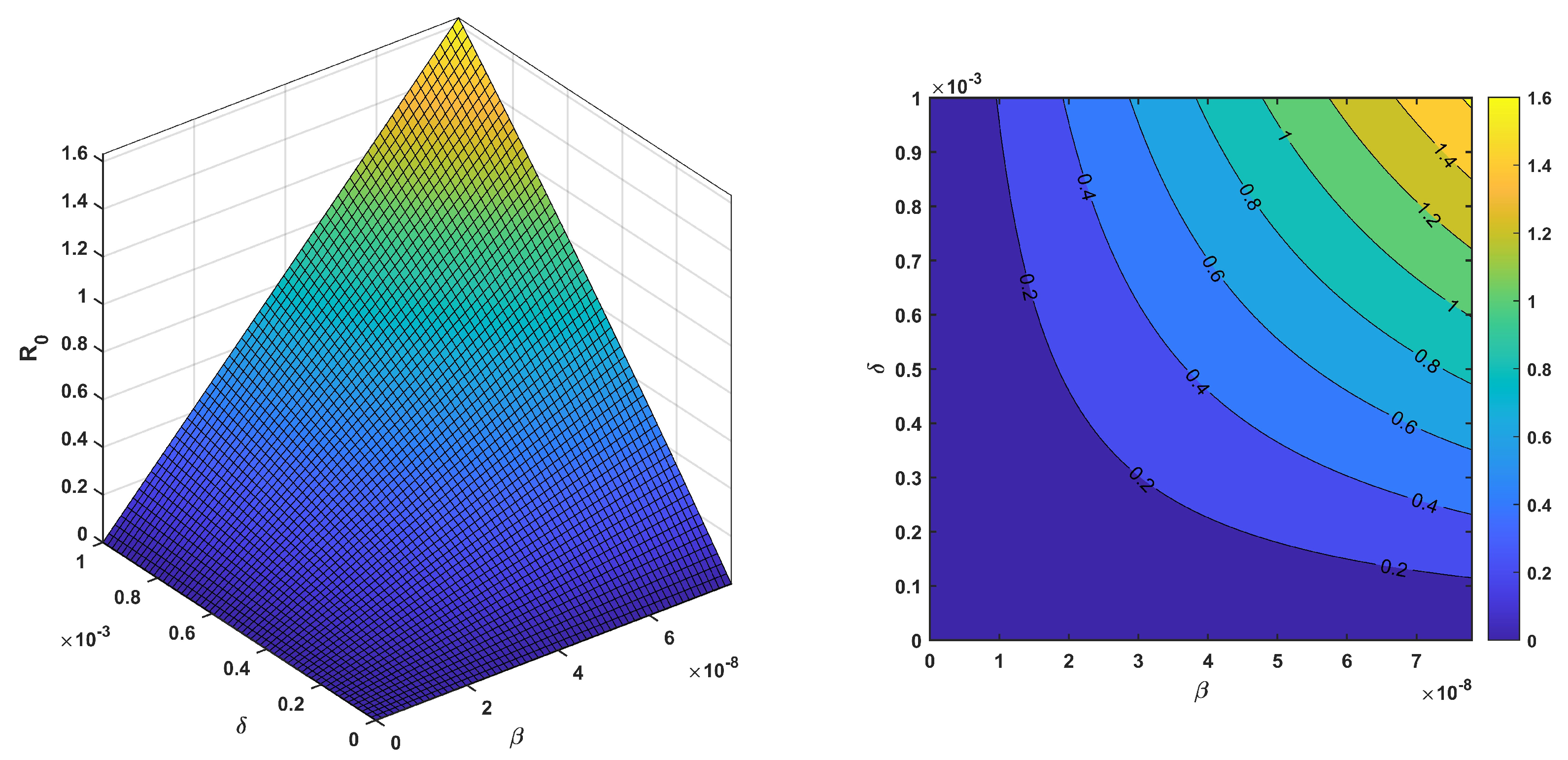
Figure 9 shows two different types of plots related to ${\mathcal{R}}_0$ for the proposed divorce epidemic. The quantity ${\mathcal{R}}_0$ represents the expected number of cases directly generated by one case in a population in which all individuals are susceptible to divorce. The first plot on the left in Figure 9 is a three-dimensional surface plot that shows the relationship between ${\mathcal{R}}_0$, the contact rate ($\beta$), and the divorce rate ($\alpha$). The parameter $\beta$ is represented on the horizontal axis and ranges from 0 to 1, and $\alpha$ is represented on the depth axis and ranges from 0 to 0.001. The vertical axis represents ${\mathcal{R}}_0$, which appears to increase as either $\beta$ or $\alpha$ increases. This suggests that higher contact rates or divorce rates both lead to a higher ${\mathcal{R}}_0$, indicating a more severe potential outbreak.

Figure 9. Cumulative effects of $\beta$ and $\alpha$ on ${\mathcal{R}}_0$ for the proposed divorce model.

The second plot on the right in Figure 9 is a contour plot that provides a top-down view of the same data, projecting the three-dimensional relationship onto two dimensions. The color scale on the right side of the plot indicates the values of ${\mathcal{R}}_0$ corresponding to the colors on the plot. The contour lines represent different levels of ${\mathcal{R}}_0$, showing how combinations of $\beta$ and $\alpha$ correspond to the same ${\mathcal{R}}_0$. In regions where the contour lines are close together, small changes in $\beta$ or $\alpha$ result in large changes in ${\mathcal{R}}_0$, indicating sensitive areas of the parameter space where control measures could have significant impacts on the spread of divorce.

In Figure 9, it can be observed that ${\mathcal{R}}_0$ increases when $\beta$ and $\alpha$ increase. If $\beta$ increases but $\eta$ is very small, then ${\mathcal{R}}_0$ is small and vice versa. Both plots are valuable for understanding how changes in the contact rate and divorce rate impact the spread of divorce. Such models are crucial for public health planning and interventions, allowing experts to simulate various scenarios and formulate strategies to control or prevent outbreaks. 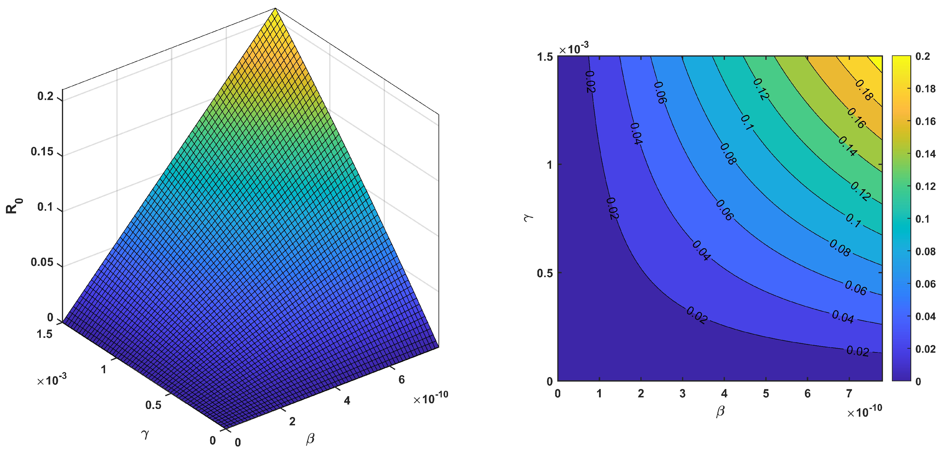In Figure 10, it can be observed that ${\mathcal{R}}_0$ increases when $\beta$ and $\delta$ both increase. If $\beta$ increases and $\delta$ is very low, then ${\mathcal{R}}_0$ is smaller and vice versa. 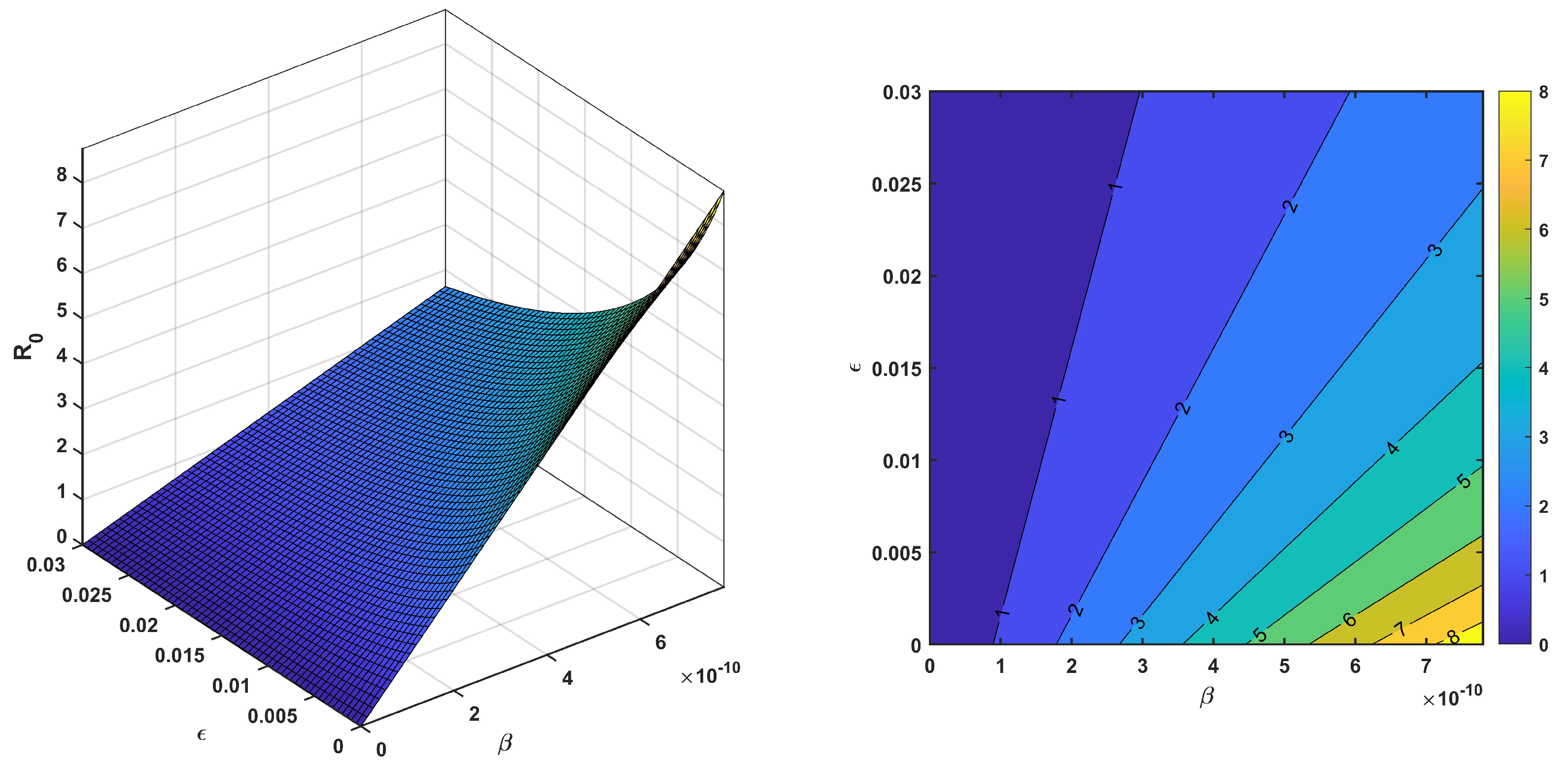In Figure 11, it can be observed that ${\mathcal{R}}_0$ increases when $\beta$ and $\gamma$ both increase. If $\beta$ increases and $\gamma$ is very low, then ${\mathcal{R}}_0$ is smaller. In Figure 12, it can be observed that ${\mathcal{R}}_0$ decreases when $\beta$ and $ϵ$ both increase. Therefore, the parameter $ϵ$ plays a vital role in controlling divorce, as if $\beta$ increases, then divorce can still be controlled. In Figure 13, it can be observed that ${\mathcal{R}}_0$ decreases when $ϵ$ increases, whereas if $\alpha$ increases, then ${\mathcal{R}}_0$ also increases. If $\alpha$ and $ϵ$ both increase, then ${\mathcal{R}}_0$ is smaller. Therefore, $ϵ$ plays a vital role in controlling divorce, as if $\alpha$ increases, then divorce can still be controlled due to $ϵ$.

Figure 10. Cumulative effects of $\beta$ and $\delta$ on ${\mathcal{R}}_0$ for the proposed divorce model.

Figure 11. Cumulative effects of $\beta$ and $\gamma$ on ${\mathcal{R}}_0$ for the proposed divorce model.

Figure 12. Cumulative effects of $\beta$ and $ϵ$ on ${\mathcal{R}}_0$ for the proposed divorce model.

Figure 13. Cumulative effects of $\alpha$ and $ϵ$ on ${\mathcal{R}}_0$ for the proposed divorce model.

7. Conclusions and Future Remarks

In this study, we developed a deterministic model to analyze the dynamics of divorce transmission by utilizing a system of nonlinear ODEs. By employing real data from China spanning the years 2000 to 2020, as reported by Statista, we estimated the model parameters effectively. The number ${\mathcal{R}}_0$, a pivotal metric in our analysis, was derived using the next-generation matrix method. This model demonstrates both local and global asymptotic stability at disease-free and endemic equilibria.

Significantly, our findings underscore the critical role of ${\mathcal{R}}_0$ in the potential for divorce to become epidemic; values above one predict widespread transmission, while values below one suggest containment. Among the parameters, $\beta$ proved to be highly influential, whereas $\alpha$ and $\delta$ exhibited a positive impact on ${\mathcal{R}}_0$. Conversely, $ϵ$ tended to reduce ${\mathcal{R}}_0$. A key objective derived from this understanding is to strategically lower ${\mathcal{R}}_0$ to mitigate the spread of divorce. Our proposed strategies include reducing contact rates between single and married individuals and enhancing the propensity for remarriage among divorced individuals. Theoretical predictions were supported by numerical simulations, which are visually represented to validate the analytical outcomes.

For future research, it would be advantageous to explore the impact of sociocultural factors on the transmission dynamics of divorce. Additional parameters, such as the effects of legal and psychological support systems, could be integrated into the model to provide a more comprehensive understanding. Moreover, comparative studies involving data from different regions or countries could shed light on global patterns and the effectiveness of various intervention strategies. Through such endeavors, we can further refine our model and contribute to more effective societal strategies to manage and possibly reduce the incidence of divorce.

References

- Amato, P.R.; Previti, D. People’s reasons for divorcing: Gender, social class, the life course, and adjustment. J. Fam. Issues 2003, 24, 602–626. [Google Scholar] [CrossRef]
- Copen, C.E.; Daniels, K.; Vespa, J.; Mosher, W.D. First marriages in the United States: Data from the 2006–2010 national survey of family growth. Nat. Health Stat. Rep. 2012, 1–22. [Google Scholar]
- Amato, P.R. The Consequences of Divorce for Adults and Children: An update. J. Marriage Fam. 2000, 62, 1269–1287. [Google Scholar] [CrossRef]
- Kelly, J.B.; Emery, R.E. Children’s adjustment Following divorce: Risk and resilience perspectives. Fam. Relations 2003, 52, 352–362. [Google Scholar] [CrossRef]
- Musa, S.S.; Zhao, S.; Abdulrashid, I.; Qureshi, S.; Colubri, A.; He, D. Evaluating the spike in the symptomatic proportion of SARS-CoV-2 in China in December 2022 considering variolation effects: A modeling analysis. Infect. Dis. Model. 2024, 9, 601–617. [Google Scholar] [CrossRef] [PubMed]
- Naik, P.A.; Qureshi, M.A.; Ahmed, R.; Qureshi, S.; Huang, Z. Stability and bifurcation analysis of a discrete predator-prey system of Ricker type with refuge effect. Math. Biosci. Eng. 2024, 21, 4554–4586. [Google Scholar] [CrossRef] [PubMed]
- Tassaddiq, A.; Shaikh, A.A.; Soomro, A.; Arqub, O.A.; Senol, M. Comparative analysis of classical and Caputo models for COVID-19 spread: Vaccination and stability assessment. Fixed Point Theory Algorithms Sci. Eng. 2024, 2024, 2. [Google Scholar] [CrossRef]
- Gottman, J.M.; Swanson, C.; Murray, J. The mathematics of marital conflict: Dynamic mathematical nonlinear modeling of newlywed marital interaction. J. Fam. Psychol. 1999, 13, 3–19. [Google Scholar] [CrossRef]
- Kenny, D.A.; Kashy, D.A.; Cook, W.L. The Analysis of Dyadic Data; The Guilford Press: New York, NY, USA, 2006. [Google Scholar]
- China: Divorce rate 2022|Statista. Statista. Available online: https://www.statista.com/statistics/279449/divorce-rate-in-china/ (accessed on 20 February 2024).
- Zoladek, H.; Murillo, R. Qualitative Theory of ODEs: An Introduction to Dynamical Systems Theory; World Scientific, 2022. [Google Scholar]
- Grossman, S.I.; Derrick, W.R. Elementary Differential Equations with Applications; Addison-Wesley Publishing Company: Reading, MA, USA, 1981. [Google Scholar]
- Hernandez-Suarez, C.; Lopez, O.M. A simple and intuitive method to calculate R0 in complex epidemic models. arXiv 2022, arXiv:2208.11509. [Google Scholar] [CrossRef]
- Perasso, A. An introduction to the basic reproduction number in mathematical epidemiology. ESAIM 2018, 62, 123–138. [Google Scholar] [CrossRef]
- Van Den Driessche, P.; Watmough, J. Reproduction numbers and sub-threshold endemic equilibria for compartmental models of disease transmission. Math. Biosci. 2002, 180, 29–48. [Google Scholar] [CrossRef] [PubMed]
- La Salle, J.P. The Stability of Dynamical Systems; Society for Industrial and Applied Mathematics: Philadelphia, PA, USA, 1976. [Google Scholar] [CrossRef]
- Rand, D. Mapping global sensitivity of cellular network dynamics: Sensitivity heat maps and a global summation law. J. R. Soc. Interface 2008, 5. [Google Scholar] [CrossRef] [PubMed]
- Marino, S.; Hogue, I.B.; Ray, J.C.J.; Kirschner, D.E. A methodology for performing global uncertainty and sensitivity analysis in systems biology. J. Theor. Biol. 2008, 254, 178–196. [Google Scholar] [CrossRef] [PubMed]
- Helton, J.C.; Davis, F. Illustration of Sampling-Based Methods for Uncertainty and sensitivity analysis. Risk Anal. 2002, 22, 591–622. [Google Scholar] [CrossRef] [PubMed]
- Morris, M.D. Factorial sampling plans for preliminary computational experiments. Technometrics 1991, 33, 161–174. [Google Scholar] [CrossRef]
- Sobol, I.M. On sensitivity estimation for nonlinear mathematical models. Matem. Mod. 1990, 2, 112–118. [Google Scholar]
- Berhe, H.W.; Makinde, O.D.; Theuri, D.M. Parameter estimation and sensitivity analysis of Dysentery Diarrhea Epidemic model. J. Appl. Math. 2019, 2019, 1–13. [Google Scholar] [CrossRef]
- People’s Republic of China-Place Explorer-Data Commons. Available online: https://datacommons.org/place/country/CHN?utm%20medium=explore&mprop=count&%20popt=Person&hl=en] (accessed on 17 April 2024).
Disclaimer/Publisher’s Note: The statements, opinions and data contained in all publications are solely those of the individual author(s) and contributor(s) and not of MDPI and/or the editor(s). MDPI and/or the editor(s) disclaim responsibility for any injury to people or property resulting from any ideas, methods, instructions or products referred to in the content.  |
© 2024 by the authors. Licensee MDPI, Basel, Switzerland. This article is an open access article distributed under the terms and conditions of the Creative Commons Attribution (CC BY) license (https://creativecommons.org/licenses/by/4.0/).