This section recalls the framework of the projection methods used for solving the Navier–Stokes equations in incompressible flow simulations, also known in the literature as the fractional step method.
5.1. Model and Algorithm
This method broadly falls into three schemes: pressure-correction, velocity-correction, and consistent splitting methods. In particular, some steps present in the projection algorithm are essentially the same as the orthogonal decomposition of the velocity. Therefore, since the decomposition is treated by using the mixed finite element tools presented in
Section 3.3, we establish a connection to fully resolve the Navier–Stokes system of equations. For an exhaustive review of this method, the interested reader can consult the work of Guermond et al. [
23].
The projection method originates from the incompressibility constraint, which represents the main motivation of this work. In particular, one of the main issues related to the numerical solution of momentum and mass conservation equations is the coupling between velocity and pressure, imposed by the condition of zero divergence of velocity. The solution of the coupled velocity–pressure system can be expensive from a computational point of view, and this has led to the development of different numerical algorithms for the treatment of the split system for velocity and the pressure fields. In order to overcome these problems, many authors introduced the projection method by which the Navier–Stokes system is subdivided into two separate steps, one for the velocity and one for the pressure.
The first idea that appeared in the literature is related to the work of Chorin and Temam [
21,
22], where the time-dependent solution of incompressible viscous flow has been proposed. Specifically, the idea is to build a sequence of decoupled elliptic equations for the velocity and the pressure and solve them at each time step. Indeed, this numerical method leads to an efficient simulation and reduces the computational effort.
Hereafter, the algorithm employed for the resolution of the Navier–Stokes system in the multigrid finite element library FEMuS [
41] is described, considering the standard incremental pressure correction scheme. Thus, we recall the Navier–Stokes system for a generic incompressible fluid flow, with constant physical properties and a smooth force
where homogeneous Dirichlet boundary conditions are taken into account.
In order to define the time-dependent solutions, we can consider the time step
and set
for
, where
T is the upper bound of the time interval considered,
. To describe the adopted pressure–velocity split algorithm, the simple Euler scheme for the time discretization is used. Specifically, a fictitious intermediate velocity field
is introduced, leading to
After that, following a standard approach, the equation can be subdivided into two different equations by introducing the incremental pressure
, and considering
,
The first equation considers the viscous effect solving the velocity , which has a divergence different from zero, while the second equation represents the projection between the two velocity fields, where the constraint is understood.
In this work, a different velocity–pressure split is proposed and analyzed with the objective of exploiting the orthogonal decomposition of the velocity field [
42]. Specifically, the first equation, which solves the intermediate velocity
, remains the same, while the pressure equation is not transformed by applying the divergence operator as in standard split algorithms. Thus, for the ‘pressure equation’, we solve directly the coupled system
In this way, we avoid the resolution of the Poisson equation for the incremental pressure, which would affect the imposition of the well-known non-physical homogeneous Neumann boundary condition for .
Therefore, we apply the orthogonal decomposition to (
54) by using the properties of the Raviart–Thomas finite element family. In particular, (
54) is solved by considering the same optimal minimization problem presented for the multiphase flow problem (
36). The objective is to find a field
which is the closest velocity to
under the constraint of the divergence equal to zero.
Differently, for the velocity
the solution space can be found considering the standard solution of the Navier–Stokes equations. In particular, consider the Taylor–Hood finite element space
. Thus, if we have
, the objective is to find the velocity
by minimizing
over the linear function subspace
.
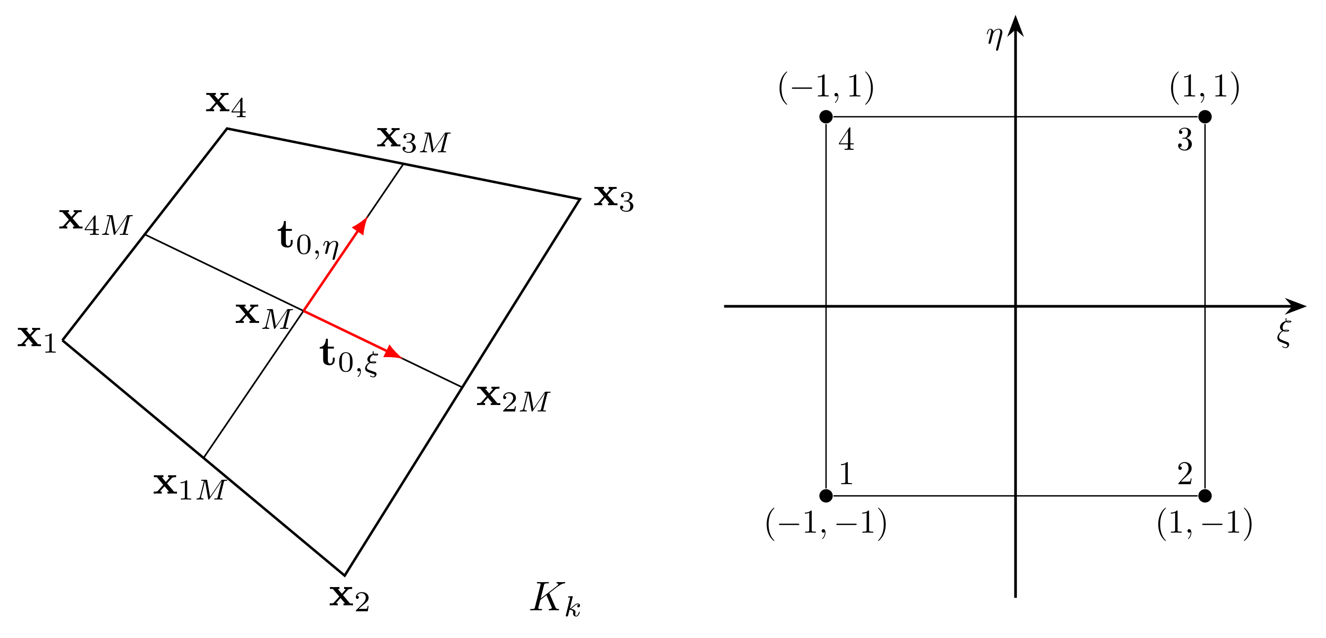
Naturally, for , the velocity approximation is defined as , where is the velocity field at the points j and indicates the Lagrangian quadratic polynomial basis functions. Instead, for , the approximation velocity reads as , where represents the fluxes through the faces and corresponds to the Raviart–Thomas vector basis functions.
In order to derive the final system to be solved, we can consider now a piecewise constant pressure, i.e.,
. Therefore, the system to be solved is described with the following two equations:
where
can be interpreted as the discrete Lagrange multiplier of the divergence equation.
It is worth noting that (
56) is only a step of the split algorithm. Indeed, the elliptic equation for the velocity
in (
52) is still solved by considering standard Lagrangian finite elements, in particular the Taylor–Hood type in our case.
We recall that by using the lowest-order element the velocity is determined considering only the fluxes through the element edges, i.e., four (six) degrees of freedom for a bidimensional (three-dimensional) domain. Naturally, in this discussion, only quadrilateral and hexahedral elements have been considered. Hence, the local matrix is equipped only with five (seven) rows that represent the four (six) fluxes through the faces and the central value for the pressure field, instead of using, for example, the nine nodes of a biquadratic quadrilateral with Lagrangian basis functions.
5.2. Numerical Tests
In this section, we aim to test the employment of the Raviart–Thomas finite element family in the framework of the projection method for the resolution of the Navier–Stokes equation. Specifically, (
56) was adopted, where we recall that the orthogonal decomposition of the velocity field is considered as the second step of the split algorithm, i.e., the resolution of the pressure equation.
Three cases were investigated, considering a bidimensional and a three-dimensional geometry: a channel, in both two and three dimensions, and a bidimensional cavity. For these tests, the same comparison was performed, considering three different algorithms for the numerical solution. The first one consists of a standard coupled algorithm for the resolution of the velocity and pressure and by using classical Lagrangian finite elements for the field discretization. The second technique is based on the same finite element family but employs a standard projection algorithm for the Navier–Stokes system. Lastly, the third method is characterized by the employment of the Raviart–Thomas finite element family for the resolution of the pressure equation in the context of the split technique.
The first analyzed case focuses on the resolution of the Navier–Stokes equation characterized by a low Reynolds number inside a bidimensional channel, i.e., a laminar flow. It is well-known that the solution of this kind of configuration is expressed by the Poiseuille profile for the streamwise component of the velocity. Indeed, we expect to obtain the classical parabolic profile.
In
Figure 6, the investigated mesh discretizations of the channel geometry are reported. Note that on the right is reported a channel discretization where non-affine elements have been employed. On the other hand, the multigrid refinement produces elements that converge to a parallelogram shape, which is an affine element since the opposite edges are parallel, avoiding any convergence issue well documented in the literature [
43,
44].
Considering the boundary conditions, at the inlet section
, a fixed velocity was imposed, a standard no-slip boundary condition was imposed on the wall-side
, while an outlet-type condition was imposed at the outlet section
to fix the pressure value. For this kind of numerical simulation, it is not possible to have an analytical solution of the velocity field. In fact, even though a Poiseuille flow type is searched, if we consider an inlet boundary condition, the analytical solution for the Navier–Stokes system does not exist. For this reason, the velocity error norm with respect to a reference solution does not have numerical significance. On the other hand, in order to compare qualitatively the solutions with the three types of numerical discretizations, the
norm of the velocity field over the entire domain is reported for different grid refinements. In particular, for both regular and irregular meshes, we compute the velocity norm as reported in
Table 3. The different methods are denoted with
,
, respectively, for the coupled and split technique with Taylor–Hood finite elements and with
for Raviart–Thomas finite elements.
We can notice that with the increasing of the grid refinement, the velocity norm values tend to the same value for every method, ensuring reliable numerical results for this test. Consider that even if the second mesh is characterized by non-affine quadrilateral elements, the numerical solution is sought considering a multigrid approach. Therefore, the initial irregular mesh tends to asymptotically affine quadrilateral elements, allowing the use of the standard Raviart–Thomas family of order 0. The last column of
Table 3 confirms that with this geometry, this spatial discretization is able to find the right numerical solution.
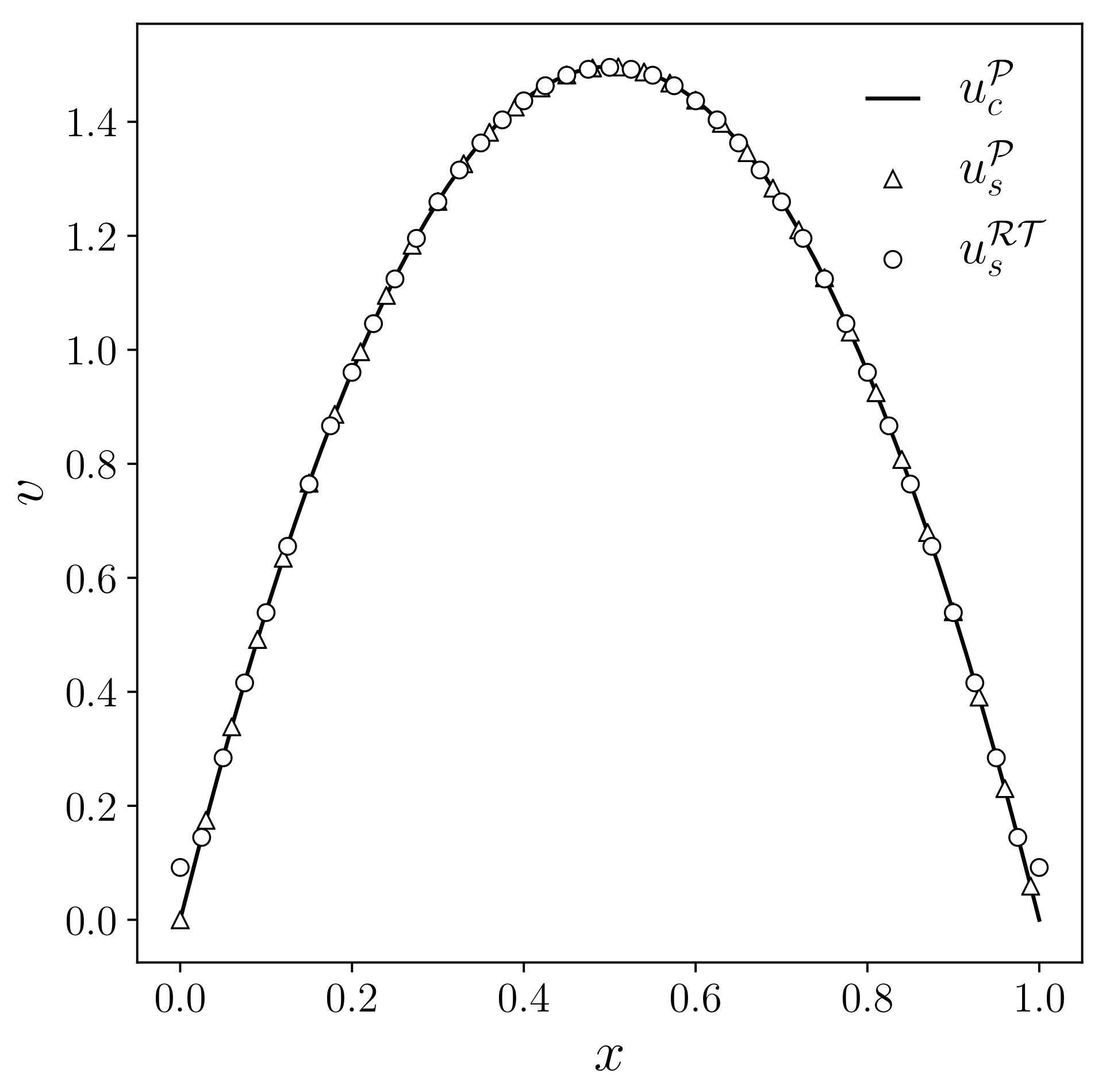
In addition, considering the framework of a laminar flow inside a channel, the main variable of interest is the streamwise component of the velocity field, denoted with
v. For this reason, in
Figure 7, the velocity profile of
v is reported for the three different algorithms as a function of the
x coordinates. The plot has been performed considering a fixed
y equal to 1. Since the numerical solutions between the two different grids are very similar, we report only the case with regular quadrilateral elements.
Considering
Figure 7, the type of algorithm to solve the Navier–Stokes system is denoted with the subscript,
c for the coupled system and
s for the split one. With the superscript is denoted the type of finite element family employed for the velocity–pressure discretization,
for standard
Lagrangian elements and
the Raviart–Thomas elements. The solid line represents the reference numerical result, that is, the numerical solution obtained with a coupled algorithm and classical Taylor–Hood Lagrangian elements. With the markers, the numerical solutions of the split system are reported: the triangular markers represent the case where
elements were employed in every equation, while the circular markers represent the solution obtained by using an
approximation for the resolution of the pressure equation. We can notice a good agreement of the velocity profiles obtained by employing the three different algorithms.
In the second test, we want to verify the convergence error rate by considering a cavity configuration, i.e., a rectangular closed geometry. Specifically, the domain is described with the same channel as the previous cases, i.e., the bidimensional channel described in
Figure 6, where the elements employed for the spatial discretization are standard regular quadrilateral elements. Regarding the velocity field, the boundary condition imposed on every edge is a homogeneous Dirichlet boundary condition in order to have
on the walls.
In order to compute the
norm of the velocity error, the steady exact Navier–Stokes solution was imposed on the right-hand side of the equation. In fact, given a generic operator
A which represents the left-hand side terms of the Navier–Stokes equation, we aim to solve
for a specified
, which represents the desired solution. Specifically, the exact solution for the velocity components reads as
In
Table 4, the velocity error norm and the corresponding order of convergence for different levels of refinement are reported for the
finite element approximation. The order of convergence
p is reported in the last column, computed as
. We can notice a linear trend for the velocity error norm, as expected by theoretical error estimates for the Raviart–Thomas velocity approximation.
The same test was also computed considering the standard Taylor–Hood Lagrangian basis function, with both a coupled and a split algorithm. The results are reported in
Table 5. We can notice a good convergence trend for the velocity error for both methods even though the order of convergence
p is not reported. In fact, despite these parameters appearing to be equal to 3 for both simulations, we recall that the velocity error should be considered together with the pressure error norm. For coupled systems or for Lagrangian-type basis functions that are not pointwise divergence-free, we know that an error in the pressure field produces an effect also the error in the velocity.
An interesting result was found considering the behavior of the velocity divergence. As expected, for the coupled system solved by using the
approximation, the velocity divergence reaches values close to machine precision, indicating that this technique is equipped with an exact zero divergence in every point. Considering the other two methods, the results are reported in
Table 6.
It is worth noting that the velocity divergence error is different from zero as expected. On the other hand, these values seem to converge with a quadratic order.
The last test represents the extension of the bidimensional Poiseuille flow to a three-dimensional configuration, i.e., a regular parallelepiped. The considered domain is represented in
Figure 8, where the characteristic lengths have the same values (
and
). Moreover, regular hexahedral elements were employed for the domain discretization.
The flow configuration follows the same path of the bidimensional case, and thus the fluid enters at the inlet section and exits through the outlet section . On the remaining boundaries, the standard no-slip boundary condition was imposed.
Regarding the reliability of the numerical solutions, the same comments of the two-dimensional channel case can also be drawn for the case of a three-dimensional channel. Therefore, since it is not possible to compare the numerical solution with an analytical field, also in this case the
-norm of the velocity field was computed for the three methods as an indicator of the solution goodness. For this reason, in
Table 7 the velocity norm values are reported considering three levels of refinements for the three techniques. The notation is the same as the two-dimensional channel test.
The -norm of the velocity field tends to the same value for each different algorithm, confirming the good behavior of the numerical solution, as already shown in the bidimensional case.
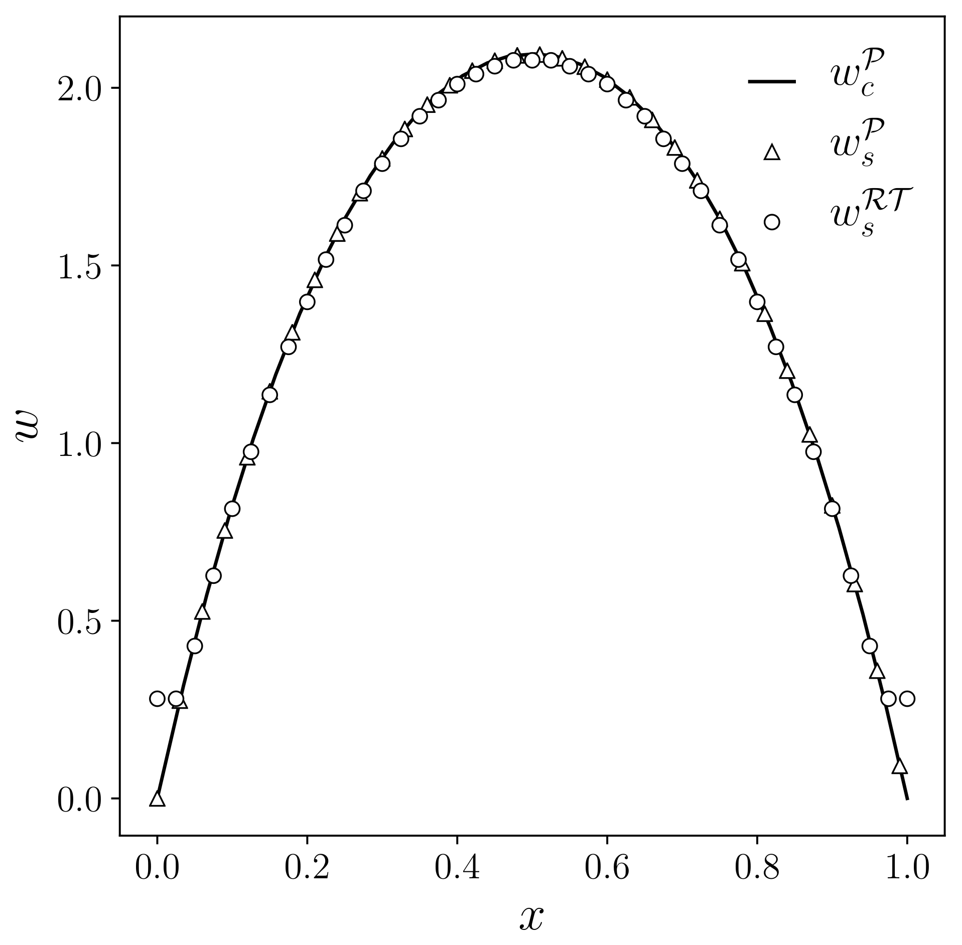
Furthermore, in this case, the same qualitative comparison between three types of algorithms was performed on the numerical solution. Therefore, in
Figure 9 the streamwise velocity component
w is reported, where the employed notation and symbols are the same as the bidimensional channel. The
w component is represented as a function of the
x coordinate, with a plot performed with a fixed
y coordinate equal to
.
Figure 9 shows good accuracy for the computed numerical solution. Indeed, the velocity profile
w obtained with a Raviart–Thomas approximation of the pressure equation in a split system (
56) has a similar trend to the velocity profile obtained with a standard coupled (
50) and split algorithm (
52).


