Strong Stability Preserving Two-Derivative Two-Step Runge-Kutta Methods

Abstract

In this study, we introduce the explicit strong stability preserving (SSP) two-derivative two-step Runge-Kutta (TDTSRK) methods. We propose the order conditions using Albrecht’s approach, comparing to the order conditions expressed in terms of rooted trees, these conditions present a more straightforward form with fewer equations. Furthermore, we develop the SSP theory for the TDTSRK methods under certain assumptions and identify its optimal parameters. We also conduct a comparative analysis of the SSP coefficient among TDTSRK methods, two-derivative Runge-Kutta (TDRK) methods, and Runge-Kutta (RK) methods, both theoretically and numerically. The comparison reveals that the TDTSRK methods in the same order of accuracy have the most effective SSP coefficient. Numerical results demonstrate that the TDTSRK methods are highly efficient in solving the partial differential equation, and the TDTSRK methods can achieve the expected order of accuracy.

1. Introduction

The partial differential equation (PDE) considered in this paper is

$${\displaystyle \frac{\partial y(t,x)}{\partial t}}+{\displaystyle \frac{\partial f\left(y(t,x)\right)}{\partial x}}=0.⟶y_t+f{\left(y\right)}_x=0.$$

(1)

We usually use spatial discretization methods and temporal discretization methods to calculate PDE independently. There are many successful high-order methods used in spatial and temporal discretization [1,2,3]. Numerical robustness directly determines the simulation results in solving the PDE. The numerical stability of temporal discretization schemes also plays a crucial role in the computation of stiff equations [4,5,6], such as the convection-diffusion equation, diffusion-reaction equation. Furthermore, the current research is primarily focused on the development of high-order temporal methods that combine high efficiency with the strong stability preserving (SSP) property [7].

In recent decades, the methods [8,9,10,11] combining multistage, multistep and multiderivative explore the approach to establishing high-order SSP temporal discretization methods [12,13,14,15], in which the order conditions and SSP property for these methods are the main contents of the research. There are two devices to build the order conditions: one is based on the rooted trees theory proposed by Butcher [16,17], and the other is proposed by Albrecht [18], who used the error analysis approach to develop order conditions and introduce their relevance with rooted trees theory. By using rooted trees theory, the researchers have developed the order conditions for two-step RK (TSRK) methods [19], two-derivative RK (TDRK) methods [20] and two-derivative two-step RK (TDTSRK) methods [21]. For Albrecht’s approach, Ketcheson et al. [22] discussed the order conditions for TSRK methods and verified that it has a simpler form than the order conditions in terms of rooted trees. Then, this approach has been utilized to develop the general linear methods (GLMs) [23] and second derivative general linear methods (SGLMs) [24].

For the numerical stability property, the schemes used the A-stability or L-stability [25,26] to desirable stability property in ordinary differential equation (ODE), and focused on the SSP property in PDE. Shu and Osher [3] introduced the concept of SSP methods and built SSP theory for RK methods. Christlieb et al. [27] extended SSP conditions to TDRK methods and displayed the optimal SSP two-stage third-order TDRK (TDRK23) method, two-stage fourth-order TDRK (TDRK24) method, and three-stage fifth-order TDRK (TDRK35) method. Grant et al. [28] developed the SSP theory for TDRK methods by Taylor series conditions. Bresten et al. [29] investigated the SSP property of multistep RK methods. Izzo and Jackiewicz [30] presented the SSP property of GLMs, and compared with TSRK methods and multistep multistage methods. Moradi et al. [31] showed the SSP theory for SGLMs. Besides, the SSP property of the TDTSRK methods has not been studied yet.

In this study, we formulate explicit SSP TDTSRK methods and validate their numerical characteristics. In Section 2, we use Albrecht’s approach to develop the order conditions of the TDTSRK methods, which have simpler equations and fewer equations than the order conditions given by the rooted trees method. Under some assumptions, we develop the SSP theory for the TDTSRK methods, and compare the optimal SSP coefficient with other methods in Section 3. In Section 4, we test SSP property and order of accuracy for different methods, including the TDTSRK, TDRK, and RK methods. The numerical result shows that the TDTSRK methods have the most effective SSP coefficient in the theoretical and numerical results for the same order of accuracy. Conclusions are presented in Section 5.

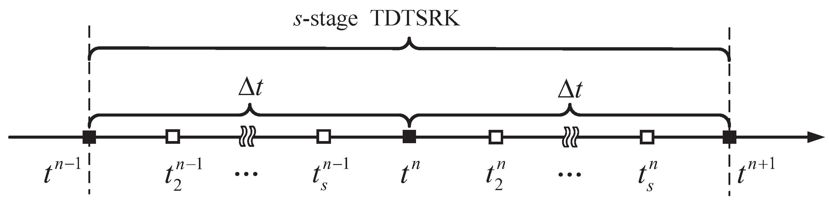
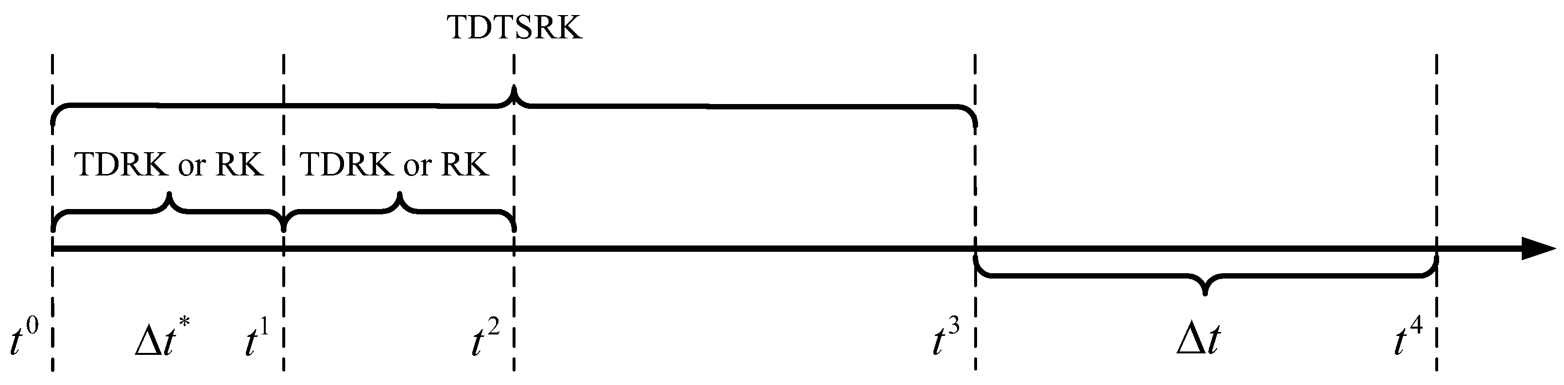
2. Structure of TDTSRK Methods

2.1. Derivation of TDTSRK Methods

For partial differential equation, we use the spatial scheme to calculate the term $F\left(y\right)=-f{\left(y\right)}_x$, and the Equation (1) can be written as the semi-discretized equation

$$y_t=F\left(y\right).$$

(2)

The second derivative of Equation (1) is given by $y_{tt}=G\left(y\right)=F_y\left(y\right)y_t$.

The structure of s-stage TDTSRK scheme is depicted in Figure 1, and the time step size $\Delta t$ is used to discretize the time interval. The $u^n$ is used to denote the value of $y^n$ at the time step $t^n$. The explicit s-stage TDTSRK methods are defined by the following

$$\begin{array}{cc}\hfill y_i^{n-1}& =u^{n-1}+\Delta t\sum _{j=1}^{i-1}{a}_{ij}F\left(y_j^{n-1}\right)+\Delta t^2\sum _{j=1}^{i-1}{\widehat{a}}_{ij}G\left(y_j^{n-1}\right)1\le i\le s,\hfill \\ \hfill y_i^n& =u^n+\Delta t\sum _{j=1}^{i-1}{a}_{ij}F\left(y_j^n\right)+\Delta t^2\sum _{j=1}^{i-1}{\widehat{a}}_{ij}G\left(y_j^n\right)1\le i\le s,\hfill \\ \hfill u^{n+1}& =u^n+\Delta t\sum _{i=1}^s\left(v_{i}F\left(y_i^n\right)+w_{i}F\left(y_i^{n-1}\right)\right)+\Delta t^2\sum _{i=1}^s\left({\widehat{v}}_{i}G\left(y_i^n\right)+{\widehat{w}}_{i}G\left(y_i^{n-1}\right)\right).\hfill \end{array}$$

(3)

We can write the method in the matrix form, and rewrite it into a matrix form by defining

$$\begin{array}{cc}\hfill {\mathit{y}}^{n-1}& =\mathit{e}{u}^{n-1}+\Delta t\mathit{A}{\mathit{F}}^{n-1}+\Delta t^2\widehat{\mathit{A}}{\mathit{G}}^{n-1},\hfill \\ \hfill {\mathit{y}}^n& =\mathit{e}{u}^n+\Delta t\mathit{A}{\mathit{F}}^n+\Delta t^2\widehat{\mathit{A}}{\mathit{G}}^n,\hfill \\ \hfill u^{n+1}& =u^n+\Delta t({\mathit{v}}^T{\mathit{F}}^n+{\mathit{w}}^T{\mathit{F}}^{n-1})+\Delta t^2({\widehat{\mathit{v}}}^T{\mathit{G}}^n+{\widehat{\mathit{w}}}^T{\mathit{G}}^{n-1}),\hfill \end{array}$$

(4)

where the RK matrix $\mathit{A}$, the TDRK matrix $\widehat{\mathit{A}}$, the time stage vectors ${\mathit{y}}^{n-1}$, ${\mathit{y}}^n$, and the weight vectors $\mathit{v}$, $\widehat{\mathit{v}}$, $\mathit{w}$, $\widehat{\mathit{w}}$ can be given by

$$\begin{array}{cc}\hfill {\mathit{y}}^{n-1}=\left(\begin{array}{c}{y}_1^{n-1}\\ y_2^{n-1}\\ ⋮\\ y_s^{n-1}\end{array}\right),{\mathit{y}}^n=\left(\begin{array}{c}{y}_1^n\\ y_2^n\\ ⋮\\ y_s^n\end{array}\right),\mathit{v}=\left(\begin{array}{c}{v}_1\\ v_2\\ ⋮\\ v_s\end{array}\right),\widehat{\mathit{v}}& =\left(\begin{array}{c}{\widehat{v}}_1\\ {\widehat{v}}_2\\ ⋮\\ {\widehat{v}}_s\end{array}\right),\hfill \\ \hfill \mathit{w}=\left(\begin{array}{c}{w}_1\\ w_2\\ ⋮\\ w_s\end{array}\right),\widehat{\mathit{w}}=\left(\begin{array}{c}{\widehat{w}}_1\\ {\widehat{w}}_2\\ ⋮\\ {\widehat{w}}_s\end{array}\right),\mathit{A}=\left(\begin{array}{cccc}0& 0& \cdots & 0\\ a_{21}& 0& \cdots & 0\\ ⋮& ⋮& ⋮& ⋮\\ a_{s1}& a_{s2}& \cdots & 0\end{array}\right),\widehat{\mathit{A}}=& \left(\begin{array}{cccc}0& 0& \cdots & 0\\ {\widehat{a}}_{21}& 0& \cdots & 0\\ ⋮& ⋮& ⋮& ⋮\\ {\widehat{a}}_{s1}& {\widehat{a}}_{s2}& \cdots & 0\end{array}\right),\hfill \end{array}$$

(5)

and the derivatives ${\mathit{F}}^n$, ${\mathit{F}}^{n-1}$, ${\mathit{G}}^n$, ${\mathit{G}}^{n-1}$ of the time stage vectors are defined by

$$\begin{array}{c}\hfill {\mathit{F}}^n=\left(\begin{array}{c}F\left(y_1^n\right)\\ F\left(y_2^n\right)\\ ⋮\\ F\left(y_s^n\right)\end{array}\right),{\mathit{F}}^{n-1}=\left(\begin{array}{c}F\left(y_1^{n-1}\right)\\ F\left(y_2^{n-1}\right)\\ ⋮\\ F\left(y_s^{n-1}\right)\end{array}\right),{\mathit{G}}^n=\left(\begin{array}{c}G\left(y_1^n\right)\\ G\left(y_2^n\right)\\ ⋮\\ G\left(y_s^n\right)\end{array}\right),{\mathit{G}}^{n-1}=\left(\begin{array}{c}G\left(y_1^{n-1}\right)\\ G\left(y_2^{n-1}\right)\\ ⋮\\ G\left(y_s^{n-1}\right)\end{array}\right).\end{array}$$

(6)

We note that the time-levels for each stage are also called the abscissas

$$\mathit{c}={\left(c_1,c_2,\dots ,c_s\right)}^T={\left(0,c_2,\dots ,c_s\right)}^T,$$

(7)

can be computed as $\mathit{c}=\mathit{A}\mathit{e}$, where $\mathit{e}$ is a vector of ones. We also let $\widehat{\mathit{c}}=\widehat{\mathit{A}}\mathit{e}$, and obtain

$$\widehat{\mathit{c}}={\left({\widehat{c}}_1,{\widehat{c}}_2,\dots ,{\widehat{c}}_s\right)}^T={\left(0,{\widehat{c}}_2,\dots ,{\widehat{c}}_s\right)}^T.$$

(8)

The TDTSRK methods Equation (4) can be represented by the extended Butcher tableau:

$$\begin{array}{cccc}\mathit{c}\hfill & \mathit{A}& & \widehat{\mathit{A}}\\ \hfill & {\mathit{v}}^T& & {\widehat{\mathit{v}}}^T\\ \hfill & {\mathit{w}}^T& & {\widehat{\mathit{w}}}^T\end{array}$$

(9)

2.2. Order Conditions of TDTSRK Methods

Order conditions for TDTSRK methods have previously been derived in [21], however, the order conditions obtained by the rooted trees methods have too many equations to solve. In this section, we present the order conditions for TDTSRK methods following Albrecht’s approach [18], which can lead to simpler and fewer equations than the rooted trees theory, especially in high-order conditions. The detailed proof of order conditions for TDTSRK methods is displayed below.

First, we use the abscissas $\mathit{c}$ to define the time step ${\mathit{t}}^n$, ${\mathit{t}}^{n-1}$ and obtain the expression

$${\mathit{t}}^n=t^n\mathbf{e}+\mathit{c}\Delta t={(t_1^n,\dots ,t_s^n)}^T,{\mathit{t}}^{n-1}=t^{n-1}\mathbf{e}+\mathit{c}\Delta t={(t_1^{n-1},\dots ,t_s^{n-1})}^T.$$

(10)

Let $\tilde{y}\left({\mathit{t}}^n\right)$, $\tilde{y}\left({\mathit{t}}^{n-1}\right)$ denote the exact solution at the time step ${\mathit{t}}^n$, ${\mathit{t}}^{n-1}$ and define

$$\begin{array}{c}\hfill {\tilde{\mathit{y}}}^n=\left(\begin{array}{c}\tilde{y}\left(t_1^n\right)\\ ⋮\\ \tilde{y}\left(t_s^n\right)\end{array}\right),{\tilde{\mathit{F}}}^n=\left(\begin{array}{c}F\left(\tilde{y}\left(t_1^n\right)\right)\\ ⋮\\ F\left(\tilde{y}\left(t_s^n\right)\right)\end{array}\right),{\tilde{\mathit{G}}}^n=\left(\begin{array}{c}G\left(\tilde{y}\left(t_1^n\right)\right)\\ ⋮\\ G\left(\tilde{y}\left(t_s^n\right)\right)\end{array}\right),\end{array}$$

(11)

$$\begin{array}{c}\hfill {\tilde{\mathit{y}}}^{n-1}=\left(\begin{array}{c}\tilde{y}\left(t_1^{n-1}\right)\\ ⋮\\ \tilde{y}\left(t_s^{n-1}\right)\end{array}\right),{\tilde{\mathit{F}}}^{n-1}=\left(\begin{array}{c}F\left(\tilde{y}\left(t_1^{n-1}\right)\right)\\ ⋮\\ F\left(\tilde{y}\left(t_s^{n-1}\right)\right)\end{array}\right),{\tilde{\mathit{G}}}^{n-1}=\left(\begin{array}{c}G\left(\tilde{y}\left(t_1^{n-1}\right)\right)\\ ⋮\\ G\left(\tilde{y}\left(t_s^{n-1}\right)\right)\end{array}\right),\end{array}$$

(12)

where $\tilde{\mathit{y}}$ represent the exact value at time stage vector, and $\tilde{\mathit{F}}$, $\tilde{\mathit{G}}$ represent the derivative of the corresponding $\tilde{\mathit{y}}$. Then, the local truncation error ${\tau }^{n+1}$ and stage local truncation errors ${\mathsf{\tau }}^n$, ${\mathsf{\tau }}^{n-1}$ are implicitly defined by

$$\begin{array}{cc}\hfill {\tilde{\mathit{y}}}^{n-1}& =\mathit{e}{\tilde{u}}^{n-1}+\Delta t\mathit{A}{\tilde{\mathit{F}}}^{n-1}+\Delta t^2\widehat{\mathit{A}}{\tilde{\mathit{G}}}^{n-1}+{\mathsf{\tau }}^{n-1},\hfill \\ \hfill {\tilde{\mathit{y}}}^n& =\mathit{e}{\tilde{u}}^n+\Delta t\mathit{A}{\tilde{\mathit{F}}}^n+\Delta t^2\widehat{\mathit{A}}{\tilde{\mathit{G}}}^n+{\mathsf{\tau }}^n,\hfill \\ \hfill {\tilde{u}}^{n+1}& ={\tilde{u}}^n+\Delta t({\mathit{v}}^T{\tilde{\mathit{F}}}^n+{\mathit{w}}^T{\tilde{\mathit{F}}}^{n-1})+\Delta t^2({\widehat{\mathit{v}}}^T{\tilde{\mathit{G}}}^n+{\widehat{\mathit{w}}}^T{\tilde{\mathit{G}}}^{n-1})+{\tau }^{n+1}.\hfill \end{array}$$

(13)

Here, $\tilde{\mathit{u}}$ represent the exact value at time step. To determine the values for the local truncation error ${\tau }^{n+1}$ and stage local truncation errors ${\mathsf{\tau }}^n$, ${\mathsf{\tau }}^{n-1}$, we expand these errors based on the Taylor expansions

$$\begin{array}{c}\hfill {\mathsf{\tau }}^{n-1}=\sum _{k=1}^{\infty }{\mathsf{\tau }}_k^{n-1}\Delta t^k{\tilde{u}}^{\left(k\right)}\left(t^n\right),{\mathsf{\tau }}^n=\sum _{k=1}^{\infty }{\mathsf{\tau }}_k^n\Delta t^k{\tilde{u}}^{\left(k\right)}\left(t^n\right),{\tau }^{n+1}=\sum _{k=1}^{\infty }{\tau }_k^{n+1}\Delta t^k{\tilde{u}}^{\left(k\right)}\left(t^n\right).\end{array}$$

(14)

We expand ${\tilde{u}}^{n+1}$, Equation (11), and Equation (12) to the Taylor expansions at the time step $t^n$

$$\begin{array}{c}\hfill \tilde{u}\left(t^{n+1}\right)=\sum _{k=0}^{\infty }{\displaystyle \frac{\Delta t^k}{k!}}{\tilde{u}}^{\left(k\right)}\left(t^n\right).\end{array}$$

(15)

$$\begin{array}{cc}\hfill \tilde{y}\left(t_i^n\right)& =\sum _{k=0}^{\infty }{\displaystyle \frac{1}{k!}}\Delta t^k{c}_i^k{\tilde{u}}^{\left(k\right)}\left(t^n\right),\hfill \\ \hfill F\left(\tilde{y}\left(t_i^n\right)\right)={\tilde{y}}^{\prime }\left(t_i^n\right)& =\sum _{k=1}^{\infty }{\displaystyle \frac{1}{(k-1)!}}\Delta t^{k-1}{c}_i^{k-1}{\tilde{u}}^{\left(k\right)}\left(t^n\right),\hfill \\ \hfill G\left(\tilde{y}\left(t_i^n\right)\right)={\tilde{y}}^{″}\left(t_i^n\right)& =\sum _{k=2}^{\infty }{\displaystyle \frac{1}{(k-2)!}}\Delta t^{k-2}{c}_i^{k-2}{\tilde{u}}^{\left(k\right)}\left(t^n\right).\hfill \end{array}$$

(16)

$$\begin{array}{cc}\hfill \tilde{y}\left(t_i^{n-1}\right)& =\sum _{k=0}^{\infty }{\displaystyle \frac{1}{k!}}\Delta t^k{(c_i-1)}^k{\tilde{u}}^{\left(k\right)}\left(t^n\right),\hfill \\ \hfill F\left(\tilde{y}\left(t_i^{n-1}\right)\right)={\tilde{y}}^{\prime }\left(t_i^{n-1}\right)& =\sum _{k=1}^{\infty }{\displaystyle \frac{1}{(k-1)!}}\Delta t^{k-1}{(c_i-1)}^{k-1}{\tilde{u}}^{\left(k\right)}\left(t^n\right),\hfill \\ \hfill G\left(\tilde{y}\left(t_i^{n-1}\right)\right)={\tilde{y}}^{″}\left(t_i^{n-1}\right)& =\sum _{k=2}^{\infty }{\displaystyle \frac{1}{(k-2)!}}\Delta t^{k-2}{(c_i-1)}^{k-2}{\tilde{u}}^{\left(k\right)}\left(t^n\right).\hfill \end{array}$$

(17)

Taking Equations (15)–(17) into Equation (14), we obtain

$$\begin{array}{cc}\hfill {\mathsf{\tau }}_k^n& ={\displaystyle \frac{{\mathit{c}}^k}{k!}}-{\displaystyle \frac{\mathit{A}{\mathit{c}}^{k-1}}{(k-1)!}}-{\displaystyle \frac{\widehat{\mathit{A}}{\mathit{c}}^{k-2}}{(k-2)!}},\hfill \\ \hfill {\tau }_k^{n+1}& ={\displaystyle \frac{1}{k!}}-{\displaystyle \frac{{\mathit{v}}^T{\mathit{c}}^{k-1}}{(k-1)!}}-{\displaystyle \frac{{\widehat{\mathit{v}}}^T{\mathit{c}}^{k-2}}{(k-2)!}}-{\displaystyle \frac{{\mathit{w}}^T{(\mathit{c}-\mathit{e})}^{k-1}}{(k-1)!}}-{\displaystyle \frac{{\widehat{\mathit{w}}}^T{(\mathit{c}-\mathit{e})}^{k-2}}{(k-2)!}},\hfill \end{array}$$

(18)

where ${\mathit{c}}^{k-2}={(\mathit{c}-\mathit{e})}^{k-2}=\mathbf{0}$ for $k=1$, and we have ${\mathsf{\tau }}_1^n=\mathit{c}-\mathit{A}\mathit{e}=\mathbf{0}$. Then, we can compute stage local truncation errors ${\mathsf{\tau }}^{n-1}$ by the following. If we expand Equation (12) to the Taylor expansions at the time step $t^{n-1}$ and take these Taylor expansions to Equation (14), the stage local truncation errors ${\mathsf{\tau }}^{n-1}$ can be given as

$$\begin{array}{cc}\hfill {\mathsf{\tau }}^{n-1}& =\sum _{k=1}^{\infty }{\mathsf{\tau }}_k^n\Delta t^k{\tilde{u}}^{\left(k\right)}\left(t^{n-1}\right).\hfill \end{array}$$

(19)

For

$$\begin{array}{cc}\hfill {\tilde{u}}^{\left(k\right)}\left(t^{n-1}\right)& =\sum _{m=0}^{\infty }{\displaystyle \frac{{(-\Delta t)}^m}{m!}}{\tilde{u}}^{(k+m)}\left(t^n\right),\hfill \end{array}$$

(20)

we have

$$\begin{array}{cc}\hfill {\mathsf{\tau }}_k^{n-1}& =\sum _{j=2}^k{\displaystyle \frac{{(-\Delta t)}^{k-j}}{(k-j)!}}{\mathsf{\tau }}_j^n.\hfill \end{array}$$

(21)

Through the above calculation, the local truncation error ${\tau }^{n+1}$ and stage local truncation errors ${\mathsf{\tau }}^n$, ${\mathsf{\tau }}^{n-1}$ can be determined. Next, we compute the global error and the global stage errors for the TDTSRK methods. Subtracting Equation (13) from Equation (4) gives

$$\begin{array}{cc}\hfill {\mathsf{ϵ}}^{n-1}& =\mathit{e}{ϵ}^{n-1}+\Delta t\mathit{A}{\mathsf{\delta }}^{n-1}+\Delta t^2\widehat{\mathit{A}}{\mathsf{\sigma }}^{n-1}-{\mathsf{\tau }}^{n-1},\hfill \\ \hfill {\mathsf{ϵ}}^n& =\mathit{e}{ϵ}^n+\Delta t\mathit{A}{\mathsf{\delta }}^n+\Delta t^2\widehat{\mathit{A}}{\mathsf{\sigma }}^n-{\mathsf{\tau }}^n,\hfill \\ \hfill {ϵ}^{n+1}& ={ϵ}^n+\Delta t({\mathit{v}}^T{\mathsf{\delta }}^n+{\mathit{w}}^T{\mathsf{\delta }}^{n-1})+\Delta t^2({\widehat{\mathit{v}}}^T{\mathsf{\sigma }}^n+{\widehat{\mathit{w}}}^T{\mathsf{\sigma }}^{n-1})-{\tau }^{n+1},\hfill \end{array}$$

(22)

where ${ϵ}^{n+1}=u^{n+1}-{\tilde{u}}^{n+1}$ is the global error, $\mathsf{ϵ}=\mathit{y}-\tilde{\mathit{y}}$ represents the global stage errors, and $\mathsf{\delta }=\mathit{F}-\tilde{\mathit{F}}$ and $\mathsf{\sigma }=\mathit{G}-\tilde{\mathit{G}}$ represent the derivative of the global stage errors. We assume the expansions for the global stage errors $\mathsf{ϵ}$ and the derivative $\mathsf{\delta }$, $\mathsf{\sigma }$ as power series in $\Delta t$

$$\begin{array}{cc}\hfill {\mathsf{ϵ}}^n& =\sum _{k=1}^p{\mathsf{ϵ}}_k^n\Delta t^k+O(\Delta t^{p+1}),{\mathsf{ϵ}}^{n-1}=\sum _{k=1}^p{\mathsf{ϵ}}_k^{n-1}\Delta t^k+O(\Delta t^{p+1}),\hfill \\ \hfill {\mathsf{\delta }}^n& =\sum _{k=1}^{p-1}{\mathsf{\delta }}_k^n\Delta t^k+O(\Delta t^p),{\mathsf{\delta }}^{n-1}=\sum _{k=1}^{p-1}{\mathsf{\delta }}_k^{n-1}\Delta t^k+O(\Delta t^p),\hfill \\ \hfill {\mathsf{\sigma }}^n& =\sum _{k=1}^{p-2}{\mathsf{\sigma }}_k^n\Delta t^k+O(\Delta t^{p-1}),{\mathsf{\sigma }}^{n-1}=\sum _{k=1}^{p-2}{\mathsf{\sigma }}_k^{n-1}\Delta t^k+O(\Delta t^{p-1}).\hfill \end{array}$$

(23)

Substituting Equations (14) and (23) into the Equation (22) yields

$$\begin{array}{cc}\hfill {\mathsf{ϵ}}^{n-1}& =\mathit{e}{ϵ}^{n-1}+\sum _{k=1}^{p-1}\mathit{A}{\mathsf{\delta }}_k^{n-1}\Delta t^{k+1}+\sum _{k=1}^{p-2}\widehat{\mathit{A}}{\mathsf{\sigma }}_k^{n-1}\Delta t^{k+2}-\sum _{k=1}^p{\mathsf{\tau }}_k^{n-1}{\tilde{u}}^{\left(k\right)}\left(t^n\right)\Delta t^k+\mathit{e}O(\Delta t^{p+1}),\hfill \\ \hfill {\mathsf{ϵ}}^n& =\mathit{e}{ϵ}^n+\sum _{k=1}^{p-1}\mathit{A}{\mathsf{\delta }}_k^n\Delta t^{k+1}+\sum _{k=1}^{p-2}\widehat{\mathit{A}}{\mathsf{\sigma }}_k^n\Delta t^{k+2}-\sum _{k=1}^p{\mathsf{\tau }}_k^n{\tilde{u}}^{\left(k\right)}\left(t^n\right)\Delta t^k+\mathit{e}O(\Delta t^{p+1}),\hfill \\ \hfill {ϵ}^{n+1}& ={ϵ}^n+\sum _{k=1}^{p-1}({\mathit{v}}^T{\mathsf{\delta }}_k^n+{\mathit{w}}^T{\mathsf{\delta }}_k^{n-1})\Delta t^{k+1}+\sum _{k=1}^{p-2}({\widehat{\mathit{v}}}^T{\mathsf{\sigma }}_k^n+{\widehat{\mathit{w}}}^T{\mathsf{\sigma }}_k^{n-1})\Delta t^{k+2}\hfill \\ \hfill & -\sum _{k=1}^p{\tau }_k^{n+1}{\tilde{u}}^{\left(k\right)}\left(t^n\right)\Delta t^k+O(\Delta t^{p+1}).\hfill \end{array}$$

(24)

Then, we analyze the global error ${ϵ}^{n+1}$ for the TDTSRK methods. Since the previous time discretization format was the p-order accuracy method, we have ${ϵ}^{n-1}={ϵ}^n=O(\Delta t^{p+1})$. Hence, we find the p-order conditions for the TDTSRK methods

$$\left\{\begin{array}{cc}{\tau }_k^{n+1}=0\hfill & (1\le k\le p),\hfill \\ {\mathit{v}}^T{\mathsf{\delta }}_{k-1}^n+{\mathit{w}}^T{\mathsf{\delta }}_{k-1}^{n-1}=0\hfill & (2\le k\le p),\hfill \\ {\widehat{\mathit{v}}}^T{\mathsf{\sigma }}_{k-2}^n+{\widehat{\mathit{w}}}^T{\mathsf{\sigma }}_{k-2}^{n-1}=0\hfill & (3\le k\le p).\hfill \end{array}\right.$$

(25)

It remains to determine the vectors ${\mathsf{\delta }}_k$ and ${\mathsf{\sigma }}_k$ in Equation (24). In fact, we can relate these recursively to ${\mathsf{ϵ}}_k$. Then, we make these derivations $\mathit{F}$ and $\mathit{G}$ of Equation (6) to use the Taylor expansions at exact stage values $\tilde{\mathit{y}}$. We have

$$\begin{array}{cc}\hfill {\mathit{F}}^n& ={\tilde{\mathit{F}}}^n+\sum _{j=1}^{\infty }{\displaystyle \frac{1}{j!}}{({\mathit{y}}^n-{\tilde{\mathit{y}}}^n)}^j·{\tilde{\mathit{F}}}^{n\left(j\right)}={\tilde{\mathit{F}}}^n+\sum _{j=1}^{\infty }{\displaystyle \frac{1}{j!}}{\left({\mathsf{ϵ}}^n\right)}^j·{\tilde{\mathit{F}}}^{n\left(j\right)},\hfill \\ \hfill {\mathit{G}}^n& ={\tilde{\mathit{G}}}^n+\sum _{j=1}^{\infty }{\displaystyle \frac{1}{j!}}{({\mathit{y}}^n-{\tilde{\mathit{y}}}^n)}^j·{\tilde{\mathit{G}}}^{n\left(j\right)}={\tilde{\mathit{G}}}^n+\sum _{j=1}^{\infty }{\displaystyle \frac{1}{j!}}{\left({\mathsf{ϵ}}^n\right)}^j·{\tilde{\mathit{G}}}^{n\left(j\right)},\hfill \\ \hfill {\mathit{F}}^{n-1}& ={\tilde{\mathit{F}}}^{n-1}+\sum _{j=1}^{\infty }{\displaystyle \frac{1}{j!}}{({\mathit{y}}^{n-1}-{\tilde{\mathit{y}}}^{n-1})}^j·{\tilde{\mathit{F}}}^{n-1\left(j\right)}={\tilde{\mathit{F}}}^{n-1}+\sum _{j=1}^{\infty }{\displaystyle \frac{1}{j!}}{\left({\mathsf{ϵ}}^{n-1}\right)}^j·{\tilde{\mathit{F}}}^{n-1\left(j\right)},\hfill \\ \hfill {\mathit{G}}^{n-1}& ={\tilde{\mathit{G}}}^{n-1}+\sum _{j=1}^{\infty }{\displaystyle \frac{1}{j!}}{({\mathit{y}}^{n-1}-{\tilde{\mathit{y}}}^{n-1})}^j·{\tilde{\mathit{G}}}^{n-1\left(j\right)}={\tilde{\mathit{G}}}^{n-1}+\sum _{j=1}^{\infty }{\displaystyle \frac{1}{j!}}{\left({\mathsf{ϵ}}^{n-1}\right)}^j·{\tilde{\mathit{G}}}^{n-1\left(j\right)},\hfill \end{array}$$

(26)

where

$$\begin{array}{cc}\hfill {\tilde{\mathit{F}}}^{\left(j\right)}& ={\left({\displaystyle \frac{{\partial }^{j}F\left(\tilde{y}\left(t_1\right)\right)}{\partial \tilde{y}{\left(t_1\right)}^j}},\dots ,{\displaystyle \frac{{\partial }^{j}F\left(\tilde{y}\left(t_s\right)\right)}{\partial \tilde{y}{\left(t_s\right)}^j}}\right)}^T,{\tilde{\mathit{G}}}^{\left(j\right)}={\left({\displaystyle \frac{{\partial }^{j}G\left(\tilde{y}\left(t_1\right)\right)}{\partial \tilde{y}{\left(t_1\right)}^j}},\dots ,{\displaystyle \frac{{\partial }^{j}G\left(\tilde{y}\left(t_s\right)\right)}{\partial \tilde{y}{\left(t_s\right)}^j}}\right)}^T,\hfill \end{array}$$

$$\begin{array}{c}{\tilde{\mathit{F}}}^{n\left(j\right)}={\tilde{\mathit{F}}}^{\left(j\right)}{|}_{t=t^n},{\tilde{\mathit{F}}}^{n-1\left(j\right)}={\tilde{\mathit{F}}}^{\left(j\right)}{|}_{t=t^{n-1}},\end{array}$$

$$\begin{array}{c}{\tilde{\mathit{G}}}^{n\left(j\right)}={\tilde{\mathit{G}}}^{\left(j\right)}{|}_{t=t^n},{\tilde{\mathit{G}}}^{n-1\left(j\right)}={\tilde{\mathit{G}}}^{\left(j\right)}{|}_{t=t^{n-1}},\end{array}$$

and the dot product denotes component-wise multiplication. That is given by Equation (26)

$$\begin{array}{cc}\hfill {\mathsf{\delta }}^n=& \sum _{j=1}^{\infty }{\displaystyle \frac{1}{j!}}{\left({\mathsf{ϵ}}^n\right)}^j·{\tilde{\mathit{F}}}^{n\left(j\right)},{\mathsf{\sigma }}^n=\sum _{j=1}^{\infty }{\displaystyle \frac{1}{j!}}{\left({\mathsf{ϵ}}^n\right)}^j·{\tilde{\mathit{G}}}^{n\left(j\right)},\hfill \\ \hfill {\mathsf{\delta }}^{n-1}=& \sum _{j=1}^{\infty }{\displaystyle \frac{1}{j!}}{\left({\mathsf{ϵ}}^{n-1}\right)}^j·{\tilde{\mathit{F}}}^{n-1\left(j\right)},{\mathsf{\sigma }}^{n-1}=\sum _{j=1}^{\infty }{\displaystyle \frac{1}{j!}}{\left({\mathsf{ϵ}}^{n-1}\right)}^j·{\tilde{\mathit{G}}}^{n-1\left(j\right)}.\hfill \end{array}$$

(27)

We make these derivations $\tilde{\mathit{F}}$ and $\tilde{\mathit{G}}$ of Equation (27) to use the Taylor expansions at exact stage values $\tilde{y}\left(t_1^n\right)$. We obtain

$$\begin{array}{cc}\hfill {\tilde{\mathit{F}}}^{n\left(j\right)}& =\sum _{l=0}^{\infty }{\displaystyle \frac{\Delta t^l}{l!}}{\mathit{c}}^l·{\tilde{\mathit{F}}}^{n(j,l)},{\tilde{\mathit{G}}}^{n\left(j\right)}=\sum _{l=0}^{\infty }{\displaystyle \frac{\Delta t^l}{l!}}{\mathit{c}}^l·{\tilde{\mathit{G}}}^{n(j,l)},\hfill \\ \hfill {\tilde{\mathit{F}}}^{n-1\left(j\right)}& =\sum _{l=0}^{\infty }{\displaystyle \frac{\Delta t^l}{l!}}{(\mathit{c}-\mathit{e})}^l·{\tilde{\mathit{F}}}^{n(j,l)},{\tilde{\mathit{G}}}^{n-1\left(j\right)}=\sum _{l=0}^{\infty }{\displaystyle \frac{\Delta t^l}{l!}}{(\mathit{c}-\mathit{e})}^l·{\tilde{\mathit{G}}}^{n(j,l)},\hfill \end{array}$$

(28)

where

$$\begin{array}{cc}\hfill {\tilde{\mathit{F}}}^{(j,l)}& ={\left({\displaystyle \frac{{\partial }^{j+l}F\left(\tilde{y}\left(t_1\right)\right)}{\partial \tilde{y}{\left(t_1\right)}^j\partial \tilde{y}{\left(t_1\right)}^l}},\dots ,{\displaystyle \frac{{\partial }^{j+l}F\left(\tilde{y}\left(t_s\right)\right)}{\partial \tilde{y}{\left(t_s\right)}^j\partial \tilde{y}{\left(t_1\right)}^l}}\right)}^T,\hfill \\ \hfill {\tilde{\mathit{G}}}^{(j,l)}& ={\left({\displaystyle \frac{{\partial }^{j+l}G\left(\tilde{y}\left(t_1\right)\right)}{\partial \tilde{y}{\left(t_1\right)}^j\partial \tilde{y}{\left(t_1\right)}^l}},\dots ,{\displaystyle \frac{{\partial }^{j+l}G\left(\tilde{y}\left(t_s\right)\right)}{\partial \tilde{y}{\left(t_s\right)}^j\partial \tilde{y}{\left(t_1\right)}^l}}\right)}^T,\hfill \\ \hfill & {\tilde{\mathit{F}}}^{n(j,l)}={\tilde{\mathit{F}}}^{(j,l)}{{|}_{t=t^n},{\tilde{\mathit{G}}}^{n(j,l)}={\tilde{\mathit{G}}}^{(j,l)}|}_{t=t^n}.\hfill \end{array}$$

(29)

According to Equations (27) and (28), we finally obtain the desired expansion:

$$\begin{array}{cc}\hfill {\mathsf{\delta }}^n=& \sum _{j=1}^{\infty }\sum _{l=0}^{\infty }{\displaystyle \frac{\Delta t^l}{j!l!}}{\mathit{C}}^l{\left({\mathsf{ϵ}}^n\right)}^j·{\tilde{\mathit{F}}}^{n(j,l)},{\mathsf{\sigma }}^n=\sum _{j=1}^{\infty }\sum _{l=0}^{\infty }{\displaystyle \frac{\Delta t^l}{j!l!}}{\mathit{C}}^l{\left({\mathsf{ϵ}}^n\right)}^j·{\tilde{\mathit{G}}}^{n(j,l)},\hfill \\ \hfill {\mathsf{\delta }}^{n-1}=& \sum _{j=1}^{\infty }\sum _{l=0}^{\infty }{\displaystyle \frac{\Delta t^l}{j!l!}}{\overline{\mathit{C}}}^l{\left({\mathsf{ϵ}}^{n-1}\right)}^j·{\tilde{\mathit{F}}}^{n(j,l)},{\mathsf{\sigma }}^{n-1}=\sum _{j=1}^{\infty }\sum _{l=0}^{\infty }{\displaystyle \frac{\Delta t^l}{j!l!}}{\overline{\mathit{C}}}^l{\left({\mathsf{ϵ}}^{n-1}\right)}^j·{\tilde{\mathit{G}}}^{n(j,l)},\hfill \end{array}$$

(30)

where $\mathit{C}$ is a diagonal matrix of the abscissas $\mathit{C}=diag\left(\mathit{c}\right)$, and $\overline{\mathit{C}}$ is a diagonal matrix of the vector $\overline{\mathit{C}}=diag(\mathit{c}-\mathit{e})$.

Based on Equations (24) and (30), we alternate recursively to compute the global stage errors $\mathsf{ϵ}$ and the derivative $\mathsf{\delta }$, $\mathsf{\sigma }$ of the global stage errors. The order conditions Equation (25) displayed in

Table 1. Order conditions for the TDTSRK methods.

Order p	Conditions
1	${\mathit{v}}^T\mathit{e}+{\mathit{w}}^T\mathit{e}=1$
2	${\mathit{v}}^T\mathit{c}+{\widehat{\mathit{v}}}^T\mathit{e}+{\mathit{w}}^T(\mathit{c}-\mathit{e})+{\widehat{\mathit{w}}}^T\mathit{e}={\displaystyle \frac{1}{2}}$
3	${\mathit{v}}^T{\mathit{c}}^2+2{\widehat{\mathit{v}}}^T\mathit{c}+{\mathit{w}}^T{(\mathit{c}-\mathit{e})}^2+2{\widehat{\mathit{w}}}^T(\mathit{c}-\mathit{e})={\displaystyle \frac{1}{3}}$
	${\displaystyle \frac{1}{2}}{\mathit{v}}^T{\mathit{c}}^2-{\mathit{v}}^T\mathit{A}\mathit{c}-{\mathit{v}}^T\widehat{\mathit{c}}+{\displaystyle \frac{1}{2}}{\mathit{w}}^T{\mathit{c}}^2-{\mathit{w}}^T\mathit{A}\mathit{c}-{\mathit{w}}^T\widehat{\mathit{c}}=0$
4	${\mathit{v}}^T{\mathit{c}}^3+3{\widehat{\mathit{v}}}^T{\mathit{c}}^2+{\mathit{w}}^T{(\mathit{c}-\mathit{e})}^3+3{\widehat{\mathit{w}}}^T{(\mathit{c}-\mathit{e})}^2={\displaystyle \frac{1}{4}}$
	${\displaystyle \frac{1}{2}}{\mathit{v}}^T{\mathit{c}}^3-{\mathit{v}}^T\mathit{C}\mathit{A}\mathit{c}-{\mathit{v}}^T\mathit{C}\widehat{\mathit{c}}+{\displaystyle \frac{1}{2}}{\mathit{w}}^T\overline{\mathit{C}}{\mathit{c}}^2-{\mathit{w}}^T\overline{\mathit{C}}\mathit{A}\mathit{c}-{\mathit{w}}^T\overline{\mathit{C}}\widehat{\mathit{c}}=0$
	${\displaystyle \frac{1}{2}}{\mathit{v}}^T\mathit{A}{\mathit{c}}^2-{\mathit{v}}^T{\mathit{A}}^2\mathit{c}-{\mathit{v}}^T\mathit{A}\widehat{\mathit{c}}+{\displaystyle \frac{1}{2}}{\mathit{w}}^T\mathit{A}{\mathit{c}}^2-{\mathit{w}}^T{\mathit{A}}^2\mathit{c}-{\mathit{w}}^T\mathit{A}\widehat{\mathit{c}}=0$
	${\displaystyle \frac{1}{2}}{\widehat{\mathit{v}}}^T{\mathit{c}}^2-{\widehat{\mathit{v}}}^T\mathit{A}\mathit{c}-{\widehat{\mathit{v}}}^T\widehat{\mathit{c}}+{\displaystyle \frac{1}{2}}{\widehat{\mathit{w}}}^T{\mathit{c}}^2-{\widehat{\mathit{w}}}^T\mathit{A}\mathit{c}-{\widehat{\mathit{w}}}^T\widehat{\mathit{c}}=0$
	${\displaystyle \frac{1}{6}}{\mathit{v}}^T{\mathit{c}}^3-{\displaystyle \frac{1}{2}}{\mathit{v}}^T\mathit{A}{\mathit{c}}^2-{\mathit{v}}^T\widehat{\mathit{A}}\mathit{c}+{\displaystyle \frac{1}{6}}{\mathit{w}}^T{\mathit{c}}^3-{\displaystyle \frac{1}{2}}{\mathit{w}}^T\mathit{A}{\mathit{c}}^2-{\mathit{w}}^T\widehat{\mathit{A}}\mathit{c}$$-{\displaystyle \frac{1}{2}}{\mathit{w}}^T{\mathit{c}}^2+{\mathit{w}}^T\mathit{A}\mathit{c}+{\mathit{w}}^T\widehat{\mathit{c}}=0$
5	${\mathit{v}}^T{\mathit{c}}^4+4{\widehat{\mathit{v}}}^T{\mathit{c}}^3+{\mathit{w}}^T{(\mathit{c}-\mathit{e})}^4+4{\widehat{\mathit{w}}}^T{(\mathit{c}-\mathit{e})}^3={\displaystyle \frac{1}{5}}$ ;   ${\displaystyle \frac{1}{2}}{\mathit{c}}^2-\mathit{A}\mathit{c}-\widehat{\mathit{c}}=\mathbf{0}$
	${\displaystyle \frac{1}{6}}{\mathit{v}}^T{\mathit{c}}^4-{\displaystyle \frac{1}{2}}{\mathit{v}}^T\mathit{C}\mathit{A}{\mathit{c}}^2-{\mathit{v}}^T\mathit{C}\widehat{\mathit{A}}\mathit{c}+{\displaystyle \frac{1}{6}}{\mathit{w}}^T\overline{\mathit{C}}{\mathit{c}}^3-{\displaystyle \frac{1}{2}}{\mathit{w}}^T\overline{\mathit{C}}\mathit{A}{\mathit{c}}^2-{\mathit{w}}^T\overline{\mathit{C}}\widehat{\mathit{A}}\mathit{c}=0$
	${\displaystyle \frac{1}{6}}{\mathit{v}}^T\mathit{A}{\mathit{c}}^3-{\displaystyle \frac{1}{2}}{\mathit{v}}^T{\mathit{A}}^2{\mathit{c}}^2-{\mathit{v}}^T\mathit{A}\widehat{\mathit{A}}\mathit{c}+{\displaystyle \frac{1}{6}}{\mathit{w}}^T\mathit{A}{\mathit{c}}^3-{\displaystyle \frac{1}{2}}{\mathit{w}}^T{\mathit{A}}^2{\mathit{c}}^2-{\mathit{w}}^T\mathit{A}\widehat{\mathit{A}}\mathit{c}=0$
	${\displaystyle \frac{1}{6}}{\widehat{\mathit{v}}}^T{\mathit{c}}^3-{\displaystyle \frac{1}{2}}{\widehat{\mathit{v}}}^T\mathit{A}{\mathit{c}}^2-{\widehat{\mathit{v}}}^T\widehat{\mathit{A}}\mathit{c}+{\displaystyle \frac{1}{6}}{\widehat{\mathit{w}}}^T{\mathit{c}}^3-{\displaystyle \frac{1}{2}}{\widehat{\mathit{w}}}^T\mathit{A}{\mathit{c}}^2-{\widehat{\mathit{w}}}^T\widehat{\mathit{A}}\mathit{c}=0$
	${\displaystyle \frac{1}{24}}{\mathit{v}}^T{\mathit{c}}^4-{\displaystyle \frac{1}{6}}{\mathit{v}}^T\mathit{A}{\mathit{c}}^3-{\displaystyle \frac{1}{2}}{\mathit{v}}^T\widehat{\mathit{A}}{\mathit{c}}^2+{\displaystyle \frac{1}{24}}{\mathit{w}}^T{\mathit{c}}^4-{\displaystyle \frac{1}{6}}{\mathit{w}}^T\mathit{A}{\mathit{c}}^3-{\displaystyle \frac{1}{2}}{\mathit{w}}^T\widehat{\mathit{A}}{\mathit{c}}^2$
	$-({\displaystyle \frac{1}{6}}{\mathit{w}}^T{\mathit{c}}^3-{\displaystyle \frac{1}{2}}{\mathit{w}}^T\mathit{A}{\mathit{c}}^2-{\mathit{w}}^T\widehat{\mathit{A}}\mathit{c})=0$
6	${\mathit{v}}^T{\mathit{c}}^5+5{\widehat{\mathit{v}}}^T{\mathit{c}}^4+{\mathit{w}}^T{(\mathit{c}-\mathit{e})}^5+5{\widehat{\mathit{w}}}^T{(\mathit{c}-\mathit{e})}^4={\displaystyle \frac{1}{6}}$
	${\displaystyle \frac{1}{6}}{\mathit{v}}^T{\mathit{A}}^2{\mathit{c}}^3-{\displaystyle \frac{1}{2}}{\mathit{v}}^T{\mathit{A}}^3{\mathit{c}}^2-{\mathit{v}}^T{\mathit{A}}^2\widehat{\mathit{A}}\mathit{c}+{\displaystyle \frac{1}{6}}{\mathit{w}}^T{\mathit{A}}^2{\mathit{c}}^3-{\displaystyle \frac{1}{2}}{\mathit{w}}^T{\mathit{A}}^3{\mathit{c}}^2-{\mathit{w}}^T{\mathit{A}}^2\widehat{\mathit{A}}\mathit{c}=0$
	${\displaystyle \frac{1}{6}}{\mathit{v}}^T\mathit{C}\mathit{A}{\mathit{c}}^3-{\displaystyle \frac{1}{2}}{\mathit{v}}^T\mathit{C}{\mathit{A}}^2{\mathit{c}}^2-{\mathit{v}}^T\mathit{C}\mathit{A}\widehat{\mathit{A}}\mathit{c}+{\displaystyle \frac{1}{6}}{\mathit{w}}^T\overline{\mathit{C}}\mathit{A}{\mathit{c}}^3-{\displaystyle \frac{1}{2}}{\mathit{w}}^T\overline{\mathit{C}}{\mathit{A}}^2{\mathit{c}}^2-{\mathit{w}}^T\overline{\mathit{C}}\mathit{A}\widehat{\mathit{A}}\mathit{c}=0$
	${\displaystyle \frac{1}{6}}{\mathit{v}}^T\mathit{A}{\mathit{c}}^4-{\displaystyle \frac{1}{2}}{\mathit{v}}^T\mathit{A}\mathit{C}\mathit{A}{\mathit{c}}^2-{\mathit{v}}^T\mathit{A}\mathit{C}\widehat{\mathit{A}}\mathit{c}+{\displaystyle \frac{1}{6}}{\mathit{w}}^T\mathit{A}\overline{\mathit{C}}{\mathit{c}}^3-{\displaystyle \frac{1}{2}}{\mathit{w}}^T\mathit{A}\overline{\mathit{C}}\mathit{A}{\mathit{c}}^2-{\mathit{w}}^T\mathit{A}\overline{\mathit{C}}\widehat{\mathit{A}}\mathit{c}=0$
	${\displaystyle \frac{1}{6}}{\mathit{v}}^T{\mathit{c}}^5-{\displaystyle \frac{1}{2}}{\mathit{v}}^T{\mathit{C}}^2\mathit{A}{\mathit{c}}^2-{\mathit{v}}^T{\mathit{C}}^2\widehat{\mathit{A}}\mathit{c}+{\displaystyle \frac{1}{6}}{\mathit{w}}^T{\overline{\mathit{C}}}^2{\mathit{c}}^3-{\displaystyle \frac{1}{2}}{\mathit{w}}^T{\overline{\mathit{C}}}^2\mathit{A}{\mathit{c}}^2-{\mathit{w}}^T{\overline{\mathit{C}}}^2\widehat{\mathit{A}}\mathit{c}=0$
	${\displaystyle \frac{1}{6}}{\mathit{v}}^T\widehat{\mathit{A}}{\mathit{c}}^3-{\displaystyle \frac{1}{2}}{\mathit{v}}^T\widehat{\mathit{A}}\mathit{A}{\mathit{c}}^2-{\mathit{v}}^T{\widehat{\mathit{A}}}^2\mathit{c}+{\displaystyle \frac{1}{6}}{\mathit{w}}^T\widehat{\mathit{A}}{\mathit{c}}^3-{\displaystyle \frac{1}{2}}{\mathit{w}}^T\widehat{\mathit{A}}\mathit{A}{\mathit{c}}^2-{\mathit{w}}^T{\widehat{\mathit{A}}}^2\mathit{c}=0$
	${\displaystyle \frac{1}{6}}{\widehat{\mathit{v}}}^T\mathit{A}{\mathit{c}}^3-{\displaystyle \frac{1}{2}}{\widehat{\mathit{v}}}^T{\mathit{A}}^2{\mathit{c}}^2-{\widehat{\mathit{v}}}^T\mathit{A}\widehat{\mathit{A}}\mathit{c}+{\displaystyle \frac{1}{6}}{\widehat{\mathit{w}}}^T\mathit{A}{\mathit{c}}^3-{\displaystyle \frac{1}{2}}{\widehat{\mathit{w}}}^T{\mathit{A}}^2{\mathit{c}}^2-{\widehat{\mathit{w}}}^T\mathit{A}\widehat{\mathit{A}}\mathit{c}=0$
	${\displaystyle \frac{1}{6}}{\widehat{\mathit{v}}}^T{\mathit{c}}^4-{\displaystyle \frac{1}{2}}{\widehat{\mathit{v}}}^T\mathit{C}\mathit{A}{\mathit{c}}^2-{\widehat{\mathit{v}}}^T\mathit{C}\widehat{\mathit{A}}\mathit{c}+{\displaystyle \frac{1}{6}}{\widehat{\mathit{w}}}^T\overline{\mathit{C}}{\mathit{c}}^3-{\displaystyle \frac{1}{2}}{\widehat{\mathit{w}}}^T\overline{\mathit{C}}\mathit{A}{\mathit{c}}^2-{\widehat{\mathit{w}}}^T\overline{\mathit{C}}\widehat{\mathit{A}}\mathit{c}=0$
	${\displaystyle \frac{1}{24}}{\mathit{v}}^T{\mathit{c}}^5-{\displaystyle \frac{1}{6}}{\mathit{v}}^T\mathit{C}\mathit{A}{\mathit{c}}^3-{\displaystyle \frac{1}{2}}{\mathit{v}}^T\mathit{C}\widehat{\mathit{A}}{\mathit{c}}^2+{\displaystyle \frac{1}{24}}{\mathit{w}}^T\overline{\mathit{C}}{\mathit{c}}^4-{\displaystyle \frac{1}{6}}{\mathit{w}}^T\overline{\mathit{C}}\mathit{A}{\mathit{c}}^3-{\displaystyle \frac{1}{2}}{\mathit{w}}^T\overline{\mathit{C}}\widehat{\mathit{A}}{\mathit{c}}^2$
	$-({\displaystyle \frac{1}{6}}{\mathit{w}}^T\overline{\mathit{C}}{\mathit{c}}^3-{\displaystyle \frac{1}{2}}{\mathit{w}}^T\overline{\mathit{C}}\mathit{A}{\mathit{c}}^2-{\mathit{w}}^T\overline{\mathit{C}}\widehat{\mathit{A}}\mathit{c})=0$
	${\displaystyle \frac{1}{24}}{\mathit{v}}^T\mathit{A}{\mathit{c}}^4-{\displaystyle \frac{1}{6}}{\mathit{v}}^T{\mathit{A}}^2{\mathit{c}}^3-{\displaystyle \frac{1}{2}}{\mathit{v}}^T\mathit{A}\widehat{\mathit{A}}{\mathit{c}}^2+{\displaystyle \frac{1}{24}}{\mathit{w}}^T\mathit{A}{\mathit{c}}^4-{\displaystyle \frac{1}{6}}{\mathit{w}}^T{\mathit{A}}^2{\mathit{c}}^3-{\displaystyle \frac{1}{2}}{\mathit{w}}^T\mathit{A}\widehat{\mathit{A}}{\mathit{c}}^2$
	$-({\displaystyle \frac{1}{6}}{\mathit{w}}^T\mathit{A}{\mathit{c}}^3-{\displaystyle \frac{1}{2}}{\mathit{w}}^T{\mathit{A}}^2{\mathit{c}}^2-{\mathit{w}}^T\mathit{A}\widehat{\mathit{A}}\mathit{c})=0$
	${\displaystyle \frac{1}{24}}{\widehat{\mathit{v}}}^T{\mathit{c}}^4-{\displaystyle \frac{1}{6}}{\widehat{\mathit{v}}}^T\mathit{A}{\mathit{c}}^3-{\displaystyle \frac{1}{2}}{\widehat{\mathit{v}}}^T\widehat{\mathit{A}}{\mathit{c}}^2+{\displaystyle \frac{1}{24}}{\widehat{\mathit{w}}}^T{\mathit{c}}^4-{\displaystyle \frac{1}{6}}{\widehat{\mathit{w}}}^T\mathit{A}{\mathit{c}}^3-{\displaystyle \frac{1}{2}}{\widehat{\mathit{w}}}^T\widehat{\mathit{A}}{\mathit{c}}^2$
	$-({\displaystyle \frac{1}{6}}{\widehat{\mathit{w}}}^T{\mathit{c}}^3-{\displaystyle \frac{1}{2}}{\widehat{\mathit{w}}}^T\mathit{A}{\mathit{c}}^2-{\widehat{\mathit{w}}}^T\widehat{\mathit{A}}\mathit{c})=0$
	${\displaystyle \frac{1}{120}}{\mathit{v}}^T{\mathit{c}}^5-{\displaystyle \frac{1}{24}}{\mathit{v}}^T\mathit{A}{\mathit{c}}^4-{\displaystyle \frac{1}{6}}{\mathit{v}}^T\widehat{\mathit{A}}{\mathit{c}}^3+{\displaystyle \frac{1}{120}}{\mathit{w}}^T{\mathit{c}}^5-{\displaystyle \frac{1}{24}}{\mathit{w}}^T\mathit{A}{\mathit{c}}^4-{\displaystyle \frac{1}{6}}{\mathit{w}}^T\widehat{\mathit{A}}{\mathit{c}}^3$
	$-({\displaystyle \frac{1}{24}}{\mathit{w}}^T{\mathit{c}}^4-{\displaystyle \frac{1}{6}}{\mathit{w}}^T\mathit{A}{c}^3-{\displaystyle \frac{1}{2}}{\mathit{w}}^T\widehat{\mathit{A}}{\mathit{c}}^2)+{\displaystyle \frac{1}{2}}({\displaystyle \frac{1}{6}}{\mathit{w}}^T{\mathit{c}}^3-{\displaystyle \frac{1}{2}}{\mathit{w}}^T\mathit{A}{\mathit{c}}^2-{\mathit{w}}^T\widehat{\mathit{A}}\mathit{c})=0$
7	${\mathit{v}}^T{\mathit{c}}^6+6{\widehat{\mathit{v}}}^T{\mathit{c}}^5+{\mathit{w}}^T{(\mathit{c}-\mathit{e})}^6+6{\widehat{\mathit{w}}}^T{(\mathit{c}-\mathit{e})}^5={\displaystyle \frac{1}{7}}$
	${\displaystyle \frac{1}{6}}{\mathit{c}}^3-{\displaystyle \frac{1}{2}}\mathit{A}{\mathit{c}}^2-\widehat{\mathit{A}}\mathit{c}=\mathbf{0}$
	${\displaystyle \frac{1}{24}}{\mathit{v}}^T{\mathit{A}}^2{\mathit{c}}^4-{\displaystyle \frac{1}{6}}{\mathit{v}}^T{\mathit{A}}^3{\mathit{c}}^3-{\displaystyle \frac{1}{2}}{\mathit{v}}^T{\mathit{A}}^2\widehat{\mathit{A}}{\mathit{c}}^2+{\displaystyle \frac{1}{24}}{\mathit{w}}^T{\mathit{A}}^2{\mathit{c}}^4-{\displaystyle \frac{1}{6}}{\mathit{w}}^T{\mathit{A}}^3{\mathit{c}}^3-{\displaystyle \frac{1}{2}}{\mathit{w}}^T{\mathit{A}}^2\widehat{\mathit{A}}{\mathit{c}}^2=0$
	${\displaystyle \frac{1}{24}}{\mathit{v}}^T\mathit{A}{\mathit{c}}^5-{\displaystyle \frac{1}{6}}{\mathit{v}}^T\mathit{A}\mathit{C}\mathit{A}{\mathit{c}}^3-{\displaystyle \frac{1}{2}}{\mathit{v}}^T\mathit{A}\mathit{C}\widehat{\mathit{A}}{\mathit{c}}^2+{\displaystyle \frac{1}{24}}{\mathit{w}}^T\mathit{A}\overline{\mathit{C}}{\mathit{c}}^4-{\displaystyle \frac{1}{6}}{\mathit{w}}^T\mathit{A}\overline{\mathit{C}}\mathit{A}{\mathit{c}}^3$
	$-{\displaystyle \frac{1}{2}}{\mathit{w}}^T\mathit{A}\overline{\mathit{C}}\widehat{\mathit{A}}{\mathit{c}}^2=0$
	${\displaystyle \frac{1}{24}}{\mathit{v}}^T\mathit{C}\mathit{A}{\mathit{c}}^4-{\displaystyle \frac{1}{6}}{\mathit{v}}^T\mathit{C}{\mathit{A}}^2{\mathit{c}}^3-{\displaystyle \frac{1}{2}}{\mathit{v}}^T\mathit{C}\mathit{A}\widehat{\mathit{A}}{\mathit{c}}^2+{\displaystyle \frac{1}{24}}{\mathit{w}}^T\overline{\mathit{C}}\mathit{A}{\mathit{c}}^4-{\displaystyle \frac{1}{6}}{\mathit{w}}^T\overline{\mathit{C}}{\mathit{A}}^2{\mathit{c}}^3$
	$-{\displaystyle \frac{1}{2}}{\mathit{w}}^T\overline{\mathit{C}}\mathit{A}\widehat{\mathit{A}}{\mathit{c}}^2=0$
	${\displaystyle \frac{1}{24}}{\mathit{v}}^T{\mathit{c}}^6-{\displaystyle \frac{1}{6}}{\mathit{v}}^T{\mathit{C}}^2\mathit{A}{\mathit{c}}^3-{\displaystyle \frac{1}{2}}{\mathit{v}}^T{\mathit{C}}^2\widehat{\mathit{A}}{\mathit{c}}^2+{\displaystyle \frac{1}{24}}{\mathit{w}}^T{\overline{\mathit{C}}}^2{\mathit{c}}^4-{\displaystyle \frac{1}{6}}{\mathit{w}}^T{\overline{\mathit{C}}}^2\mathit{A}{\mathit{c}}^3-{\displaystyle \frac{1}{2}}{\mathit{w}}^T{\overline{\mathit{C}}}^2\widehat{\mathit{A}}{\mathit{c}}^2=0$
	${\displaystyle \frac{1}{24}}{\mathit{v}}^T\widehat{\mathit{A}}{\mathit{c}}^4-{\displaystyle \frac{1}{6}}{\mathit{v}}^T\widehat{\mathit{A}}\mathit{A}{\mathit{c}}^3-{\displaystyle \frac{1}{2}}{\mathit{v}}^T{\widehat{\mathit{A}}}^2{\mathit{c}}^2+{\displaystyle \frac{1}{24}}{\mathit{w}}^T\widehat{\mathit{A}}{\mathit{c}}^4-{\displaystyle \frac{1}{6}}{\mathit{w}}^T\widehat{\mathit{A}}\mathit{A}{\mathit{c}}^3-{\displaystyle \frac{1}{2}}{\mathit{w}}^T{\widehat{\mathit{A}}}^2{\mathit{c}}^2=0$
	${\displaystyle \frac{1}{24}}{\widehat{\mathit{v}}}^T\mathit{A}{\mathit{c}}^4-{\displaystyle \frac{1}{6}}{\widehat{\mathit{v}}}^T{\mathit{A}}^2{\mathit{c}}^3-{\displaystyle \frac{1}{2}}{\widehat{\mathit{v}}}^T\mathit{A}\widehat{\mathit{A}}{\mathit{c}}^2+{\displaystyle \frac{1}{24}}{\widehat{\mathit{w}}}^T\mathit{A}{\mathit{c}}^4-{\displaystyle \frac{1}{6}}{\widehat{\mathit{w}}}^T{\mathit{A}}^2{\mathit{c}}^3-{\displaystyle \frac{1}{2}}{\widehat{\mathit{w}}}^T\mathit{A}\widehat{\mathit{A}}{\mathit{c}}^2=0$
	${\displaystyle \frac{1}{24}}{\widehat{\mathit{v}}}^T{\mathit{c}}^5-{\displaystyle \frac{1}{6}}{\widehat{\mathit{v}}}^T\mathit{C}\mathit{A}{\mathit{c}}^3-{\displaystyle \frac{1}{2}}{\widehat{\mathit{v}}}^T\mathit{C}\widehat{\mathit{A}}{\mathit{c}}^2+{\displaystyle \frac{1}{24}}{\widehat{\mathit{w}}}^T\overline{\mathit{C}}{\mathit{c}}^4-{\displaystyle \frac{1}{6}}{\widehat{\mathit{w}}}^T\overline{\mathit{C}}\mathit{A}{\mathit{c}}^3-{\displaystyle \frac{1}{2}}{\widehat{\mathit{w}}}^T\overline{\mathit{C}}\widehat{\mathit{A}}{\mathit{c}}^2=0$
	${\displaystyle \frac{1}{120}}{\mathit{v}}^T\mathit{A}{\mathit{c}}^5-{\displaystyle \frac{1}{24}}{\mathit{v}}^T{\mathit{A}}^2{\mathit{c}}^4-{\displaystyle \frac{1}{6}}{\mathit{v}}^T\mathit{A}\widehat{\mathit{A}}{\mathit{c}}^3+{\displaystyle \frac{1}{120}}{\mathit{w}}^T\mathit{A}{\mathit{c}}^5-{\displaystyle \frac{1}{24}}{\mathit{w}}^T{\mathit{A}}^2{\mathit{c}}^4-{\displaystyle \frac{1}{6}}{\mathit{w}}^T\mathit{A}\widehat{\mathit{A}}{\mathit{c}}^3$
	$-({\displaystyle \frac{1}{24}}{\mathit{w}}^T\mathit{A}{\mathit{c}}^4-{\displaystyle \frac{1}{6}}{\mathit{w}}^T{\mathit{A}}^2{\mathit{c}}^3-{\displaystyle \frac{1}{2}}{\mathit{w}}^T\mathit{A}\widehat{\mathit{A}}{\mathit{c}}^2)=0$
	${\displaystyle \frac{1}{120}}{\mathit{v}}^T{\mathit{c}}^6-{\displaystyle \frac{1}{24}}{\mathit{v}}^T\mathit{C}\mathit{A}{\mathit{c}}^4-{\displaystyle \frac{1}{6}}{\mathit{v}}^T\mathit{C}\widehat{\mathit{A}}{\mathit{c}}^3+{\displaystyle \frac{1}{120}}{\mathit{w}}^T\overline{\mathit{C}}{\mathit{c}}^5-{\displaystyle \frac{1}{24}}{\mathit{w}}^T\overline{\mathit{C}}\mathit{A}{\mathit{c}}^4-{\displaystyle \frac{1}{6}}{\mathit{w}}^T\overline{\mathit{C}}\widehat{\mathit{A}}{\mathit{c}}^3$
	$-({\displaystyle \frac{1}{24}}{\mathit{w}}^T\overline{\mathit{C}}{\mathit{c}}^4-{\displaystyle \frac{1}{6}}{\mathit{w}}^T\overline{\mathit{C}}\mathit{A}{\mathit{c}}^3-{\displaystyle \frac{1}{2}}{\mathit{w}}^T\overline{\mathit{C}}\widehat{\mathit{A}}{\mathit{c}}^2)=0$
	${\displaystyle \frac{1}{120}}{\widehat{\mathit{v}}}^T{\mathit{c}}^5-{\displaystyle \frac{1}{24}}{\widehat{\mathit{v}}}^T\mathit{A}{\mathit{c}}^4-{\displaystyle \frac{1}{6}}{\widehat{\mathit{v}}}^T\widehat{\mathit{A}}{\mathit{c}}^3+{\displaystyle \frac{1}{120}}{\widehat{\mathit{w}}}^T{\mathit{c}}^5-{\displaystyle \frac{1}{24}}{\widehat{\mathit{w}}}^T\mathit{A}{\mathit{c}}^4-{\displaystyle \frac{1}{6}}{\widehat{\mathit{w}}}^T\widehat{\mathit{A}}{\mathit{c}}^3$
	$-({\displaystyle \frac{1}{24}}{\widehat{\mathit{w}}}^T{\mathit{c}}^4-{\displaystyle \frac{1}{6}}{\widehat{\mathit{w}}}^T\mathit{A}{\mathit{c}}^3-{\displaystyle \frac{1}{2}}{\widehat{\mathit{w}}}^T\widehat{\mathit{A}}{\mathit{c}}^2)=0$
	${\displaystyle \frac{1}{720}}{\mathit{v}}^T{\mathit{c}}^6-{\displaystyle \frac{1}{120}}{\mathit{v}}^T\mathit{A}{\mathit{c}}^5-{\displaystyle \frac{1}{24}}{\mathit{v}}^T\widehat{\mathit{A}}{\mathit{c}}^4+{\displaystyle \frac{1}{720}}{\mathit{w}}^T{\mathit{c}}^6-{\displaystyle \frac{1}{120}}{\mathit{w}}^T\mathit{A}{\mathit{c}}^5-{\displaystyle \frac{1}{24}}{\mathit{w}}^T\widehat{\mathit{A}}{\mathit{c}}^4$
	$-({\displaystyle \frac{1}{120}}{\mathit{w}}^T{\mathit{c}}^5-{\displaystyle \frac{1}{24}}{\mathit{w}}^T\mathit{A}{\mathit{c}}^4-{\displaystyle \frac{1}{6}}{\mathit{w}}^T\widehat{\mathit{A}}{\mathit{c}}^3)+{\displaystyle \frac{1}{2}}({\displaystyle \frac{1}{24}}{\mathit{w}}^T{\mathit{c}}^4-{\displaystyle \frac{1}{6}}{\mathit{w}}^T\mathit{A}{\mathit{c}}^3-{\displaystyle \frac{1}{2}}{\mathit{w}}^T\widehat{\mathit{A}}{\mathit{c}}^2)=0$

and the details are described in Appendix A. For the high-order conditions (order $p\ge 5$), some stage local truncation errors ${\mathsf{\tau }}^n$, ${\mathsf{\tau }}^{n-1}$ can be ignored, and the terms of the global stage errors $\mathsf{ϵ}$, $\mathsf{\delta }$, and $\mathsf{\sigma }$ have the same reduction that can simplify the order conditions.

2.3. Some High-Order TDTSRK Methods

(1) two-stage third-order TDTSRK method (TDTSRK23)

There are six parameters ($a_{21},v_2,w_1,w_2,{\widehat{w}}_1,{\widehat{w}}_2$) for the TDTSRK23 method as follows:

$$\begin{array}{cc}\hfill & {\widehat{a}}_{21}={\displaystyle \frac{a_{21}^2}{2}},v_1=1-v_2-w_1-w_2,\hfill \\ \hfill & {\widehat{v}}_1={\displaystyle \frac{3(w_1+w_2)-6({\widehat{w}}_1+{\widehat{w}}_2)-3a_{21}(a_{21}(v_2+w_2)-2w_1+2{\widehat{w}}_1-1)-1}{6a_{21}}},\hfill \\ \hfill & {\widehat{v}}_2={\displaystyle \frac{1-3(w_1+w_2)+6({\widehat{w}}_1+{\widehat{w}}_2)-3a_{21}(a_{21}(v_2+w_2)-2w_2+2{\widehat{w}}_2)}{6a_{21}}}.\hfill \end{array}$$

(31)

(2) two-stage fourth-order TDTSRK method (TDTSRK24)

There are four parameters ($a_{21},v_1,w_2,{\widehat{w}}_2$) for TDTSRK24 method as follows:

$$\begin{array}{cc}\hfill & {\widehat{a}}_{21}={\displaystyle \frac{a_{21}^2}{2}},v_2=-w_2,w_1=1-v_1,\hfill \\ \hfill & {\widehat{v}}_1=-{\displaystyle \frac{1+2v_1-2w_2+2a_{21}(3v_1-3w_2+6{\widehat{w}}_2-7)}{12a_{21}}},\hfill \\ \hfill & {\widehat{v}}_2={\displaystyle \frac{1+2v_1+2(6a_{21}^2-1)w_2-12(a_{21}-1)a_{21}{\widehat{w}}_2}{12a_{21}(1+a_{21})}},\hfill \\ \hfill & {\widehat{w}}_1={\displaystyle \frac{5-4v_1+4w_2-12{\widehat{w}}_2+a_{21}(4-6v_1-6w_2+12{\widehat{w}}_2)}{12(1+a_{21})}}.\hfill \end{array}$$

(32)

(3) two-stage fifth-order TDTSRK method (TDTSRK25)

There is one parameter ($a_{21}$) for TDTSRK25 method as follows:

$$\begin{array}{cc}\hfill & {\widehat{a}}_{21}={\displaystyle \frac{a_{21}^2}{2}},v_1={\displaystyle \frac{31}{30a_{21}}}-{\displaystyle \frac{1}{2}},v_2=0,w_1={\displaystyle \frac{3}{2}}-{\displaystyle \frac{31}{30a_{21}}},w_2=0,{\widehat{v}}_2={\displaystyle \frac{31}{360a_{21}^2}},\hfill \\ \hfill & {\widehat{v}}_1={\displaystyle \frac{6a_{21}(85a_{21}-31)-31}{360a_{21}^2}},{\widehat{w}}_1={\displaystyle \frac{31+6a_{21}(35a_{21}-31)}{360a_{21}^2}},{\widehat{w}}_2={\displaystyle \frac{-31}{360a_{21}^2}}.\hfill \end{array}$$

(33)

We have verified that these coefficients for the TDTSRK methods satisfy the order conditions obtained by rooted trees theory in our code [32].

For each step, the TDTSRK methods require solutions of the previous time step $t^{n-1}$, and thus, the TDTSRK methods need startup procedures in the initial calculation. We refer to the startup procedures in [22] and simplify this for use in the TDTSRK methods, as shown in Figure 2. The specific implementation is that the first two calculation steps use the TDRK or RK methods and the corresponding step size is $\Delta t^{\ast }=\Delta t/2$ from $t^0$ to $t^2$. We will adopt a constant step size $\Delta t$ in subsequent calculations.

3. The SSP TDTSRK Methods

3.1. A Review of SSP Methods

The concept of SSP methods was first introduced in [3], which is applied to evaluate the numerical stability of discretization methods solving the PDE. When using the forward Euler method to discretize Equation (2), we have

$$u^{n+1}=u^n+\Delta tF\left(u^n\right).$$

(34)

The numerical solution satisfies the SSP property $\parallel u^{n+1}\parallel \le \parallel u^n\parallel$, which is necessary for the SSP methods. To satisfy the SSP property, the forward Euler method should satisfy the condition of the form

$$\parallel u^n+\Delta tF\left(u^n\right)\parallel \le \parallel u^n\parallel ,0\le \Delta t\le \Delta t_{FE},$$

(35)

where $\parallel ·\parallel$ is any desired norm, and $\Delta t_{FE}$ is defined as the maximum time stepsize limit for the forward Euler method. In practice, we typically require a higher-order time method instead of the first-order time discretization Equation (34) to satisfy the SSP property.

Similar to the forward Euler condition Equation (35), if the second derivative $G\left(u^n\right)$ satisfy the SSP property, the second derivative condition can be expressed as the form

$$\parallel u^n+\Delta t^{2}G\left(u^n\right)\parallel \le \parallel u^n\parallel ,0\le \Delta t\le K\Delta t_{FE},$$

(36)

where K is a scaling factor that compares the stability condition of the second derivative term to that of the forward Euler term.

For the first derivative $F\left(u^n\right)$ and second derivative $G\left(u^n\right)$, we can compute these derivatives by the spatial discretization

$$\begin{array}{c}\hfill F\left(u_i^n\right)={\displaystyle \frac{u_{i+1}^n-u_i^n}{\Delta x}},G\left(u_i^n\right)={\displaystyle \frac{u_{i+1}^n-2u_i^n+u_{i-1}^n}{\Delta x^2}},\end{array}$$

(37)

and these derivatives satisfy the SSP property with $\Delta t_{FE}=\Delta x$, $K={\displaystyle \frac{\sqrt{2}}{2}}$.

Furthermore, the SSP of the explicit multistage Runge-Kutta method was introduced in [7], and the SSP of two-derivative methods combined with the Runge-Kutta method was introduced in [27,28].

3.2. SSP Condition for TDTSRK Methods

We give the TDTSRK methods to solve the next time step value $u^{n+1}$ in Equation (3) without using the previous time step value $u^{n-1}$. When the values of $w_i$ and ${\widehat{w}}_i$ for TDTSRK methods are small, we assume that this derivative $F\left(y_i^{n-1}\right)$ and $G\left(y_i^{n-1}\right)$ can be ignored at time step $t^{n-1}$ to substitute the SSP condition of TDRK for the SSP condition of TDTSRK.

First, we write Equation (4) in an equivalent matrix-vector form

$$\mathit{y}=\mathit{e}{u}^n+\Delta t\mathit{S}F\left(\mathit{y}\right)+\Delta t^2\widehat{\mathit{S}}G\left(\mathit{y}\right),$$

(38)

where

$$\mathit{y}=\left[\begin{array}{c}{\mathit{y}}^n\\ y^{n+1}\end{array}\right],\mathit{S}=\left[\begin{array}{cc}\mathit{A}& \mathbf{0}\\ {\mathit{v}}^T& 0\end{array}\right]\mathrm{and}\widehat{\mathit{S}}=\left[\begin{array}{cc}\widehat{\mathit{A}}& \mathbf{0}\\ {\widehat{\mathit{v}}}^T& 0\end{array}\right].$$

(39)

Given spatial discretizations F and G that satisfy the forward Euler condition (35) and the second derivative condition (36). The two-derivative multistage method of the form Equation (38) preserves the strong stability property $\parallel u^{n+1}\parallel \le \parallel u^n\parallel$ under the time step size restriction $\Delta t\le r\Delta t_{FE}$ if

$$\begin{array}{cc}\hfill {\left(\mathit{I}+r\mathit{S}+{\displaystyle \frac{r^2}{K^2}}\widehat{\mathit{S}}\right)}^{-1}\mathit{e}& \ge \mathbf{0},\hfill \\ \hfill r{\left(\mathit{I}+r\mathit{S}+{\displaystyle \frac{r^2}{K^2}}\widehat{\mathit{S}}\right)}^{-1}\mathit{S}& \ge \mathbf{0},\hfill \\ \hfill {\displaystyle \frac{r^2}{K^2}}{\left(\mathit{I}+r\mathit{S}+{\displaystyle \frac{r^2}{K^2}}\widehat{\mathit{S}}\right)}^{-1}\widehat{\mathit{S}}& \ge \mathbf{0}.\hfill \end{array}$$

(40)

This theorem allows us to formulate the search for optimal SSP two-derivative methods as an optimization problem. The target is to find the maximum $\mathcal{C}$, where $\mathcal{C}=r$.

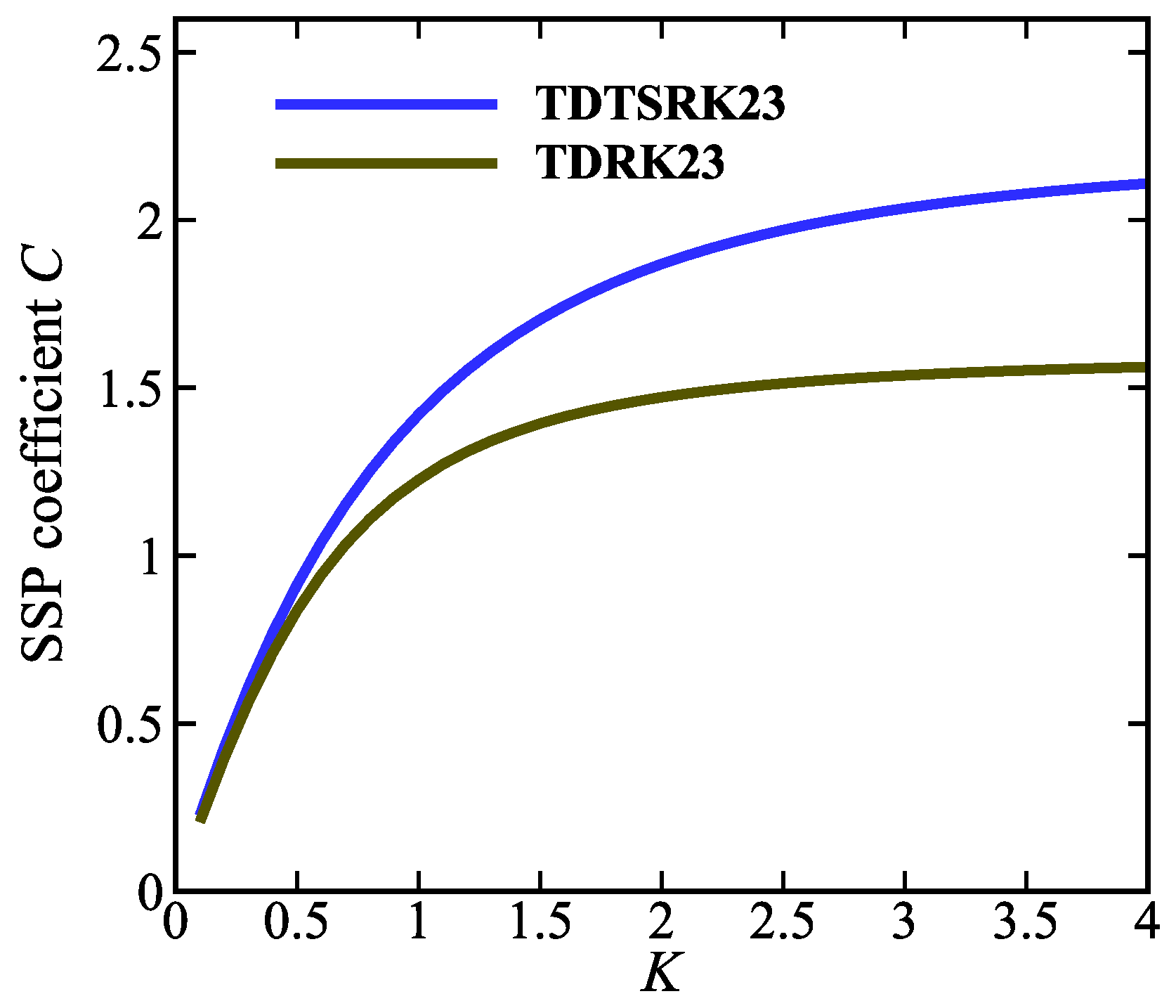
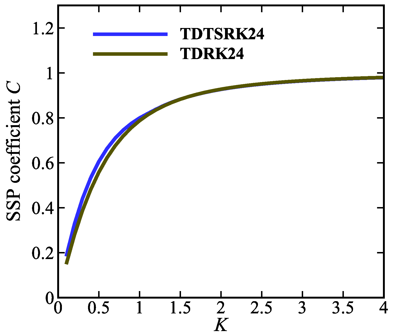
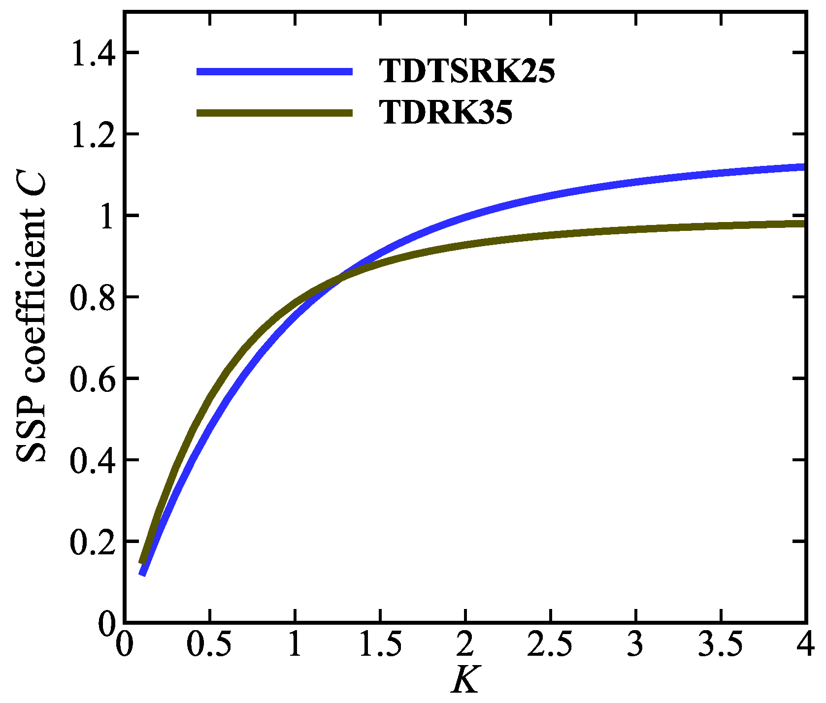
3.3. Optimal SSP TDTSRK Methods

We formulated the SSP condition for TDTSRK methods in Section 3.2, and give coefficients for some high-order TDTSRK methods in Section 2.3. In this section, we will search the optimal SSP coefficients $\mathcal{C}$ and corresponding coefficients for TDTSRK methods.

First, due to the assumed limitation for the SSP condition for TDTSRK methods, the values of $w_i$ and ${\widehat{w}}_i$ for TDTSRK methods should be constrained in a specific range. The TDTSRK23 method and TDTSRK24 method have many parameters to determine, making it difficult to find the optimal SSP coefficients $\mathcal{C}$. We can specify the values of some parameters and choose the range of other parameters. For the six parameters of the TDTSRK23 method, the values of $w_1$, $w_2$, ${\widehat{w}}_1$, and ${\widehat{w}}_1$ are given, the ranges of $v_2$ and $a_{21}$ are determined. For the four-parameter TDTSRK24 method, the values of $w_2$, ${\widehat{w}}_1$, and $v_1$ are given, and the range of $a_{21}$ is determined. For the one-parameter TDTSRK24 method, the range of $a_{21}$ is determined. Then, we have the range of $w_i$ and ${\widehat{w}}_i$ for TDTSRK methods, which are displayed in

Table 2. The values and range of parameters for the different TDTSRK methods.

	TDTSRK23	TDTSRK24	TDTSRK25
Values of parameters	$w_1=0.0$ $w_2=0.1$ ${\widehat{w}}_1=0.0$ ${\widehat{w}}_2=0.0$	$w_2=-0.1$ ${\widehat{w}}_2=0.0$ $v_1=1.0$	$—$
Range of parameters	$0.0<v_2<1.0$ $0.0<a_{21}<1.0$	$0.0<a_{21}<1.0$	$0.758\le a_{21}\le 0.765$
Range of $w_i$ and ${\widehat{w}}_i$	$—$	$w_1=0.0$ $|{\widehat{w}}_1| < 0.05$	$|w_1| < 0.06,$$w_2=0.0$ $|{\widehat{w}}_1| < 0.15,$$|{\widehat{w}}_2| < 0.15$

.

By these given parameters, the six-parameter into the two-parameter ($v_2$, $a_{21}$) of the TDTSRK23 method, the four-parameter into the one-parameter ($a_{21}$) of TDTSRK24 method, and the range of these parameters for TDTSRK methods have been determined. The optimal SSP coefficient $\mathcal{C}$ is also dependent on the value K. Figure 3, Figure 4 and Figure 5 present the optimal SSP coefficient $\mathcal{C}$ of TDTSRK methods for the range $0.1\le K\le 4$, and compare it with the SSP coefficient of the TDRK schemes [27]. The parameters for TDTSRK methods corresponding to the optimal SSP coefficient $\mathcal{C}$ for each value K are given in

Table 3. The optimal SSP coefficient $\mathcal{C}$ of the TDTSRK and TDRK methods for each K and the corresponding parameters $a_{21}$, $v_2$ for the TDTSRK and TDRK methods.

K	TDTSRK23			TDRK23	TDTSRK24		TDRK24	TDTSRK25		TDRK35
	${\mathit{a}}_{\mathbf{21}}$	${\mathit{v}}_{\mathbf{2}}$	$\mathcal{C}$	$\mathcal{C}$	${\mathit{a}}_{\mathbf{21}}$	$\mathcal{C}$	$\mathcal{C}$	${\mathit{a}}_{\mathbf{21}}$	$\mathcal{C}$	${\mathit{a}}_{\mathbf{21}}$	$\mathcal{C}$
0.1	0.583	0.354	0.226	0.206	0.579	0.184	0.149	0.758	0.116	0.795	0.145
0.2	0.572	0.354	0.429	0.396	0.532	0.327	0.278	0.758	0.222	0.784	0.272
0.3	0.563	0.363	0.610	0.564	0.510	0.441	0.388	0.758	0.317	0.775	0.381
0.4	0.555	0.371	0.771	0.711	0.495	0.533	0.481	0.758	0.402	0.767	0.474
0.5	0.547	0.377	0.914	0.837	0.484	0.606	0.558	0.758	0.478	0.761	0.552
0.6	0.540	0.383	1.041	0.944	0.475	0.663	0.622	0.765	0.547	0.755	0.617
$\sqrt{2}/2$	0.532	0.389	1.161	1.040	0.468	0.712	0.679	0.765	0.635	0.750	0.675
0.8	0.527	0.393	1.253	1.110	0.464	0.746	0.720	0.765	0.662	0.747	0.716
1.0	0.515	0.401	1.420	1.226	0.457	0.800	0.787	0.765	0.754	0.741	0.785
1.5	0.494	0.416	1.704	1.394	0.954	0.883	0.883	0.765	0.907	0.733	0.882
2.0	0.481	0.426	1.869	1.472	0.970	0.927	0.928	0.765	0.995	0.728	0.927
3.0	0.467	0.437	2.035	1.537	0.985	0.964	0.965	0.765	1.082	0.277	0.965
4.0	0.460	0.442	2.109	1.562	0.990	0.979	0.980	0.765	1.119	0.270	0.980

. For $K={\displaystyle \frac{\sqrt{2}}{2}}$, the optimal parameters matrices of TDMSRK schemes are shown in Appendix B.

4. Numerical Experiments

In this section, several standard benchmark cases are conducted to evaluate the SSP property and order of accuracy for the TDTSRK methods. We compare the TDTSRK methods with TDRK methods and RK methods, which are given below:

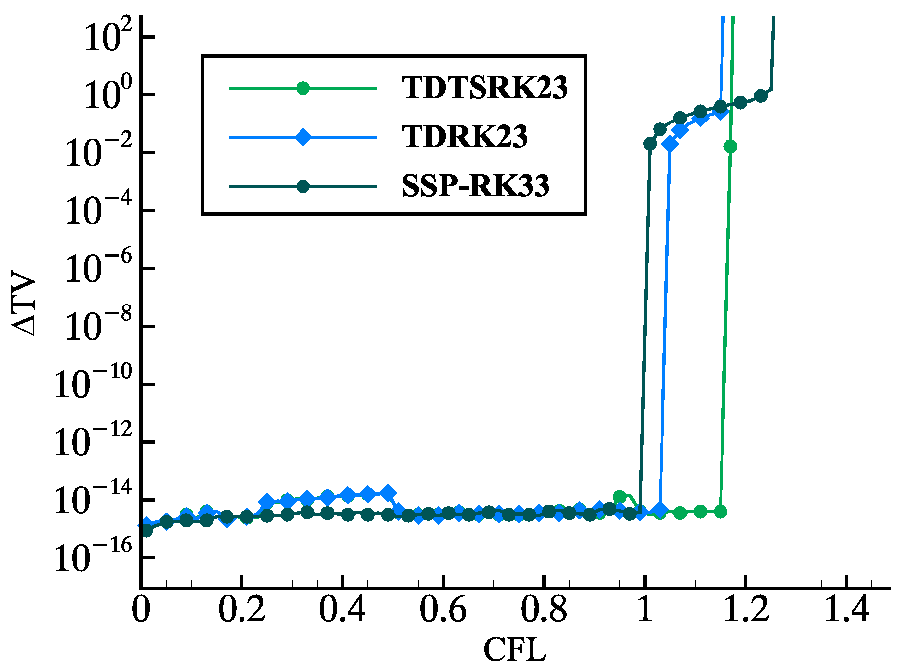
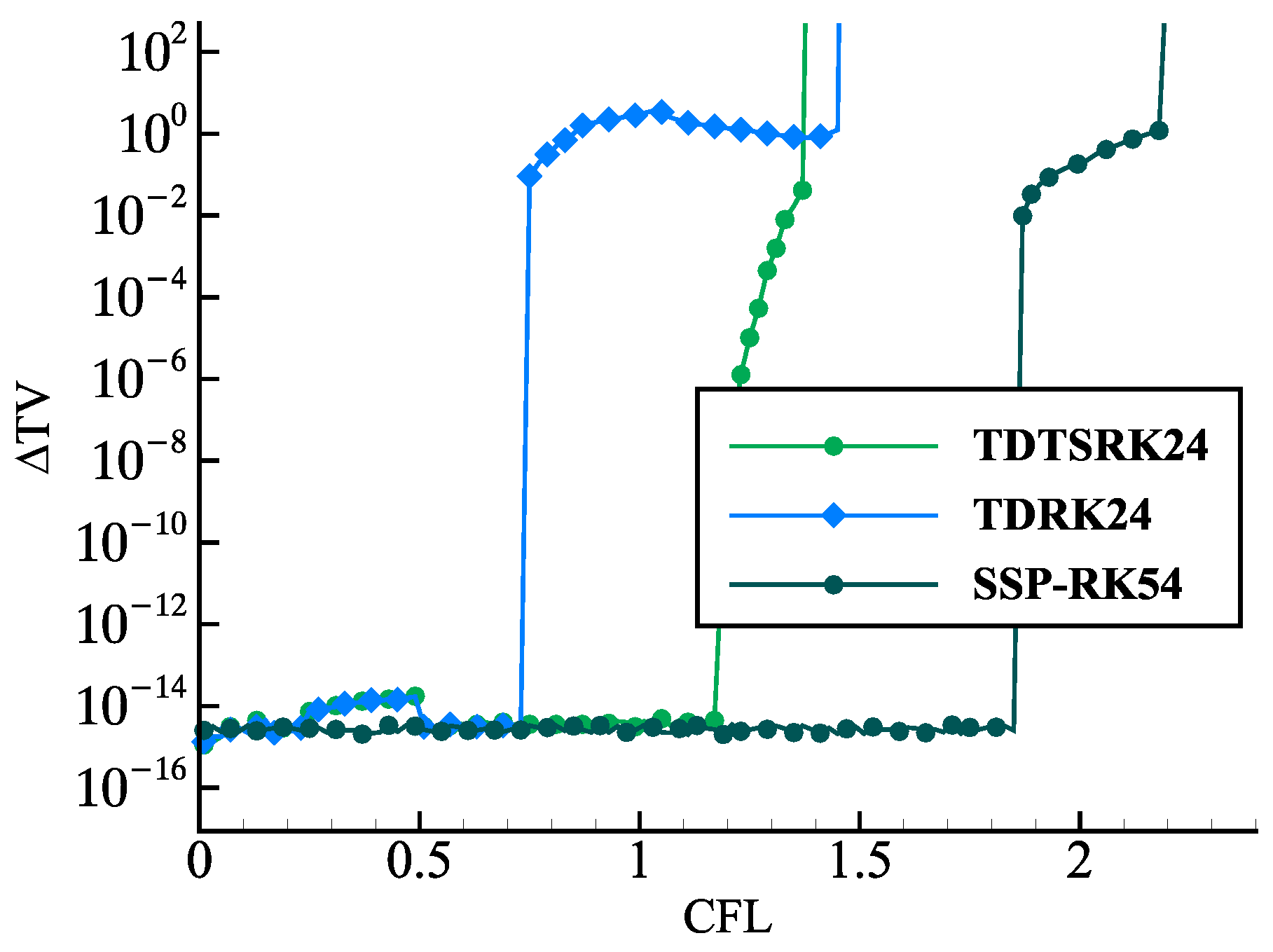
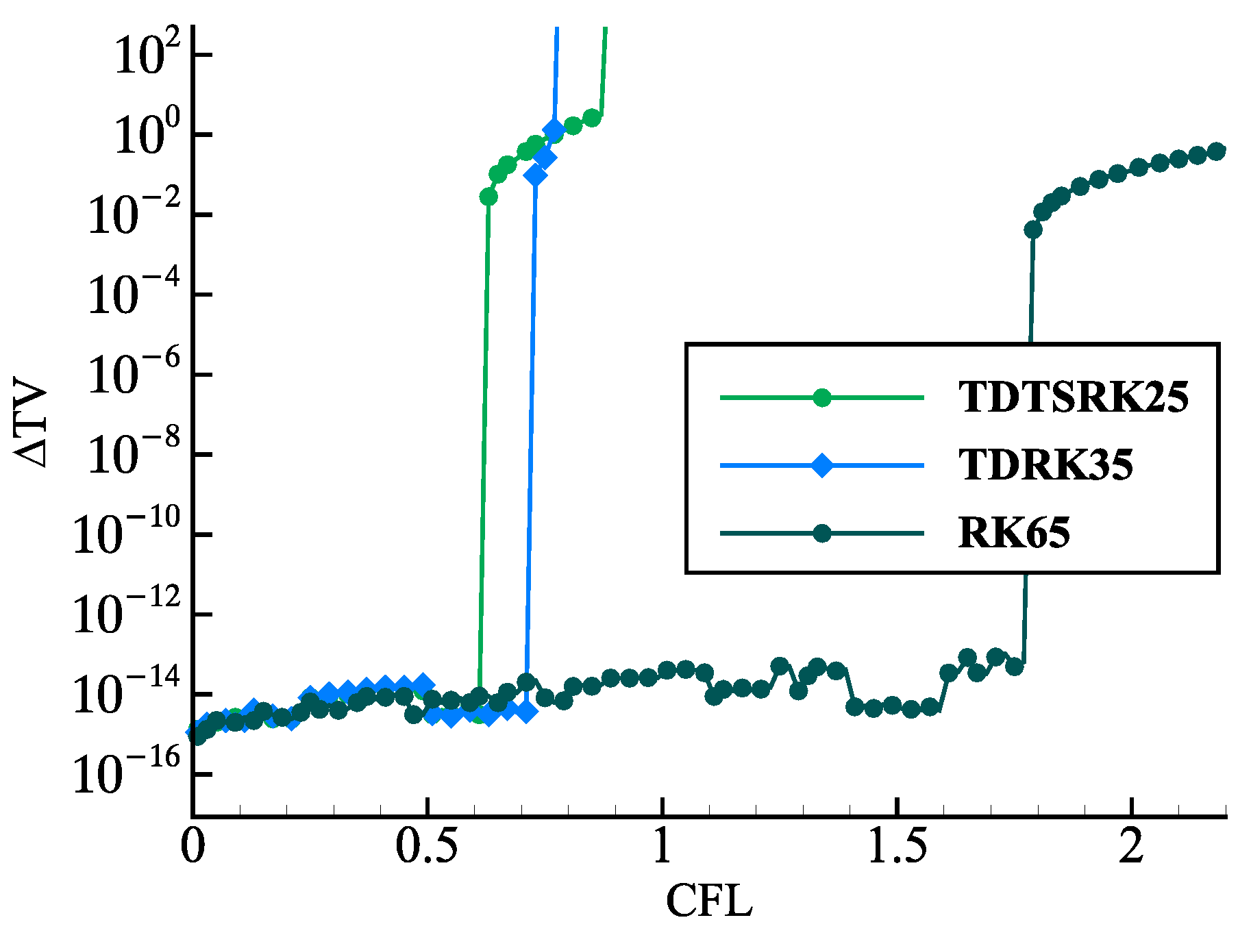
• TDTSRK23, TDTSRK24, TDTSRK25: the two-stage third-order, two-stage fourth-order, and two-stage fifth-order TDTSRK methods are shown in Appendix B.
• TDRK23, TDRK24, TDRK35: the two-stage third-order, two-stage fourth-order, and three-stage fifth-order TDRK methods are quoted from [27].
• SSP-RK33: the three-stage third-order SSP-RK method is the most popular explicit time scheme in Shu and Stanley [3].
• SSP-RK54: the five-stage fourth-order SSP-RK method is presented by Spiteri [33].
• RK65: the classical six-stage fifth-order RK method is given in Butcher [34].

We take these numerical verification on Equation (1), and rewrite the equation as

$$u_t+f{\left(u\right)}_x=0.$$

(41)

In Section 4.1 and Section 4.2, we focus on investigating the SSP properties of the proposed methods in terms of the total variation (TV). We adopt the maximum TV property to measure the SSP condition, i.e., by comparing the rise of TV to that of the initial solution, defined by

$$\Delta \mathrm{TV}=\underset{0\le n\le N-1}{\max }\left(\parallel u^{n+1}{\parallel }_{\mathrm{TV}}-{\parallel u^0\parallel }_{\mathrm{TV}}\right).$$

(42)

The SSP standard is defined by a maximal increase of $1\times {10}^{-10}$. For the linear advection, we calculate the first derivative and second derivative by Equation (37). For the nonlinear Burgers’ equation, we have the flux $f\left(u\right)={\displaystyle \frac{u^2}{2}}$ and obtain

$$u_t=-f{\left(u\right)}_x,u_{tt}=-{\left(f{\left(u\right)}_t\right)}_x=-{\left(f_u\left(u\right)u_t\right)}_x.$$

(43)

In Section 4.3 and Section 4.4, we mainly test the order of accuracy for the TDTSRK methods. To show the time accuracy directly, we use the eighth-order up-wind scheme to compute the first derivatives and use the eighth-order center scheme to compute second derivatives. For the linear advection, these schemes are given by

$$\begin{array}{cc}\hfill F\left(u_i^n\right)=& (3u_{i+5}^n-30u_{i+4}^n+140u_{i+3}^n-420u_{i+2}^n+1050u_{i+1}^n-378u_i^n\hfill \\ \hfill & -420u_{i-1}^n+60u_{i-2}^n-5u_{i-3}^n)/(840\Delta x),\hfill \\ \hfill G\left(u_i^n\right)=& (-63u_{i+4}^n+896u_{i+3}^n-7056u_{i+2}^n+56448u_{i+1}^n-100450u_i^n\hfill \\ \hfill & +56448u_{i-1}^n-7056u_{i-2}^n+896u_{i-3}^n-63u_{i-4}^n)/(35280\Delta x^2).\hfill \end{array}$$

(44)

For the nonlinear Burgers’ equation, these schemes are defined as

$$\begin{array}{cc}\hfill F\left(u_i^n\right)=& (5f\left(u_{i+3}^n\right)-60f\left(u_{i+2}^n\right)+420f\left(u_{i+1}^n\right)+378f\left(u_i^n\right)-1050f\left(u_{i-1}^n\right)\hfill \\ \hfill & +420f\left(u_{i-2}^n\right)-140f\left(u_{i-3}^n\right)+30f\left(u_{i-4}^n\right)-3f\left(u_{i-5}^n\right))/(840\Delta x),\hfill \\ \hfill G\left(u_i^n\right)=& (-3f{\left(u_{i+4}^n\right)}_t+32f{\left(u_{i+3}^n\right)}_t-168f{\left(u_{i+2}^n\right)}_t+672f{\left(u_{i+1}^n\right)}_t\hfill \\ \hfill & -672f{\left(u_{i-1}^n\right)}_t+168f{\left(u_{i-2}^n\right)}_t-32f{\left(u_{i-3}^n\right)}_t+3f{\left(u_{i-4}^n\right)}_t)/(840\Delta x).\hfill \end{array}$$

(45)

We use the RK65 method for TDTSRK methods in startup procedures to test the order of accuracy. For other cases, we take the same order accuracy TDRK methods in startup procedures. In our simulations, we adopt periodic boundary conditions for computation.

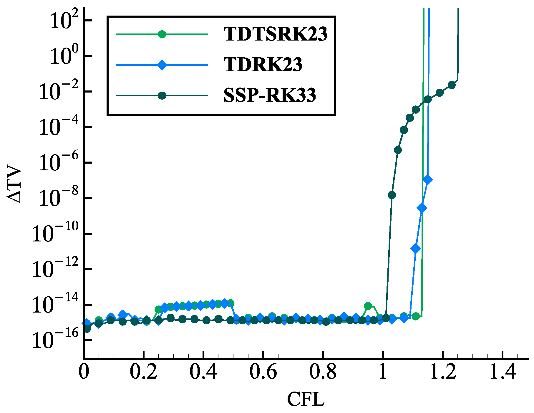
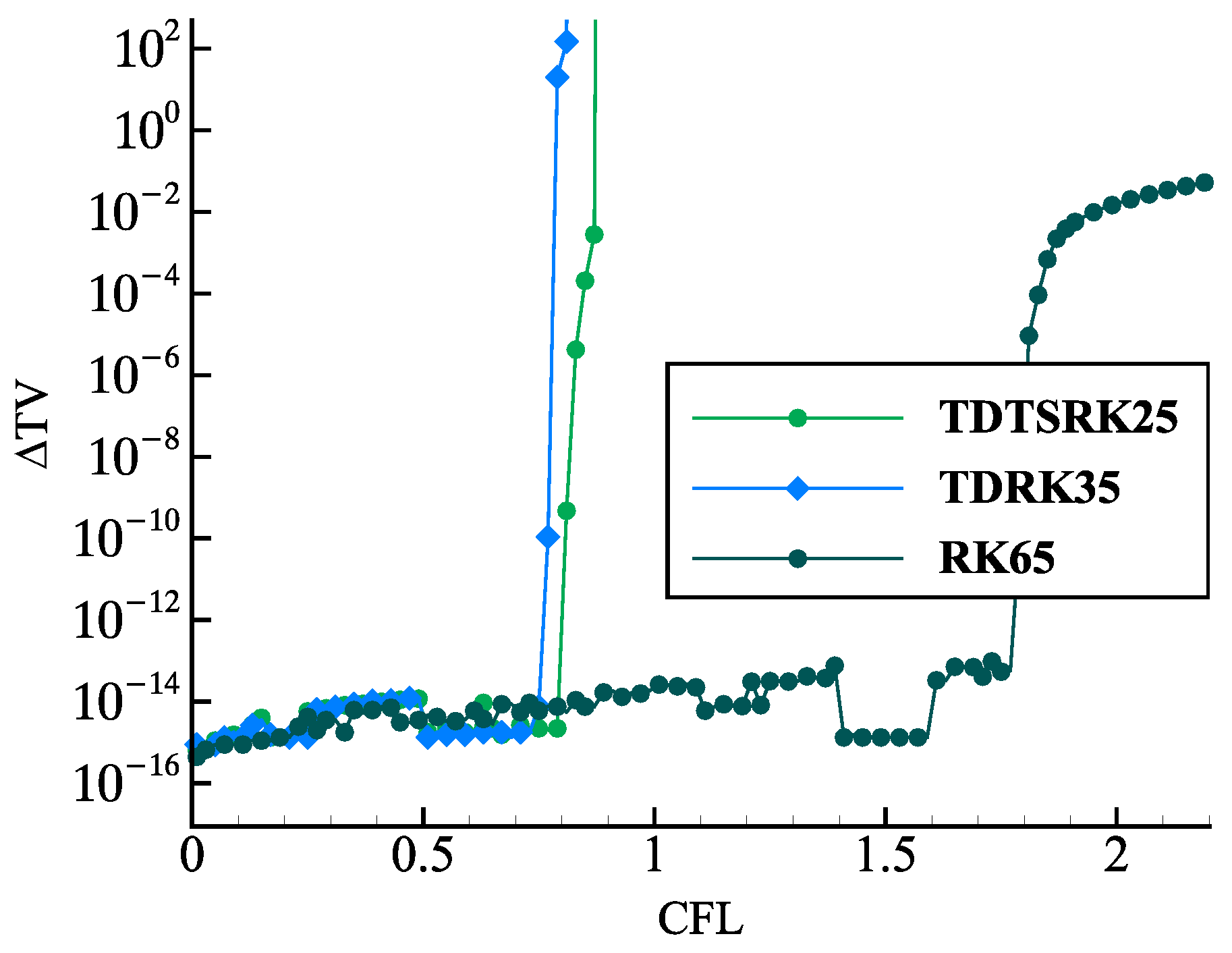
4.1. SSP Properties of the TDTSRK Methods on the Linear Advection

In this example, we consider the linear advection

$$u_t-u_x=0,$$

(46)

and calculate the first derivative and second derivative by Equation (37). For initial conditions, a step function is used as

$$u_0\left(x\right)=\left\{\begin{array}{c}1\mathrm{if}-{\displaystyle \frac{1}{2}}\le x\le {\displaystyle \frac{1}{2}},\hfill \\ 0\mathrm{otherwise}.\hfill \end{array}\right.$$

(47)

We use a fixed grid of size $\Delta x={\displaystyle \frac{1}{1600}}$ in the spatial domain $x\in [-2,2]$ and the time step size $\Delta t=\mathrm{CFL}·\Delta x/{\parallel u\parallel }_{\max }$, where ${\parallel u\parallel }_{\max }=1.0$. We vary $0.02\le \mathrm{CFL}\le 2.5$ and advance each scheme forward by $N=500$ timesteps.

This example is tested using the TDTSRK methods, TDRK methods, and RK methods. The parameters we use for TDTSRK methods correspond to $K={\displaystyle \frac{\sqrt{2}}{2}}$ in Table 3. Figure 6, Figure 7 and Figure 8 show that the rise in total variation vs. the Courant-Friedrichs-Lewy (CFL) for different order accuracy methods. We clearly see that once the CFL value passes a certain limit defined as the observed SSP coefficient ${\mathcal{C}}^{\ast }$, there is a sharp jump in the TV of the solution. In

Table 4. Comparison of the SSP coefficient and effective SSP coefficient for different temporal discretization methods in the theoretical and observed result.

	TDTS	TD	SSP-	TDTS	TD	SSP-	TDTS	TD	RK65
	RK23	RK23	RK33	RK24	RK24	RK54	RK25	RK35
$\mathcal{C}$	1.161	1.040	1.000	0.712	0.679	1.508	0.635	0.675	−
${\mathcal{C}}_{\mathrm{eff}}$	0.581	0.520	0.333	0.356	0.340	0.302	0.318	0.225	−
$\gamma$	111.6%	100%	64.1%	104.9%	100%	88.8%	141.1%	100%	−
${\mathcal{C}}^{\ast }$	1.168	1.040	1.000	1.189	0.732	1.861	0.622	0.714	1.777
${\mathcal{C}}_{\mathrm{eff}}^{\ast }$	0.585	0.520	0.333	0.595	0.366	0.372	0.311	0.238	0.296
$\gamma$	112.3%	100%	64.1%	162.4%	100%	101.7%	130.7%	100%	124.4%

, we compare the predicted theoretical SSP coefficient $\mathcal{C}$ with those observed in numerical examples, and we define the effective SSP coefficient ${\mathcal{C}}_{\mathrm{eff}}=\mathcal{C}/s$ to compare these schemes with different numbers of stages s. To see the comparison for same order accuracy methods conveniently, we set $\gamma$ to represent the ratio of the effective SSP coefficient ${\mathcal{C}}_{\mathrm{eff}}$. The TDTSRK methods have the largest effective SSP coefficient ${\mathcal{C}}_{\mathrm{eff}}$ in the same order of accuracy.

4.2. SSP Properties of the TDTSRK Methods on the Burgers’ Equation

We consider the Burgers’ equation

$$u_t+{\left({\displaystyle \frac{u^2}{2}}\right)}_x=0,$$

(48)

and repeat the simulation above with all the same conditions and parameters in Section 4.1. In Figure 9, Figure 10 and Figure 11, and

Table 5. Comparison of the SSP coefficient ${\mathcal{C}}^{\ast }$ and effective SSP coefficient ${\mathcal{C}}_{\mathrm{eff}}^{\ast }$ for different temporal discretization methods on the Burgers’ equation.

	TDTS	TD	SSP-	TDTS	TD	SSP-	TDTS	TD	RK65
	RK23	RK23	RK33	RK24	RK24	RK54	RK25	RK35
${\mathcal{C}}^{\ast }$	1.143	1.117	1.021	1.134	0.849	1.886	0.807	0.769	1.789
${\mathcal{C}}_{\mathrm{eff}}^{\ast }$	0.572	0.559	0.340	0.567	0.425	0.377	0.404	0.256	0.298
$\gamma$	102.3%	100%	60.9%	133.6%	100%	88.9%	157.4%	100%	116.3%

, we observe a similar behavior as the linear advection example. By comparing the TDTSRK methods with TDRK methods and RK methods, it is clearly shown that the TDTSRK methods have the largest effective SSP coefficient ${\mathcal{C}}_{\mathrm{eff}}$ in the same order of accuracy.

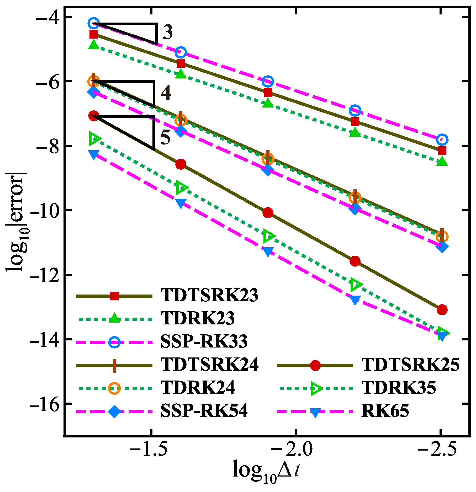
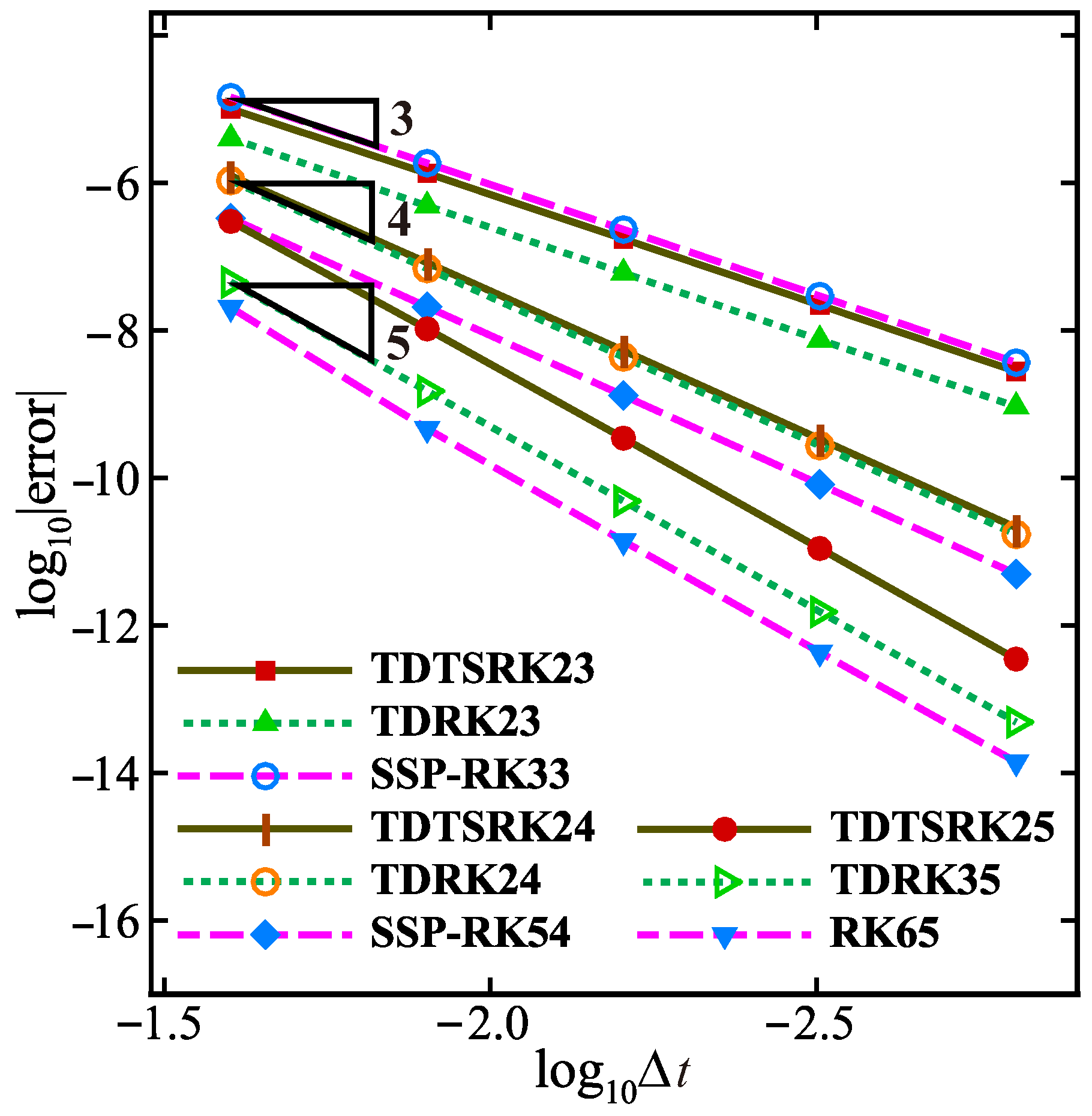
4.3. Order Accuracy of the TDTSRK Methods on the Linear Advection

We test the order accuracy of temporal methods on the linear advection Equation (46). The exact solution is $u(x,t)=0.5sin\left(\pi \right(x-t\left)\right)+0.5$ in domain $x\in [0,2]$, and the parameters of the TDTSRK methods are the same as in Section 4.1. The time step size $\Delta t=\mathrm{CFL}·\Delta x/{\parallel u\parallel }_{\max }$, where $\mathrm{CFL}=0.5$ and ${\parallel u\parallel }_{\max }=1.0$. In

Table 6. The order accuracy for third-order accuracy methods on the linear advection.

Grid	TDTSRK23		TDRK23		SSP-RK33
	${\mathit{L}}_{\infty }$ Error	Order	${\mathit{L}}_{\infty }$ Error	Order	${\mathit{L}}_{\infty }$ Error	Order
40	$2.86\times {10}^{-05}$	$—$	$1.25\times {10}^{-05}$	$—$	$6.33\times {10}^{-05}$	$—$
80	$3.61\times {10}^{-06}$	2.99	$1.56\times {10}^{-06}$	3.00	$7.92\times {10}^{-06}$	3.00
160	$4.53\times {10}^{-07}$	2.99	$1.95\times {10}^{-07}$	3.00	$9.91\times {10}^{-07}$	3.00
320	$5.67\times {10}^{-08}$	3.00	$2.44\times {10}^{-08}$	3.00	$1.24\times {10}^{-07}$	3.00
640	$7.09\times {10}^{-09}$	3.00	$3.05\times {10}^{-09}$	3.00	$1.55\times {10}^{-08}$	3.00

,

Table 7. The order accuracy for fourth-order accuracy methods on the linear advection.

Grid	TDTSRK24		TDRK24		SSP-RK54
	${\mathit{L}}_{\infty }$ Error	Order	${\mathit{L}}_{\infty }$ Error	Order	${\mathit{L}}_{\infty }$ Error	Order
40	$1.14\times {10}^{-06}$	$—$	$9.92\times {10}^{-07}$	$—$	$4.58\times {10}^{-07}$	$—$
80	$7.16\times {10}^{-08}$	3.99	$6.22\times {10}^{-08}$	3.99	$2.88\times {10}^{-08}$	3.99
160	$4.49\times {10}^{-09}$	3.99	$3.89\times {10}^{-09}$	4.00	$1.80\times {10}^{-09}$	4.00
320	$2.81\times {10}^{-10}$	4.00	$2.43\times {10}^{-10}$	4.00	$1.13\times {10}^{-10}$	4.00
640	$1.76\times {10}^{-11}$	4.00	$1.52\times {10}^{-11}$	4.00	$7.66\times {10}^{-12}$	3.88

and

Table 8. The order accuracy for fifth-order accuracy methods on the linear advection.

Grid	TDTSRK25		TDRK35		RK65
	${\mathit{L}}_{\infty }$ Error	Order	${\mathit{L}}_{\infty }$ Error	Order	${\mathit{L}}_{\infty }$ Error	Order
40	$8.49\times {10}^{-08}$	$—$	$1.68\times {10}^{-08}$	$—$	$5.72\times {10}^{-09}$	$—$
80	$2.69\times {10}^{-09}$	4.98	$5.11\times {10}^{-10}$	5.04	$1.78\times {10}^{-10}$	5.01
160	$8.44\times {10}^{-11}$	4.99	$1.59\times {10}^{-11}$	5.00	$5.57\times {10}^{-12}$	4.99
320	$2.64\times {10}^{-12}$	5.00	$4.98\times {10}^{-13}$	5.00	$1.76\times {10}^{-13}$	4.98
640	$8.26\times {10}^{-14}$	5.00	$1.55\times {10}^{-14}$	5.00	$1.33\times {10}^{-14}$	3.72

, we show the $L_{\infty }$ error of these time-discretization methods for different order accuracy at final time $T_f=2.0$. The $L_{\infty }$ is equal to the maximum absolute value of the errors at all grid points, $L_{\infty }=\max |\Delta u_i^n|$. In Figure 12, we observe that the TDTSRK methods can achieve the expected order of accuracy, the absolute errors of TDTSRK schemes are close to those of TDRK schemes, and their absolute errors are larger than those of RK schemes except in third-order accuracy.

4.4. Order Accuracy of the TDTSRK Methods on the Burgers’ Equation

We calculate the order of accuracy for temporal methods on the Burgers’ equation Equation (48). In this example, the initial condition and other simulation conditions are same as in Section 4.3. To show the temporal order of accuracy clearly, we take $\mathrm{CFL}=0.8$ and final time $T_f=0.2$. In

Table 9. The order accuracy for third-order accuracy methods on the Burgers’ equation.

Grid	TDTSRK23		TDRK23		SSP-RK33
	${\mathit{L}}_{\infty }$ Error	Order	${\mathit{L}}_{\infty }$ Error	Order	${\mathit{L}}_{\infty }$ Error	Order
80	$1.00\times {10}^{-05}$	$—$	$4.02\times {10}^{-06}$	$—$	$1.45\times {10}^{-05}$	$—$
160	$1.35\times {10}^{-06}$	2.90	$4.87\times {10}^{-07}$	3.05	$1.85\times {10}^{-06}$	2.97
320	$1.74\times {10}^{-07}$	2.95	$6.00\times {10}^{-08}$	3.02	$2.33\times {10}^{-07}$	2.99
640	$2.20\times {10}^{-08}$	2.98	$7.45\times {10}^{-09}$	3.01	$2.92\times {10}^{-08}$	3.00
1280	$2.77\times {10}^{-09}$	2.99	$9.28\times {10}^{-10}$	3.00	$3.65\times {10}^{-09}$	3.00

,

Table 10. The order accuracy for fourth-order accuracy methods on the Burgers’ equation.

Grid	TDTSRK24		TDRK24		SSP-RK54
	${\mathit{L}}_{\infty }$ Error	Order	${\mathit{L}}_{\infty }$ Error	Order	${\mathit{L}}_{\infty }$ Error	Order
80	$1.25\times {10}^{-06}$	$—$	$1.07\times {10}^{-06}$	$—$	$3.31\times {10}^{-07}$	$—$
160	$8.28\times {10}^{-08}$	3.91	$6.89\times {10}^{-08}$	3.96	$2.08\times {10}^{-08}$	3.99
320	$5.32\times {10}^{-09}$	3.96	$4.36\times {10}^{-09}$	3.98	$1.31\times {10}^{-09}$	3.99
640	$3.37\times {10}^{-10}$	3.98	$2.73\times {10}^{-10}$	3.99	$8.17\times {10}^{-11}$	4.00
1280	$2.12\times {10}^{-11}$	3.99	$1.71\times {10}^{-11}$	4.00	$4.96\times {10}^{-12}$	4.04

and

Table 11. The order accuracy for fifth-order accuracy methods on the Burgers’ equation.

Grid	TDTSRK25		TDRK35		RK65
	${\mathit{L}}_{\infty }$ Error	Order	${\mathit{L}}_{\infty }$ Error	Order	${\mathit{L}}_{\infty }$ Error	Order
80	$3.00\times {10}^{-07}$	$—$	$4.50\times {10}^{-08}$	$—$	$2.04\times {10}^{-08}$	$—$
160	$1.05\times {10}^{-08}$	4.84	$1.51\times {10}^{-09}$	4.90	$4.65\times {10}^{-10}$	5.45
320	$3.45\times {10}^{-10}$	4.92	$4.85\times {10}^{-11}$	4.96	$1.39\times {10}^{-11}$	5.06
640	$1.11\times {10}^{-11}$	4.97	$1.53\times {10}^{-12}$	4.98	$4.32\times {10}^{-13}$	5.01
1280	$3.49\times {10}^{-13}$	4.98	$4.88\times {10}^{-14}$	4.97	$1.41\times {10}^{-14}$	4.94

and Figure 13, the numerical result show that the TDTSRK methods can achieve the designed order of accuracy, the absolute errors of TDTSRK schemes have the same behavior on the linear advection.

4.5. Efficiency for TDMSRK Schemes

We assess the efficiency of different schemes on the two-dimensional (2D) Euler equation, the conservation form of the 2D Euler equation can be obtained as

$${\displaystyle \frac{\partial \mathbf{W}}{\partial t}}+{\displaystyle \frac{\partial {\mathbf{H}}_1}{\partial x}}+{\displaystyle \frac{\partial {\mathbf{H}}_2}{\partial y}}=0,$$

(49)

where

$$\mathbf{W}=\left[\begin{array}{c}\rho \\ \rho u\\ \rho v\\ E\end{array}\right],{\mathbf{H}}_1=\left[\begin{array}{c}\rho u\\ \rho u^2+p\\ \rho uv\\ (E+p)u\end{array}\right],{\mathbf{H}}_2=\left[\begin{array}{c}\rho v\\ \rho uv\\ \rho v^2+p\\ (E+p)v\end{array}\right],$$

(50)

and u, v are the velocity in the x direction and y direction, p is the pressure, $\rho$ is the density, the energy E is defined by $E={\displaystyle \frac{p}{\gamma -1}}+{\displaystyle \frac{1}{2}}\rho (u^2+v^2)$. The $\gamma$ is the ratio of specific heats and we take $\gamma =1.4$. The seventh-order WENO7Z method [35] and sixth-order center method are utilized for spatial schemes to calculate the first derivative and second derivative, the details of the spatial schemes are given in [15].

The isotropic vortex propagation problem is utilized to test the TDTSRK schemes on the 2D Euler equations. The mean flow is $(\rho ,u,v,p)=(1,1,1,1)$ in domain [−5, 5] × [−5, 5]. A small vortex is obtained through a perturbation on the mean flow with the velocity $(u,v)$, temperature $T=p/\rho$, and entropy $S=p/{\rho }^{\gamma }$, the perturbation is given by

$$(\delta u,\delta v)={\displaystyle \frac{\varphi }{2\pi }}{e}^{{\displaystyle \frac{(1-r^2)}{2}}}(-\delta y,\delta x),\delta T=-{\displaystyle \frac{(\gamma -1){\varphi }^2}{8\gamma {\pi }^2}}{e}^{1-r^2},\delta S=0,$$

(51)

where $r^2=x^2+y^2$, and the vortex strength $\varphi =5$. The time-step is $\Delta t={\mathrm{CFL}/\left(\right(\parallel u\parallel +c)}_{\max }/\Delta x+{(\parallel v\parallel +c)}_{\max }/\Delta y)$, we choose $\mathrm{CFL}=1.0$ and ${(\parallel u\parallel +c)}_{\max }={(\parallel v\parallel +c)}_{\max }=3.0$ according to the initial condition. The mesh number is 150 × 150 and the density $\rho$ distributions is shown in Figure 14 at final time $T_f=10.0$. In

Table 12. The total CPU time cost of different temporal schemes on the 2D Euler equation.

	TDTS	TD	SSP-	TDTS	TD	SSP-	TDTS	TD	RK65
	RK23	RK23	RK33	RK24	RK24	RK54	RK25	RK35
Stage s	2	2	3	2	2	5	2	3	6
CPU Time	256.3	254.7	327.5	256.8	254.9	548.2	256.9	386.4	655.1
Ratio $\phi$	2.35	2.33	3.00	2.35	2.33	5.02	2.35	3.54	6.00

, we show the total CPU time cost of different temporal schemes on the 2D Euler equation. We define the CPU time ratio $\phi$ with respect to one-sixth of the ${\mathrm{RK}}_{33}$ method. The numerical result is shown that the ratio is roughly 1.0 for each stage of RK and TSRK methods, the ratio is roughly 1.17 for each stage of TDTSRK and TDRK methods. The CPU time cost of TDTSRK methods is equal to that of TDRK methods in the third-order and fourth-order accuracy, but the TDTSRK methods allow for a larger time step size than the TDRK methods. Consequently, the TDTSRK methods are more efficient than the TDRK and RK methods in the same order of accuracy.

5. Conclusions

We formulate the order conditions for TDTSRK methods using Albrecht’s approach, demonstrating that these conditions are simpler and less numerous than the order conditions provided by the rooted trees theory, particularly for high-order conditions. We also present some two-stage TDTSRK methods up to the fifth order and verify that these methods satisfy the designed order conditions. Based on the construction of TDTSRK methods, we propose the SSP theory for the TDTSRK methods under some assumptions. Despite these constraints, the optimal SSP coefficient derived from the SSP theory closely aligns with the result observed in the numerical example, thereby validating the reasonableness of the SSP theory for TDTSRK methods. Furthermore, we evaluate the numerical stability of TDTSRK methods and compare them with TDRK and RK methods, which indicates that TDTSRK methods have the largest effective SSP coefficient among these methods. Numerical results demonstrate that the TDTSRK methods are highly efficient in solving the partial differential equation.

References

1. Jiang, G.-S.; Shu, C.-W. Efficient implementation of weighted ENO schemes. J. Comput. Phys. 1996, 126, 202–228. [Google Scholar] [CrossRef]
2. Cockburn, B.; Shu, C.-W. Runge-Kutta discontinuous galerkin methods for convection-dominated problems. J. Sci. Comput. 2001, 16, 173–261. [Google Scholar] [CrossRef]
3. Shu, C.-W.; Osher, S. Efficient implementation of essentially non-oscillatory shock-capturing methods. J. Comput. Phys. 1988, 77, 439–471. [Google Scholar] [CrossRef]
4. Askar, A.H.; Nagy, Á.; Barna, I.F.; Kovács, E. Analytical and Numerical Results for the Diffusion-Reaction Equation When the Reaction Coefficient Depends on Simultaneously the Space and Time Coordinates. Computation 2023, 11, 127. [Google Scholar] [CrossRef]
5. Khayrullaev, H.; Omle, I.; Kovács, E. Systematic Investigation of the Explicit, Dynamically Consistent Methods for Fisher’s Equation. Computation 2024, 12, 49. [Google Scholar] [CrossRef]
6. Ding, H.; Zhang, Y. A new difference scheme with high accuracy and absolute stability for solving convection-diffusion equations. J. Comput. Appl. Math. 2009, 230, 600–606. [Google Scholar] [CrossRef]
7. Gottlieb, S.; Ketcheson, D.I.; Shu, C.-W. Strong Stability Preserving Runge-Kutta and Multistep Time Discretizations; World Scientific: Singapore, 2011. [Google Scholar]
8. Qin, X.; Yu, J.; Yan, C. Derivation of Three-Derivative Two-Step Runge–Kutta Methods. Mathematics 2024, 12, 711. [Google Scholar] [CrossRef]
9. Qin, X.; Yu, J.; Jiang, Z.; Huang, L.; Yan, C. Explicit strong stability preserving second derivative multistep methods for the Euler and Navier-Stokes equations. Comput. Fluids 2024, 268, 106089. [Google Scholar] [CrossRef]
10. Afsaneh, M.; Jeremy, C.; Raffaele, D.; Jochen, S. Jacobian-free explicit multiderivative general linear methods for hyperbolic conservation laws. Numer. Algorithms 2024, 1572–9265. [Google Scholar]
11. Kovalnogov, V.N.; Fedorov, R.V.; Karpukhina, T.V.; Simos, T.E.; Tsitouras, C. On Reusing the Stages of a Rejected Runge-Kutta Step. Mathematics 2023, 11, 2589. [Google Scholar] [CrossRef]
12. Gottlieb, S.; Ketcheson, D.I. Time discretization techniques. In Handbook of Numerical Analysis; Elsevier: Amsterdam, The Netherlands, 2016; Volume 17, pp. 549–583. [Google Scholar]
13. Gottlieb, S.; Ketcheson, D.I.; Shu, C.-W. High order strong stability preserving time discretizations. J. Sci. Comput. 2009, 38, 251–289. [Google Scholar] [CrossRef]
14. Seal, D.C.; Güçlü, Y.; Christlieb, A.J. High-order multiderivative time integrators for hyperbolic conservation laws. J. Sci. Comput. 2014, 60, 101–140. [Google Scholar] [CrossRef]
15. Qin, X.; Jiang, Z.; Yu, J.; Huang, L.; Yan, C. Strong stability-preserving three-derivative Runge–Kutta methods. Comput. Appl. Math. 2023, 42, 171. [Google Scholar] [CrossRef]
16. Butcher, J.C. An algebraic theory of integration methods. Math. Comput. 1972, 26, 79–106. [Google Scholar] [CrossRef]
17. Butcher, J.C. Trees and numerical methods for ordinary differential equations. Numer. Algorithms 2010, 53, 153–170. [Google Scholar] [CrossRef]
18. Albrecht, P. The Runge-Kutta theory in a nutshell. SIAM J. Numer. Anal. 1996, 33, 1712–1735. [Google Scholar] [CrossRef]
19. Butcher, J.C.; Tracogna, S. Order conditions for two-step Runge-Kutta methods. Appl. Numer. Math. 1997, 24, 351–364. [Google Scholar] [CrossRef]
20. Chan, R.P.; Tsai, A.Y. On explicit two-derivative Runge-Kutta methods. Numer. Algorithms 2010, 53, 171–194. [Google Scholar] [CrossRef]
21. Turaci, M.Ö.; Öziş, T. On explicit two-derivative two-step Runge-Kutta methods. Comput. Appl. Math. 2018, 37, 6920–6954. [Google Scholar] [CrossRef]
22. Ketcheson, D.I.; Gottlieb, S.; Macdonald, C.B. Strong stability preserving two-step Runge-Kutta methods. SIAM J. Numer. Anal. 2011, 49, 2618–2639. [Google Scholar] [CrossRef]
23. Jackiewicz, Z.; Vermiglio, R. General linear methods with external stages of different orders. BIT Numer. Math. 1996, 36, 688–712. [Google Scholar] [CrossRef]
24. Moradi, A.; Farzi, J.; Abdi, A. Order conditions for second derivative general linear methods. J. Comput. Appl. Math. 2021, 387, 112488. [Google Scholar] [CrossRef]
25. D’Ambrosio, R.; Jackiewicz, Z. Continuous two-step Runge–Kutta methods for ordinary differential equations. Numer. Algorithms 2010, 54, 169–193. [Google Scholar] [CrossRef]
26. Movahedinejad, A.; Hojjati, G.; Abdi, A. Second derivative general linear methods with inherent Runge–Kutta stability. Numer. Algorithms 2016, 73, 371–389. [Google Scholar] [CrossRef]
27. Christlieb, A.J.; Gottlieb, S.; Grant, Z.; Seal, D.C. Explicit strong stability preserving multistage two-derivative time-stepping methods. J. Sci. Comput. 2016, 68, 914–942. [Google Scholar] [CrossRef]
28. Grant, Z.; Gottlieb, S.; Seal, D.C. A strong stability preserving analysis for explicit multistage two-derivative time-stepping schemes based on taylor series conditions. Commun. Appl. Math. Comput. 2019, 1, 21–59. [Google Scholar] [CrossRef]
29. Bresten, C.; Gottlieb, S.; Grant, Z.; Higgs, D.; Ketcheson, D.; Németh, A. Explicit strong stability preserving multistep Runge–Kutta methods. Math. Comput. 2017, 86, 747–769. [Google Scholar] [CrossRef]
30. Izzo, G.; Jackiewicz, Z. Strong stability preserving general linear methods. J. Sci. Comput. 2015, 65, 271–298. [Google Scholar] [CrossRef]
31. Moradi, A.; Farzi, J.; Abdi, A. Strong stability preserving second derivative general linear methods. J. Sci. Comput. 2019, 81, 392–435. [Google Scholar] [CrossRef]
32. Qin, X. Explicit Two-Derivative Two-Step Runge-Kutta Methods Code. 2024. Available online: https://github.com/aerfa-buaa/Explicit_Two-Derivative_Two-Step_Runge-Kutta_Methods_TDTSRK (accessed on 23 May 2024).
33. Spiteri, R.J.; Ruuth, S.J. A new class of optimal high-order strong-stability-preserving time discretization methods. SIAM J. Numer. Anal. 2002, 40, 469–491. [Google Scholar] [CrossRef]
34. Butcher, J.C. Numerical Methods for Ordinary Differential Equations; John Wiley & Sons: Hoboken, NJ, USA, 2016. [Google Scholar]
35. Don, W.-S.; Borges, R. Accuracy of the weighted essentially non-oscillatory conservative finite difference schemes. J. Comput. Phys. 2013, 250, 347–372. [Google Scholar] [CrossRef]
Figure 1. The structure of the s-stage TDTSRK scheme.
Mathematics 12 02465 g001
Figure 2. The startup procedure for the TDTSRK methods.
Mathematics 12 02465 g002
Figure 3. The optimal SSP coefficient C of the TDTSRK23 and TDRK23 method [27] for each K.
Mathematics 12 02465 g003
Figure 4. The optimal SSP coefficient C of the TDTSRK24 and TDRK24 method [27] for each K.
Mathematics 12 02465 g004
Figure 5. The optimal SSP coefficient C of the TDTSRK25 and TDRK35 method [27] for each K.
Mathematics 12 02465 g005
Figure 6. The rise in TV versus the CFL for third-order accuracy methods on the linear advection.
Mathematics 12 02465 g006
Figure 7. The rise in TV versus the CFL for fourth-order accuracy methods on the linear advection.
Mathematics 12 02465 g007
Figure 8. The rise in TV versus the CFL for fifth-order accuracy methods on the linear advection.
Mathematics 12 02465 g008
Figure 9. The rise in TV versus the CFL for third-order accuracy methods on the Burgers’ equation.
Mathematics 12 02465 g009
Figure 10. The rise in TV versus the CFL for fourth-order accuracy methods on the Burgers’ equation.
Mathematics 12 02465 g010
Figure 11. The rise in TV versus the CFL for fifth-order accuracy methods on the Burgers’ equation.
Mathematics 12 02465 g011
Figure 12. The L error convergence rates of different temporal discretization methods on the linear advection.
Mathematics 12 02465 g012
Figure 13. The L error convergence rates of different temporal discretization methods on the Burgers’ equation.
Mathematics 12 02465 g013
Figure 14. The density distributions of isotropic vortex problem on the 2D Euler equation.
Mathematics 12 02465 g014