On the Selection of Weights for Difference Schemes to Approximate Systems of Differential Equations

Abstract

We consider the problem of determining the weights of difference schemes whose form is specified by a particular symbolic expression. The order of approximation of the differential equation is equal to a given number. To solve it, it was propose to proceed from considering systems of differential equations of a general form to one scalar equation. This method provides us with some values for the weights, which we propose to test using Richardson’s method. The method was shown to work in the case of low-order schemes. However, when transitioning from the scalar problem to the vector and nonlinear problems, the reduction of the order of the scheme, whose weights are selected for the scalar problem, occurs in different families of schemes. This was first discovered when studying the Shanks scheme, which belongs to the family of explicit Runge–Kutta schemes. This does not deteriorate the proposed strategy itself concerning the simplification of the weight-determination problem, which should include a clause on mandatory testing of the order using the Richardson method.

1. Introduction

The problem of designing difference schemes was first formulated in the middle of the last century as follows. There is a certain family of difference schemes depending on a finite number of parameters (weights). It is required to select these weights in such a way that the largest possible order of approximation of the original differential equation is achieved. The best-known family of difference schemes is the family of explicit Runge–Kutta difference schemes. The family of Runge–Kutta schemes with s stages depends on a finite number of parameters: the Butcher coefficients. At present, the values of the number of stages s and the Butcher coefficients themselves have been found, which provide approximations up to the 14th order [1,2,3,4]. These schemes are implemented in our FDM for the Sage system [5] and are available for numerical experiments.

The choice of the family to be considered at that time was determined based on the convenience of calculations. Runge–Kutta schemes assume the calculation of the value of the right-hand sides of differential equations at certain points. The simplest arithmetic manipulation with them is addition of the found values with weights. At that time, it was not possible to perform differentiation operations in symbolic form; therefore, it was desirable to remove them from use. For this reason, e.g., Adams schemes [6] were forgotten for a long time. Meanwhile, for equations with a polynomial right-hand side, these schemes are very convenient [7]. Here, a natural question arises regarding how diverse the world of difference schemes is. In this world, we have investigated only a few families so far.

Trying to compile schemes that do not belong to these families and add them to our FDM for the Sage system, we encountered the problem of determining the values of the parameters, which for classical families was solved using methods that significantly use the properties of these families.

In the search of a universal approach to the problem of determining weights, the following can be noted. Modern integrators have introduced methods for estimating the error of an approximate solution based on the ideas of Runge, Richardson, and Kalitkin [8,9,10,11]. Below, we will use the implementation of Richardson’s method in our FDM for the Sage system [5] (p. 4). To understand whether Richardson’s method is applicable, it is necessary to calculate a dozen numerical solutions at different steps and construct a Richardson diagram. The method is applicable only on the linear section of the diagram, the slope of which coincides with the approximation order. Thus, the correct application of Richardson’s method includes determining the approximation order.

This circumstance allows us to look at the problem of designing difference schemes differently. If we suspect that certain values of the parameters of a difference scheme should give a certain order of approximation, we can check this for the very system of differential equations that interests us, using Richardson’s method. If the order of approximation coincides with our expectation, we can use this scheme. If it turns out to be lower, we can take other values of the parameters. Thus, instead of “theoretical” methods of determining the values of parameters that guarantee a certain order of approximation, we can move on to simplified and not very reliable methods, the results of which will then be corrected.

It should be emphasized that at the current stage of development of numerical methods, it is unacceptable to present the results of approximate calculations without an error evaluation. This means that when solving the Cauchy problem, several approximate solutions will be found for constructing the Richardson diagram. Based on its slope, without spending additional computing resources, we will check our hypothesis about the magnitude of the order of approximation.

An obvious simplification in the method for determining the weights of a difference scheme is to determine the weights for the scalar case. Recall that for the family of explicit Runge–Kutta schemes with s stages in the vector case, a highly nontrivial algorithm is required to find algebraic equations for the Butcher coefficients [2]. The same question in the case of a scalar equation is trivially solved using the simplest tools of computer algebra. The schemes found in this way are usually suitable for the vector case, although a counterexample is known, namely, the Shanks scheme (see Section 3 below).

To summarize, we can say that the conditions for achieving the desired order of approximation for Runge–Kutta methods are well known at the moment, as are the high-order schemes used to solve ODEs, as noted above. Calculating the Butcher coefficients of high-order Runge–Kutta schemes is a solved but laborious algebraic problem for which computer algebra systems, for example, Maple, are used [1]. If we want to explore other classes of schemes, we need different methods. The main idea is to quickly determine weights for schemes other than those currently used in solvers.

In this paper, we will discuss how to determine the coefficients of various families of difference schemes using this simplification and see what consequences follow from it in the vector case. This will allow us to understand whether such a simplification is acceptable in practice when solving complex systems of differential equations. We will test this approach using the Richardson method and also compare it with standard Runge–Kutta-type schemes from the FDM for the Sage system [5].

2. The Problem of Determining the Weights of Difference Schemes

For definiteness, we will further consider t as an independent variable, and $x_1,\dots ,x_n$ will be considered as the desired functions of t satisfying the ODE system:

$${\displaystyle \frac{d{x}_i}{dt}}=f_i(x_1,\dots ,x_n),i=1,\dots ,n,$$

where $f_i$ are single-valued functions of their arguments. For brevity, we will use vector notations and write the system as follows:

$${\displaystyle \frac{d\mathbf{x}}{dt}}=\mathbf{f}\left(\mathbf{x}\right).$$

(1)

Based on the Cauchy theorem, the solution of this equation, which takes the value ${\mathbf{x}}_0$ at $t=0$, is given by a power series:

$$\mathbf{x}={\mathbf{x}}_0+\mathbf{f}{{|}_{\mathbf{x}={\mathbf{x}}_0}·t+{\displaystyle \frac{1}{2}}D\mathbf{f}|}_{\mathbf{x}={\mathbf{x}}_0}·t^2+\dots$$

(2)

A difference scheme is understood to be a rule according to which the value $\mathbf{x}$ taken at some point in time t is assigned an approximate value of the variable $\mathbf{x}$ taken at time $t+\Delta t$. Let us agree to denote this value as $\widehat{\mathbf{x}}$, and the rule itself is denoted as $\mathbf{g}$:

$$\widehat{\mathbf{x}}=\mathbf{g}(\mathbf{x},\Delta t).$$

For the exact solution, the following is true:

$$\widehat{\mathbf{x}}=\mathbf{x}+\mathbf{f}·\Delta t+{\displaystyle \frac{1}{2}}D\mathbf{f}·\Delta t^2+\dots$$

(3)

If all the first terms up to and including the term $\Delta t^r$ coincide in this series and the series in powers of $\Delta t$ for the scheme $\mathbf{g}$, then r is said to be the order of approximation of the scheme $\mathbf{g}$ [2].

For example, the explicit Euler scheme is described as follows:

$$\widehat{\mathbf{x}}=\mathbf{x}+\mathbf{f}\left(\mathbf{x}\right)\Delta t$$

and it has the first order of approximation. To construct a higher-order scheme, one can truncate the series (3) later and arrive at the Adams scheme [6,7]:

$$\widehat{\mathbf{x}}=\mathbf{x}+\mathbf{f}\left(\mathbf{x}\right)\Delta t+\cdots +{\displaystyle \frac{1}{r!}}{D}^{(r-1)}\mathbf{f}·\Delta t^r.$$

Previously, there was no way to calculate the derivative symbolically on a computer. To avoid differentiation, consider the following family of schemes:

$$\begin{array}{cc}\hfill \widehat{\mathbf{x}}=\mathbf{x}& +b\mathbf{f}\left(\mathbf{x}\right)\Delta t\hfill \\ \hfill & +c\mathbf{f}(\mathbf{x}+a\mathbf{f}(\mathbf{x})\Delta t)\Delta t.\hfill \end{array}$$

(4)

For $b+c=1$, this scheme is a first-order one, and the question arises of how to choose the parameters to obtain a second-order scheme, which, of course, will be the second-order Runge–Kutta scheme.

The problem that arises here can be formulated as follows. Let the scheme $\mathbf{g}$ depend on several parameters (weights), say, $a,b,c,\dots$:

$$\begin{array}{c}\hfill \widehat{\mathbf{x}}=\mathbf{g}(\mathbf{x},\Delta t,a,b,c,\dots ).\end{array}$$

(5)

It is necessary to select such numerical values of the parameters at which the scheme of the maximum order of approximation for this class of schemes is obtained.

It should be noted that we are interested in the solution of this problem in the form of an algorithm, which takes as input the type of dependence of the scheme on the weights and the field in which the weights are sought. At the output, the appropriate values of the weights appear. The solution of this problem for an important but special case, namely the Runge–Kutta scheme family, is well known. This solution, which is algorithmically complex, is difficult to transfer to the general case.

3. Vector Case Problem

As noted above, an obvious simplification of the problem of determining the weights of a difference scheme is to determine the weights for a scalar differential equation of the first order. For Runge–Kutta schemes, there is currently only one known example of a scheme that has a higher order in the scalar case than in the vector case. This scheme was proposed by Shanks [12] (p. 17) as a sixth-order scheme, but in [13], it was shown that for the vector case, it has only the fifth order of approximation. The scheme itself is given by

Table 1. Shanks scheme.

$\frac{1}{192}$	$\frac{1}{192}$
${\displaystyle \frac{1}{6}}$	$-{\displaystyle \frac{5}{2}}$	${\displaystyle \frac{8}{3}}$
${\displaystyle \frac{1}{2}}$	${\displaystyle \frac{157}{6}}$	$-{\displaystyle \frac{2536}{93}}$	${\displaystyle \frac{149}{93}}$
1	−645	${\displaystyle \frac{20,896}{31}}$	$-{\displaystyle \frac{1025}{31}}$	5
${\displaystyle \frac{5}{6}}$	$-{\displaystyle \frac{15,155}{162}}$	${\displaystyle \frac{245,480}{2511}}$	$-{\displaystyle \frac{11,368}{2511}}$	${\displaystyle \frac{10}{9}}$	${\displaystyle \frac{1}{27}}$
1	${\displaystyle \frac{14,747}{42}}$	$-{\displaystyle \frac{34,112}{93}}$	${\displaystyle \frac{47,983}{2604}}$	$-{\displaystyle \frac{5}{2}}$	$-{\displaystyle \frac{3}{14}}$	${\displaystyle \frac{27}{28}}$
	${\displaystyle \frac{7}{150}}$	0	${\displaystyle \frac{27}{100}}$	${\displaystyle \frac{11}{30}}$	0	${\displaystyle \frac{27}{100}}$	${\displaystyle \frac{7}{150}}$

. The result of our algorithm confirms the sixth order for the scalar case.

To study vector examples, we will use the fdm software package [5], which has a built-in implementation of the Richardson method. The Richardson diagram shows the error dependence on the step of the difference method. It has sections where the step is large and a significant decrease in error is noticeable, where the step is small and the rounding error is visible, and a linear section where the Richardson method is applicable. This method will allow us to quickly identify deviations of the actual order of approximation from the one calculated for the scalar equation.

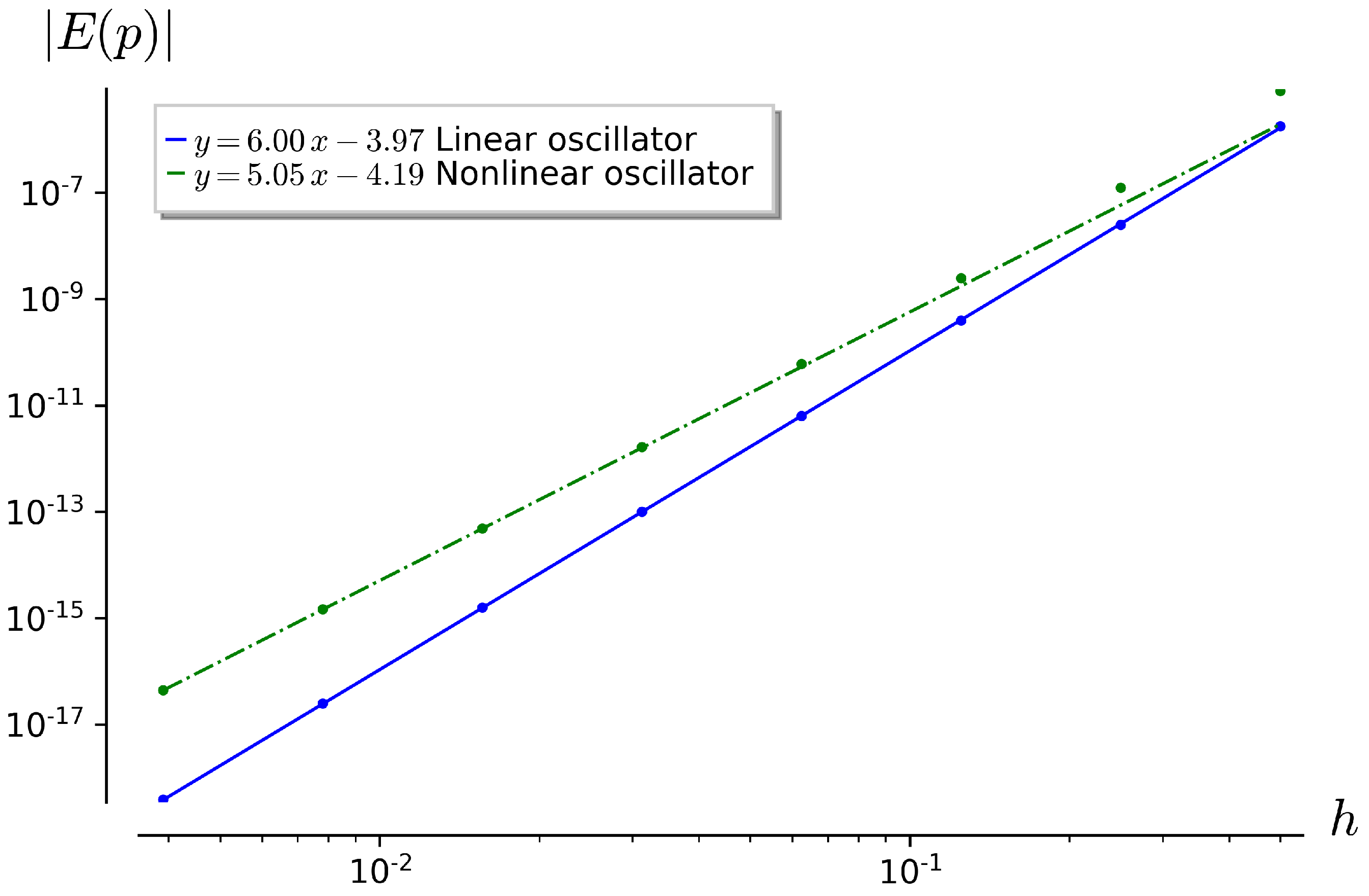
In calculations for a system describing a linear oscillator, we obtain a slope of the line in the linear part of the diagram that is approximately equal to six. However, for a nonlinear oscillator, for example, the Jacobi oscillator, the Shanks scheme will provide only the fifth order of approximation, which is shown in Figure 1.

Generally speaking, these figures indicate that the Shanks scheme can be recommended for application to linear systems of differential equations, checking the order using the Richardson method, and it cannot be recommended for nonlinear systems of differential equations.

Thus, the “scalarization” of the problem of finding the weights of the Runge–Kutta scheme can give us false values for the weights, which will be detected at the stage of application, when we will estimate the actual order of approximation. Moreover, such problems will be encountered for the first time in sixth-order schemes.

4. Simplifying the Problem of Determining the Weights of Difference Schemes

To simplify the problem, we need to give up something. We will give up the guarantee that all the found options for the values of the weights correspond to the assumed maximum of the order of approximation and will find weights only for the scalar equation:

$${\displaystyle \frac{dx}{dt}}=f\left(x\right),$$

(6)

with a polynomial right-hand side. In general, the polynomial can be of any degree; however, if we follow our concept of simplifying calculations, it makes sense to use polynomials of a low degree (not higher than three). We will find all variants of weight values that ensure the highest order of approximation for this class of differential equations and then apply the results found to vector and nonlinear systems of the form (1).

We propose the following algorithm for solving the problem of determining the weights of an explicit scheme. We are given the assumed order of approximation r, the field K, the polynomial f, and the following family of schemes:

$$\widehat{x}=x+g(x,\Delta t,a_0,\dots ),$$

(7)

where $a_0,\dots$ are symbolic variables, and g is a symbolic expression containing f. The algorithm for finding coefficients is as follows:

• The exact solution to the Cauchy problem is expanded in powers of $\Delta t$ up to $\Delta t^{r+1}$.
• The solution to Equation (7) with respect to $\widehat{x}$ is expanded in a Taylor series up to $\Delta t^{r+1}$.
• The coefficients of these two expansions are compared at the corresponding powers of $\Delta t$. The result is a system of equations with respect to $(a_0,\dots )$.
• If the system is compatible, then it is solved by finding the Gröbner basis. At the output, we obtain a set of coefficients from the field K.

5. Examples of the Algorithm Application

The algorithm described in the previous Section was implemented in the Sage system (https://github.com/vmkadrov/dps, accessed on 20 July 2024).

Let us start with the simplest example. We define the coefficients of the difference scheme as follows:

$$\widehat{x}=x+(af\left(x\right)+bf\left(\widehat{x}\right))\Delta t.$$

The conditions for this scheme to be a second-order scheme for the scalar Riccati equation are as follows:

$${\displaystyle \frac{dx}{dt}}=1+x^2$$

These are reduced to two algebraic equations:

$$a=b={\displaystyle \frac{1}{2}}.$$

This gives a trapezoid scheme, which, as is known, is indeed of the second order in all cases, including the vector one. The situation turns out to be paradoxical. In classical studies, the weights for difference schemes for systems of differential equations of a general type were sought, and a result was obtained that could be arrived at by considering one specific equation of the first order. It seems that by analogy with the concept of a point of general position, one can introduce the concept of a differential equation of a general position. The Shanks example, however, requires caution here.

As a second example, we will try to use the algorithm to create an explicit Runge–Kutta scheme of the fourth order with rational coefficients. To do this, we extend the (4) scheme to 4 stages:

$$\widehat{\mathbf{x}}=\mathbf{x}+b_1{\mathbf{f}}_1\Delta t+b_2{\mathbf{f}}_2\Delta t+b_3{\mathbf{f}}_3+b_4{\mathbf{f}}_4\Delta t,$$

(8)

where

$$\left\{\begin{array}{c}{\mathbf{f}}_1=\mathbf{f}\left(\mathbf{x}\right),\hfill \\ {\mathbf{f}}_2=\mathbf{f}(\mathbf{x}+a_{21}{\mathbf{f}}_1\Delta t),\hfill \\ {\mathbf{f}}_3=\mathbf{f}(\mathbf{x}+a_{31}{\mathbf{f}}_1\Delta t+a_{32}{\mathbf{f}}_2\Delta t),\hfill \\ {\mathbf{f}}_4=\mathbf{f}(\mathbf{x}+a_{41}{\mathbf{f}}_1\Delta t+a_{42}{\mathbf{f}}_2\Delta t+a_{43}{\mathbf{f}}_2\Delta t),\hfill \end{array}\right.$$

(9)

and $a_{21}\dots a_{43}$ and $b_1\dots b_4$ are symbolic variables. The conditions for this scheme to be of the fourth order are reduced to a system of algebraic equations, which we will not present here due to their complexity.

Among the equations obtained in this way, only a few coincide with the equations given in [2] (p. II.1.11). In order to compare both systems, it is necessary to calculate the Gröbner bases for both, which, as is well known, is a rather laborious task. We will limit ourselves here to the fact that the known set of coefficients for the Runge–Kutta scheme is its solution.

Table 2. Butcher’s table for the standard rk4 scheme.

$\frac{1}{2}$	$\frac{1}{2}$
${\displaystyle \frac{1}{2}}$	0	${\displaystyle \frac{1}{2}}$
1	0	0	1
	${\displaystyle \frac{1}{6}}$	${\displaystyle \frac{1}{3}}$	${\displaystyle \frac{1}{3}}$	${\displaystyle \frac{1}{6}}$

presents the solution of this system in the form of a Butcher table. Substituting these coefficients into the original rule, we obtain an explicit Runge–Kutta scheme of the fourth order. Thus, our system, in any case, is not overdetermined, and some of its roots coincide with the known roots of the second system.

It is clearly seen that the essence of the Runge–Kutta method is that only linear combinations and the $\mathbf{f}$ operation are calculated. It seems quite obvious that in the general case, this is very convenient and economical in comparison with the Adams method [6,7], which requires the calculation of derivatives. However, the differentiation operation in symbolic form is not always expensive, especially if ODEs with a polynomial right-hand side are considered.

From this point of view, it seems promising to develop methods that combine the ideas of the Runge–Kutta and Adams methods. It is worth saying that the convergence of the Runge–Kutta and Adams methods has been well studied [2]. In this paper, we will not provide rigorous proofs of the convergence of the proposed techniques, as this is inconsistent with the goal of quickly determining coefficients. Instead, we will focus on numerical experiments and evaluate the error order using the Richardson method.

For example, one can try to design a difference scheme of the following form:

$$\left\{\begin{array}{cc}\hfill \widehat{\mathbf{x}}=\mathbf{x}& +a_0\mathbf{f}\left(\mathbf{x}\right)\Delta t+a_{1}D\mathbf{f}\left(\mathbf{x}\right)\Delta t^2\hfill \\ \hfill & +a_2\mathbf{f}(\mathbf{x}+a_3\mathbf{f}\left(\mathbf{x}\right)\Delta t+a_{4}D\mathbf{f}\left(\mathbf{x}\right)\Delta t^2)\Delta t,\hfill \end{array}\right.$$

(10)

For $a_2=0$, we easily reach the second order. Considering the structure of the expression for this coefficient, we assume that by selecting $a_2\dots a_4$, we can reach the third order. Let $a_2\ne 0$. Then, to obtain the third order of approximation, it is necessary to solve the following system:

$$\left\{\begin{array}{c}{a}_2{a}_3+a_1-{\displaystyle \frac{1}{2}}=0,\hfill \\ a_1{a}_4+{\displaystyle \frac{1}{6}}{a}_3-{\displaystyle \frac{1}{2}}{a}_4=0,\hfill \\ a_2{a}_4-{\displaystyle \frac{1}{6}}=0,\hfill \\ a_0+a_2-1=0.\hfill \end{array}\right.$$

(11)

The Gröbner basis of this system in lex-order gives an equivalent system with three equations:

$$\left\{\begin{array}{c}{a}_0+a_2-1=0,\hfill \\ a_1+a_2{a}_3-{\displaystyle \frac{1}{2}}=0,\hfill \\ a_2{a}_4-{\displaystyle \frac{1}{6}}=0.\hfill \end{array}\right.$$

(12)

The last two equations show that the system has an infinite number of solutions, since all 5 coefficients are uniquely determined by selecting two of them. Thus, we are dealing with a certain surface in the space of coefficients. Let us select several solutions of this system (

Table 3. Solution to system (12).

${\mathit{a}}_0$	${\mathit{a}}_1$	${\mathit{a}}_2$	${\mathit{a}}_3$	${\mathit{a}}_4$
${\displaystyle \frac{6}{9}}$	${\displaystyle \frac{1}{6}}$	${\displaystyle \frac{3}{9}}$	1	${\displaystyle \frac{1}{2}}$
${\displaystyle \frac{1}{4}}$	0	${\displaystyle \frac{3}{4}}$	${\displaystyle \frac{2}{3}}$	${\displaystyle \frac{2}{9}}$

). Verification using our algorithm showed that all sets, when substituted, yielded a third-order scheme.

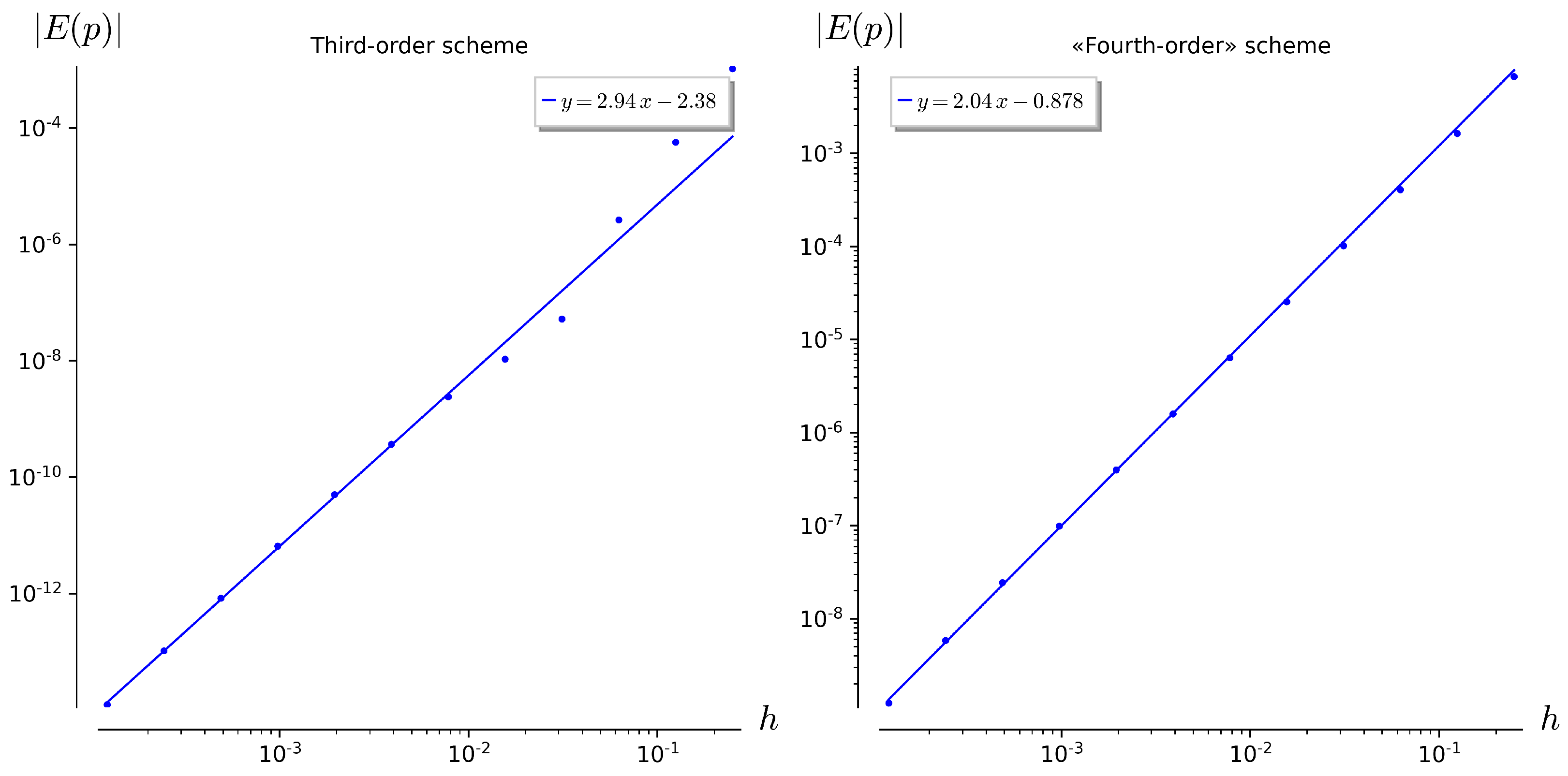
Applying Scheme (10) using the weights from Table 3 to systems of differential equations describing linear and nonlinear oscillators, we found that the slopes of the Richardson diagram in both cases were equal to 3 (see Figure 2), i.e., our strategy, when applied to schemes containing the differentiation operator, made it possible to easily find third-order schemes.

Let us construct a fourth-order scheme in a similar manner:

$$\left\{\begin{array}{cc}\hfill \widehat{\mathbf{x}}=\mathbf{x}& +a_0\mathbf{f}\left(\mathbf{x}\right)\Delta t+a_{1}D\mathbf{f}\left(\mathbf{x}\right)\Delta t^2\hfill \\ \hfill & +a_2\mathbf{f}(\mathbf{x}+a_3\mathbf{f}\left(\mathbf{x}\right)\Delta t+a_{4}D\mathbf{f}\left(\mathbf{x}\right)\Delta t^2)\Delta t\hfill \\ \hfill & +a_5\mathbf{f}(\mathbf{x}+a_6\mathbf{f}\left(\mathbf{x}\right)\Delta t+a_{7}D\mathbf{f}\left(\mathbf{x}\right)\Delta t^2+a_{8}D\left(D\mathbf{f}\left(\mathbf{x}\right)\right)\Delta t^3)\Delta t,\hfill \end{array}\right.$$

(13)

Here, as in the case of the third-order scheme, the solution of the system is not a finite set of points; it is a manifold of dimension 4. Let us select one set of coefficients and test it using various examples.

For systems of linear differential equations, it showed the fourth order of approximation, but in the nonlinear case, the order turned out to be smaller. Figure 2 shows the Richardson diagrams for the third- and fourth-order schemes in calculations for the Jacobi oscillator system. The scheme that gave the fourth order for scalar problems turns out to be worse than the third-order scheme. We will discuss this particular scheme in detail and explore its notable aspects.

Now, we consider another example of a nonlinear dynamical system, the Rössler system [14].

$$\left\{\begin{array}{cc}\hfill \dot{x}& =-(y+z)\hfill \\ \hfill \dot{y}& =x+ay\hfill \\ \hfill \dot{z}& =b+z(x-c),\hfill \end{array}\right.$$

(14)

This system can be a model for describing an abstract chemical reaction [15]. We aim to test our hypothesis using this model, which consists of two linear equations and only one nonlinear equation. It is convenient for us because we can easily linearize the system by assuming that $z=0$

$$\left\{\begin{array}{cc}\hfill \dot{x}& =-y\hfill \\ \hfill \dot{y}& =x+ay,\hfill \end{array}\right.$$

(15)

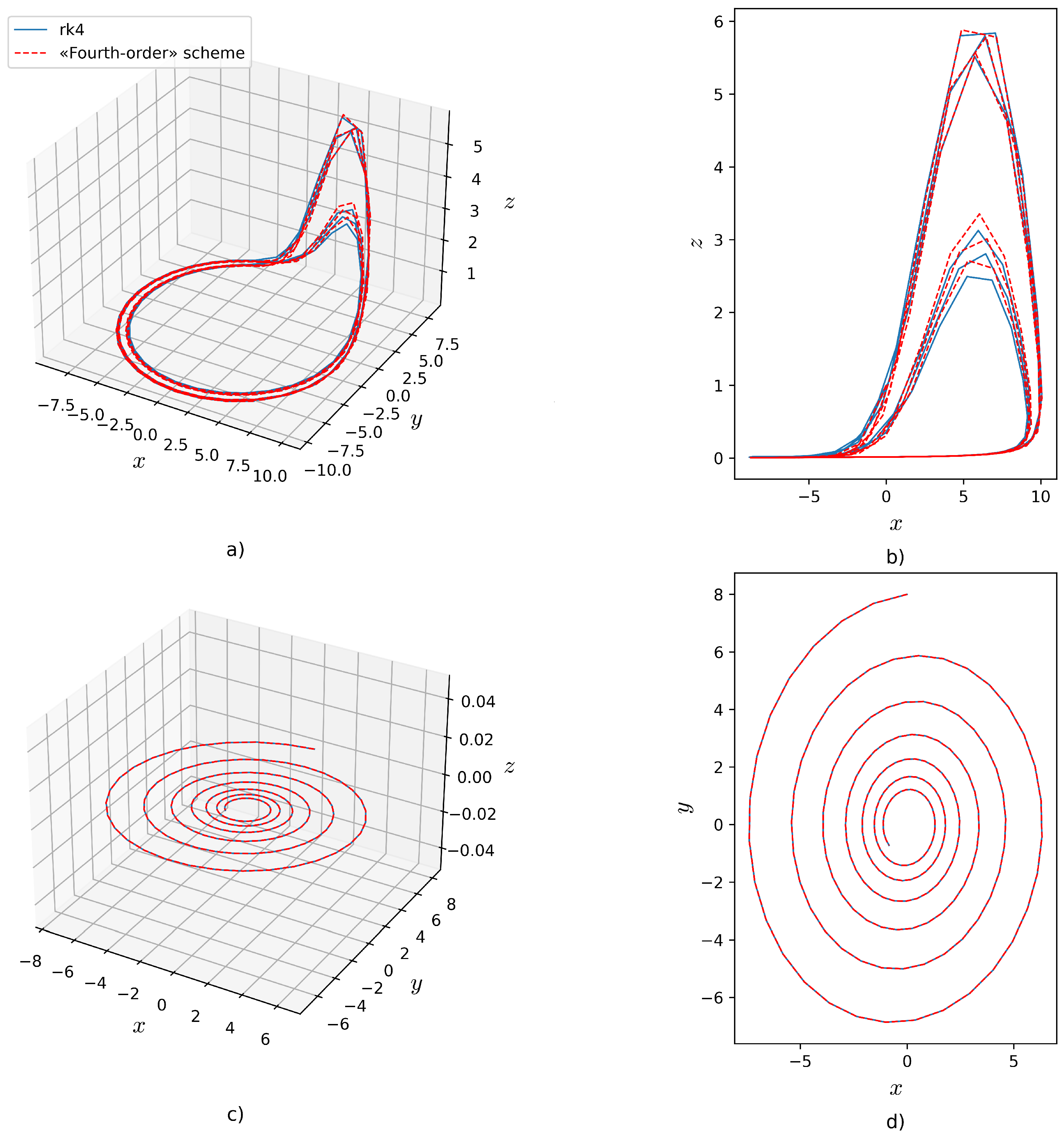
Thus, we check whether our scheme (13) gives a worse result for nonlinear examples than it should. In Figure 3, the solutions of the system are presented using the standard RK4 method and the proposed approach. It should be noted that, with the standard parameters (Figure 3a,b) and, consequently, the presence of a nonlinear component, there is a difference between the standard and new techniques. 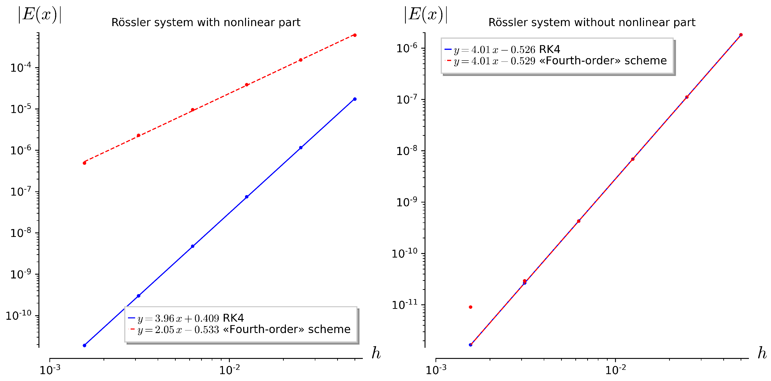However, in the linearized system (Figure 3c,d), this difference is less noticeable. As in the previous examples, Richardson’s method will be used to estimate the order of approximation (Figure 4). Here, we can make sure that, in the nonlinear case, the slope of the line in the diagram for our scheme is less than expected. Nevertheless, this scheme provides an assumed order of approximation when solving linear systems.

Thus, the phenomenon that was first discovered in the study of the Shanks scheme (see Section 3) is repeated for schemes of the form given in Equation (13), which contains differentiation.

6. Conclusions

In this paper, we considered the problem of determining the weights of difference schemes whose type is specified by a particular symbolic expression, and the order of approximation is equal to a given number. To solve the problem, it was proposed to proceed from considering systems of differential equations of a general type to a single scalar equation. This technique works well for low-order schemes. Reducing the order of a scheme whose weights are selected for a scalar problem when moving to a vector and nonlinear problem was first proposed in a study of the Shanks scheme, and it is reproduced with enviable regularity in other cases. This does not deteriorate our strategy for simplifying the problem of determining weights, which should include a clause on mandatory testing of the order using the Richardson method.

If the user of our FDM for the Sage system specifies the desired type of difference scheme and the number of weights is not very large (up to ten), then we already have software that automatically creates a system of algebraic equations for the weights, and the Sage built-in tools offer the user several options for the values of the weights to choose from. The user is left to choose one of the options at random and solve the differential equation of interest numerically. The slope of the Richardson diagram will tell him whether the option was chosen successfully or whether it is better to try the next one.

Generalization of this technique to the case of a large number of weights and, consequently, high-order schemes runs into purely algebraic difficulties in solving systems of nonlinear equations with dozens of unknowns. The Buchberger algorithm [16] used to solve them yields a solution in a finite number of steps, but this can take many hours or even days [17]. We see prospects for developing this approach in a different direction. Instead of defining all the weights to maximize the order of approximation, we can leave some of them undefined at the first stage. Then, we use this uncertainty to construct a difference scheme that not only approximates a given differential equation but also inherits its algebraic properties; for example, certain algebraic integrals of motion. This can be viewed as a generalization of the concept of the so-called explicit conservative Runge–Kutta schemes [18,19,20].