Optimization of Sensor Placement for a Measurement System for the Determination of Local Magnetic Material Properties

Abstract

The aim of this work is to optimize the sensor positions of a sensor–actuator measurement system for identifying local variations in the magnetic permeability of cut steel sheets. Before solving the actual identification problem, i.e., finding the material distribution, the sensor placement of the measurement setup should be improved in order to reduce the uncertainty of the identification of the material distribution. The Fisher information matrix (FIM), which allows one to quantify the amount of information that the measurements carry about the unknown parameters, is used as the main metric for the objective function of this design optimization. The forward problem is solved by the finite element method. The results show that the proposed method is able to find optimal sensor positions as well as the minimum number of sensors to achieve a desired maximum parameter uncertainty.

1. Introduction

The magnetic properties of electrical steel sheets play a crucial role in determining their performance in applications such as transformers, motors, and generators [1]. These properties, including magnetic permeability, saturation magnetization, and hysteresis characteristics, can vary locally across the material due to the influence of different manufacturing processes. Cutting techniques are particularly important in shaping and creating the desired geometry of electrical steel sheets for various applications. However, these cutting processes can cause changes in the microstructure and residual stresses at the cut edges, leading to a deterioration in the magnetic material properties.

The extent of this deterioration depends on the specific cutting process, e.g., punching, laser cutting, or water-jet cutting and the cutting parameters that can be the laser intensity, blade sharpness, or cutting speed [2,3,4]. Also, electrical discharge machining is also a well-known cutting process and probably has the least effect on material properties, but it is rarely used in industry as it is slow and expensive. Accurately and efficiently determining the local properties affected by the cut edges is a challenging task that continues to be actively explored by the scientific community.

One commonly used approach involves dividing the electrical steel sheet into multiple narrower strips, where the combined width of these strips reflects the dimensions of the original sheet. By modifying the strip width, different combinations of the cutting length to bulk material ratio can be evaluated using a single sheet tester or an Epstein frame [5,6].

There are both destructive and nondestructive methods for measuring the influence of cut edges, as presented by [7,8,9,10]. The destructive method involves drilling holes in the sheets and placing search coils near the cut edges to measure the magnetic flux. The nondestructive method utilizes the needle probe method. But in all cases, either the sheet is destroyed or a homogenization method is used.

Since there is no noninvasive method available that can accurately determine the local degradation of cut steel sheets, we aim to comprehensively investigate the impact of cut edges on the magnetic material properties by integrating various scientific methodologies. This involves the combination of measurement, numerical simulation, and inverse modeling techniques. This work is about an optimization of the setup before it is actually built; therefore, the entire measurement process is described in the following, but the investigations in this work are limited to the use of synthetic data based on numerical simulations. To gather measurement data, we use a sensor–actuator (SA) system to locally magnetize electrical steel sheets and measure the magnetic field above the sample. To solve the inverse problem, an appropriate model of the SA system and electrical steel sheets is set up, and the magnetostatic problem is solved by the finite element (FE) method. The parameters of the material model reflecting the degradation caused by cutting are then identified by minimizing the mismatch between the measured data and the simulated data. The first investigations on solving the inverse problem using the described method and synthetic measurement data are presented in [11].

However, solving an ill-posed inverse problem is generally a challenging task, and obtaining the right data is crucial. Before the measurement system is actually built, studies should be carried out on the reliability and accuracy of the identification method. In fact, the number of sensors is limited and the spatial resolution is determined by their size. Thus, the aim of this study is to optimize the sensor positions in order to solve the inverse problem as accurately as possible, thereby minimizing the uncertainty of the solution (i.e., the identifiable parameters). Determining the uncertainties of an inverse problem involves, in general, calculating how measurement noise affects the parameter space.

In this study, only random, normally distributed measurement noise is considered, while the uncertainty of the model (i.e., comparing actual measurement data with simulation data to solve the inverse problem) is disregarded as only simulation data are available and biases and systematic effects are also neglected. The uncertainties can be calculated using the covariance matrix, which represents the dispersion of the identified parameters obtained from multiple independent samples of noisy measurement data and an inverse scheme.

Since the parameter identification includes solving the FE problem several times, the covariance determination for a significant number of samples is computationally highly intensive. Therefore, the Fisher information matrix (FIM) is used, which is an estimate of the inverse covariance matrix and is determined with only a few model evaluations. By definition, the FIM is the Hessian matrix of the negative log-likelihood function given some measurement data and therefore describes the curvature of the probability density of observed data as a function of the model parameters [12]. The higher the curvature around the maximum is, the lower the variance of the parameters to be identified. Thus, the Hessian is computed using the Jacobian of the model output with respect to the identification parameters and is used to assess the parameter uncertainty. An extensive description of the relation between response surfaces and parameter uncertainties is presented in [13]. It is worth mentioning that an identifiability analysis, which answers the question if the solution is unique, is not within the scope of this work. In our methods, the parameter uncertainty is evaluated assuming that the estimate is in the proximity of the true solution.

The Fisher information matrix (FIM) is used to calculate the parameter uncertainty for the model with the corresponding model parameters defining the sensor configuration. To minimize the resulting uncertainty, a design of experiment optimization is applied. This means that the parameter variances of the FIM form the single objective function of the model optimization with different approaches to describing optimality. D-, A-, and E-optimality are distinguished, evaluating either the determinant, trace, or eigenvalues of the FIM, thus defining different objectives for the underlying problem. In this work, different objectives are tested and compared to find an optimal sensor placement.

In the literature, similar methods for finding an optimal design of experiment for the purpose of accurately identifying model parameters and by using the information provided by the FIM are used for different fields of applications. For instance, in [14], an optimal design for the estimation of the parameters of an electronic chip cooling system is found. In the field of structural health monitoring, where changes to the material and geometric properties of engineering structures such as bridges and buildings are monitored, an optimal sensor placement is crucial, and therefore, corresponding works can be found in [15,16].

This paper is structured as follows. Section 2 describes the concept of the measurement setup and the computational model of the sensor–actuator system. In Section 3, the parameter identification problem is introduced and the Fisher information matrix and its relation to the parameter uncertainty is shown. Also, the concept of the Cramér–Rao Bound describing the lower bound of the variance of a parameter estimator is explained in this section. The setup for optimizing the sensor placement is described in Section 4, which incorporates also the formulation of different objective functions. Lastly, Section 5 presents the results containing a sensitivity analysis and optimized sensor positions using different objective functions.

2. Sensor–Actuator System

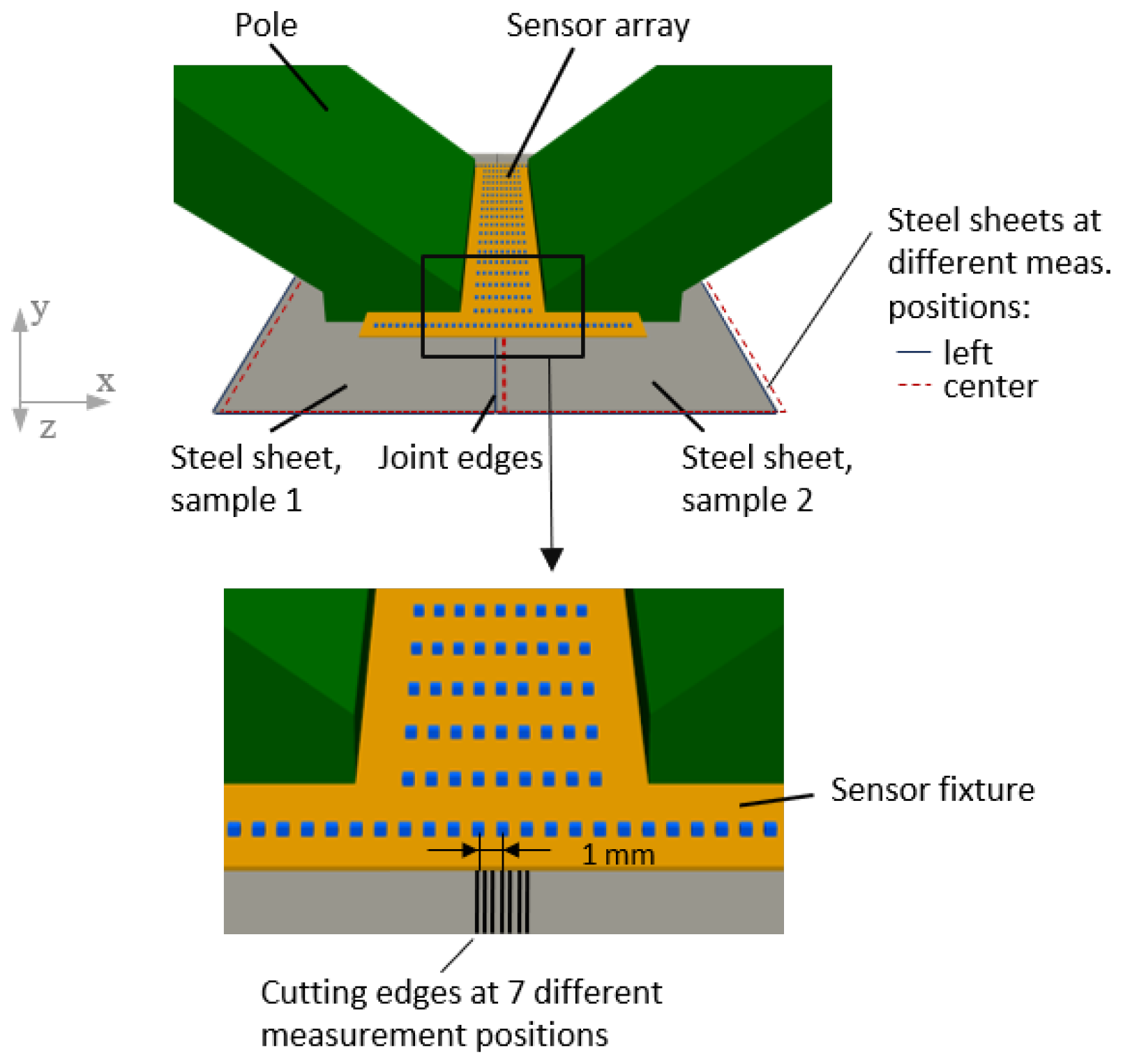
The model of the sensor–actuator system is shown in Figure 1 and consists of an iron core, excitation coils which generate a magnetic field, two steel sheet samples, and a sensor array.

Figure 1. Front view of the 3D model of the sensor–actuator system.

The x-, y-, and z-components of the magnetic field are measured above the steel sheet samples and depend on the distribution of the magnetic permeability of the material. To ensure a sufficient sensitivity of the magnetic field changes due to material inhomogeneity, two samples are placed close to each other along the cut edge [11]. Assuming that both samples come from the same batch and adhere to identical cutting process parameters, it is reasonable to consider their material behavior as identical.

The magnetic field is captured by $n_{\mathrm{s}}$ sensors, which are fixed to the sensor–actuator system. In order to increase the amount of data and thus improve the information gain and accuracy, the sensor–actuator system is positioned at $n_{\mathrm{p}}$ different locations along the x direction, which means orthogonal to the cutting edge or the interface of sample 1 and 2, see Figure 2. This enables a higher resolution in the area of the cut edge, which cannot be achieved with the use of additional sensors due to their minimal size. Thus, $n_{\mathrm{p}}·n_{\mathrm{s}}$ data points are collected in a measurement series. To ensure consistency, the sheets will be demagnetized between each measurement position to eliminate any residual magnetism. This assumption is crucial for subsequent numerical simulations.

Figure 2. Detailed view of the measurement setup showing the sensor array and different measurement positions realized by moving the sensor–actuator system relative to the steel sheets. The distance between two sensors is 1 mm in the x direction and the measuring positions are chosen equidistantly ±1 mm around the middle sensor. For better illustration, only two measuring positions are shown in the upper figure, and the steel sheets are moved instead of the sensor–actuator system.

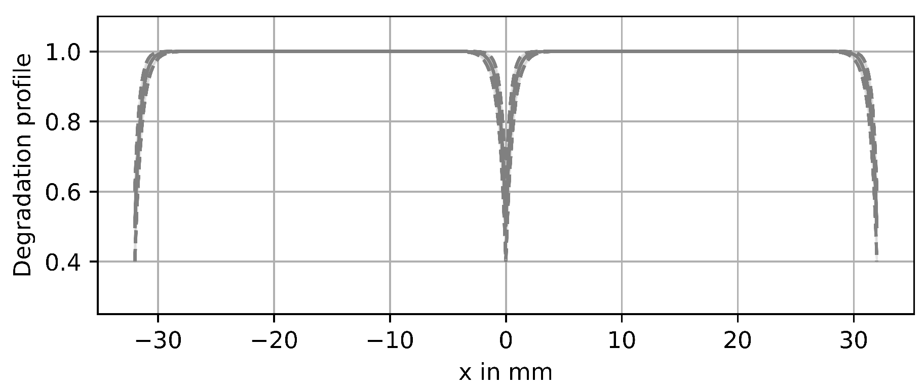
The degradation profile of steel due to punching is taken from the literature [17]. It follows an exponential function, where the unknowns are the initial value $\widehat{\gamma }$ at the cut edge and the degradation skin depth $\delta$,

$$\begin{array}{c}\hfill \gamma \left(x\right)=1-(1-\widehat{\gamma }){\mathrm{e}}^{-x/\delta }.\end{array}$$

(1)

Figure 3 shows the degradation profiles of two cut and juxtaposed samples produced from two different steel sheets with a width of $36\mathrm{mm}$.

Figure 3. Permeability distribution along two juxtaposed samples for two different materials.

Thus, the permeability distribution starts at the cut edge at $x=0$ and saturates to a constant permeability ${\mu }_{\mathrm{ref}}$,

$$\begin{array}{c}\hfill \mu \left(x\right)={\mu }_{\mathrm{ref}}\gamma \left(x\right).\end{array}$$

(2)

In the FE model, the two samples are modeled as a single sheet with the material model, as shown in Figure 3.

The magnetostatic field is computed by the finite element method (FEM) solving the following partial differential equation (PDE):

$$\begin{array}{c}\hfill \nabla \times {\displaystyle \frac{1}{\mu }}\nabla \times \mathbf{A}-\mathbf{J}=\mathbf{0},\end{array}$$

(3)

for the magnetic vector potential $\mathbf{A}$ with a given electric current density $\mathbf{J}$. Having solved the PDE, the magnetic field $\mathbf{B}$ at all sensor positions can be computed by

$$\begin{array}{c}\hfill \mathbf{B}=\nabla \times \mathbf{A}.\end{array}$$

(4)

The computational domain is discretized by 40,084 tetrahedral elements, and the FEM solution is obtained by the open-source software openCFS, version 24.03 [18]. For the excitation, a current density of $J=2\mathrm{kA}/{\mathrm{m}}^2$ is assigned. The magnetic material model is assumed to be linear in this work.

3. Parameter Identification and Uncertainty

Parameter identification is the process of adjusting model parameters until the model output matches the observed or measured data. This process typically includes conducting numerical optimization techniques, such as least squares fitting or maximum likelihood estimation, while using real measured data. Since, in this work, the sensitivity of the measurement system should be improved and it is not the aim to actually identify the parameters, simulated data are used for the measurements instead of real data.

The likelihood for an identification parameter state $\mathbf{\theta }$ given n measurements taken in a single experiment is

$$\begin{array}{c}\hfill L\left(\mathbf{\theta }\right|\mathbf{d})={\left(2\pi {\sigma }_{\mathrm{d}}^2\right)}^{-n/2}exp\left(-{\displaystyle \frac{1}{2{\sigma }_{\mathrm{d}}^2}}\sum _{i=1}^n\left(f_i\left(\mathbf{\theta }\right)-d_i{)}^2\right)\right),\end{array}$$

(5)

where $f\left(\mathbf{\theta }\right)$ is the model and $\mathbf{d}$ is the vector of the measured data. It is assumed that all sensors have the same Gaussian noise level ${\sigma }_{\mathrm{d}}$. In practice, the log-likelihood function is used for the sake of computational ease.

Basically, there are two concepts to optimize the sensor positions. The first one is to predefine a number of sensors and change their continuous position. Due to the fact that the sensors are considered as volumes in the FE model, a position change requires remeshing and the computation of the FEM solution. Instead, a 2D sensor array can be defined in advance, where the values of all sensors are evaluated with only one FEM computation, and the optimization procedure takes the active or inactive status of each sensor as a parameter. Thus, we introduce binary weights $\mathbf{w}\in {\{0,1\}}^{n_{\mathrm{s}}}$ such that $w_k=1$ if and only if sensor k is used. As described in Section 2, the sensor–actuator system is positioned at different locations along the x direction, which means that the cut edge is shifted relative to the sensors. For all measurement positions, the same sensor configuration, i.e., the same set of weights $\mathbf{w}$, is used. Thus, with $n_{\mathrm{p}}$ being the number of measurement positions, the log-likelihood function is written as

$$\begin{array}{c}\hfill l\left(\mathbf{\theta }\right|\mathbf{d})=-{\displaystyle \frac{n}{2}}ln\left(2\pi {\sigma }_{\mathrm{d}}^2\right)-\sum _{k=1}^{n_{\mathrm{s}}}\sum _{j=1}^{n_{\mathrm{p}}}\left({\displaystyle \frac{w_k}{2{\sigma }_{\mathrm{d}}^2}}{\left(f_{jk}\left(\mathbf{\theta }\right)-d_{jk}\right)}^2\right),\end{array}$$

(6)

with $n=n_{\mathrm{p}}\sum w_k$.

The maximizer of the log-likelihood function is the estimated parameter vector ${\mathbf{\theta }}^{*}$, fitting the model to the observed noisy data:

$$\begin{array}{c}\hfill {\mathbf{\theta }}^{*}=arg\underset{\mathbf{\theta }}{max}l\left(\mathbf{\theta }\right|\mathbf{d}).\end{array}$$

(7)

The maximum likelihood estimate can be found by applying a suitable optimization method. However, the optimization of the problem formulated in (7) leads to different estimated parameters for different independent measurements due to the data noise. Thus, the data noise leads to uncertainties in the parameter space. These uncertainties can be evaluated by taking a significant amount of noisy data sets and calculating the covariance matrix of the estimated parameters. However, this process is computationally very expensive since the inverse problem must be solved for each set. Therefore, another method is used, which estimates the covariance matrix by evaluating the Hessian of the log-likelihood function.

3.1. Fisher Information Matrix

The Fisher information matrix, denoted as $\mathrm{I}\left(\mathbf{\theta }\right)$, is a mathematical quantity commonly used in maximum likelihood estimation (MLE). In the context of MLE, it represents the amount of information that the observed data contain about the parameter vector $\mathbf{\theta }$. It is defined as the negative expectation of the second derivative of the log-likelihood function with respect to $\mathbf{\theta }$ [12],

$$\begin{array}{c}\hfill \mathrm{I}\left(\mathbf{\theta }\right)=-\mathrm{E}\left[{\displaystyle \frac{{\partial }^{2}l\left(\mathbf{\theta }\right|\mathbf{d})}{\partial {\mathbf{\theta }}^2}}\right],\end{array}$$

(8)

and quantifies the curvature or shape of the log-likelihood function near the true value of the parameter vector.

The FIM for two parameters a and b and the residuals $r_i=f_i\left(\mathbf{\theta }\right)-d_i$ can be written as

$$\begin{array}{c}\hfill \mathrm{I}\left(\mathbf{\theta }\right)=-\mathrm{E}\left[-{\displaystyle \frac{1}{{\sigma }_{\mathrm{d}}^2}}\sum _{i=1}^n{\displaystyle \frac{\partial r_i\left(\mathbf{\theta }\right)}{\partial {\mathbf{\theta }}_{\mathrm{a}}}}{\displaystyle \frac{\partial r_i\left(\mathbf{\theta }\right)}{\partial {\mathbf{\theta }}_{\mathrm{b}}}}+\sum _{i=1}^n{r}_i\left(\mathbf{\theta }\right){\displaystyle \frac{{\partial }^2{r}_i\left(\mathbf{\theta }\right)}{\partial {\mathbf{\theta }}_{\mathrm{a}}\partial {\mathbf{\theta }}_{\mathrm{b}}}}\right].\end{array}$$

(9)

At the best-fit ${\mathbf{\theta }}^{*}$, the residuals are very small, and therefore, the second term of (9) can be neglected. Thus, the approximated observed FIM is calculated by

$$\begin{array}{c}\hfill \mathrm{I}\left({\mathbf{\theta }}^{*}\right)={\displaystyle \frac{1}{{\sigma }_{\mathrm{d}}^2}}\left(\mathrm{J}{\left({\mathbf{\theta }}^{*}\right)}^{\mathrm{T}}\mathrm{J}\left({\mathbf{\theta }}^{*}\right)\right)\end{array}$$

(10)

using the Jacobian $\mathrm{J}\left({\mathbf{\theta }}^{*}\right)$. The inverse of the Fisher information matrix is an estimator of the asymptotic covariance matrix,

$$\begin{array}{c}\hfill \mathrm{\Sigma }\left({\mathbf{\theta }}^{*}\right)\approx \mathrm{I}{\left({\mathbf{\theta }}^{*}\right)}^{-1},\end{array}$$

(11)

and the parameter variances are then the diagonal elements of $\mathrm{\Sigma }\left({\mathbf{\theta }}^{*}\right)$; thus,

$$\begin{array}{c}\hfill \mathrm{I}{\left({\mathbf{\theta }}^{*}\right)}^{-1}=\left[\begin{array}{ccc}{\sigma }_{{\theta }_1}^2& \cdots & {\sigma }_{{\theta }_1}{\sigma }_{{\theta }_{\mathrm{m}}}\\ ⋮& \ddots & ⋮\\ {\sigma }_{{\theta }_1}{\sigma }_{{\theta }_{\mathrm{m}}}& \cdots & {\sigma }_{{\theta }_{\mathrm{m}}}^2\end{array}\right].\end{array}$$

(12)

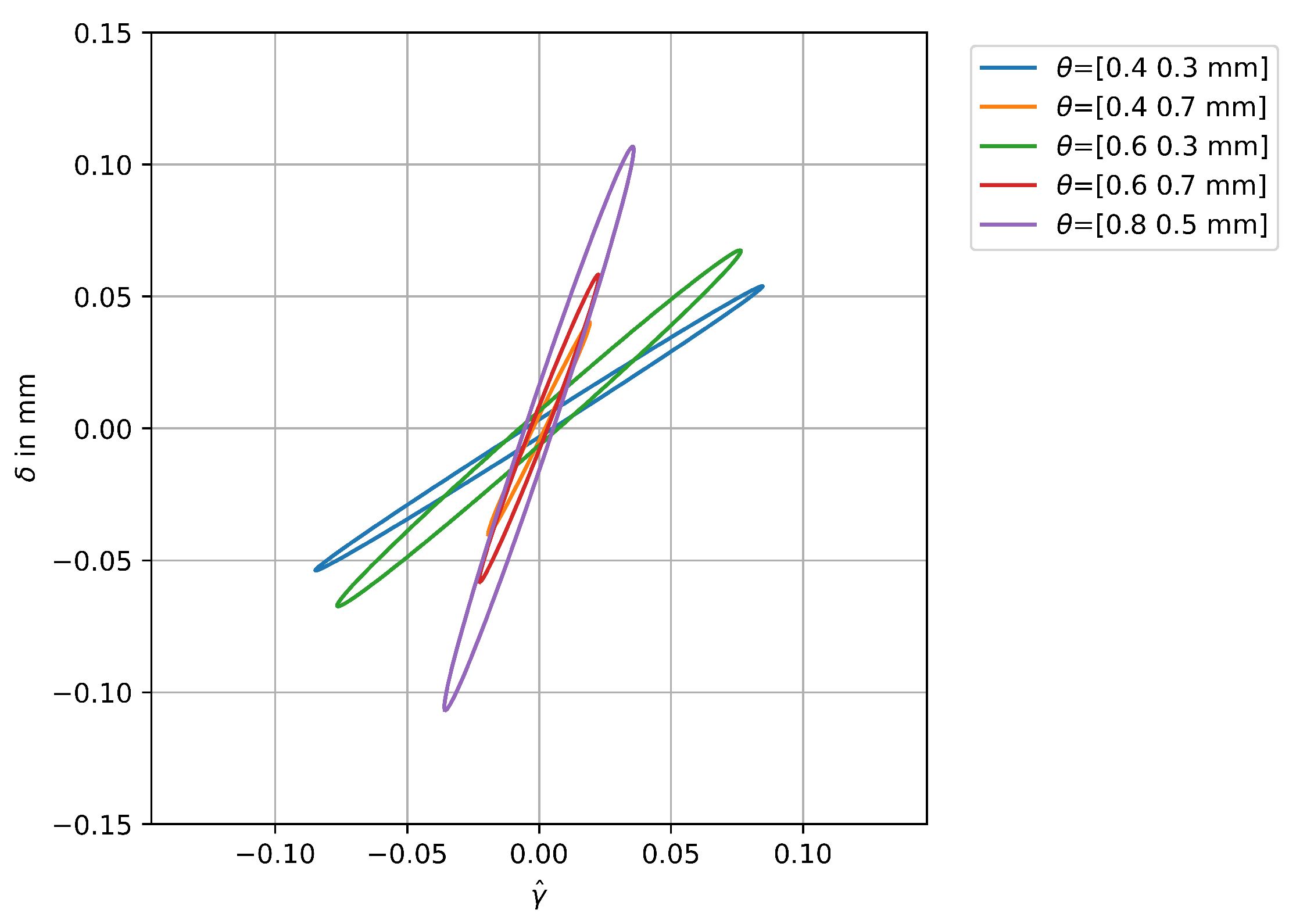
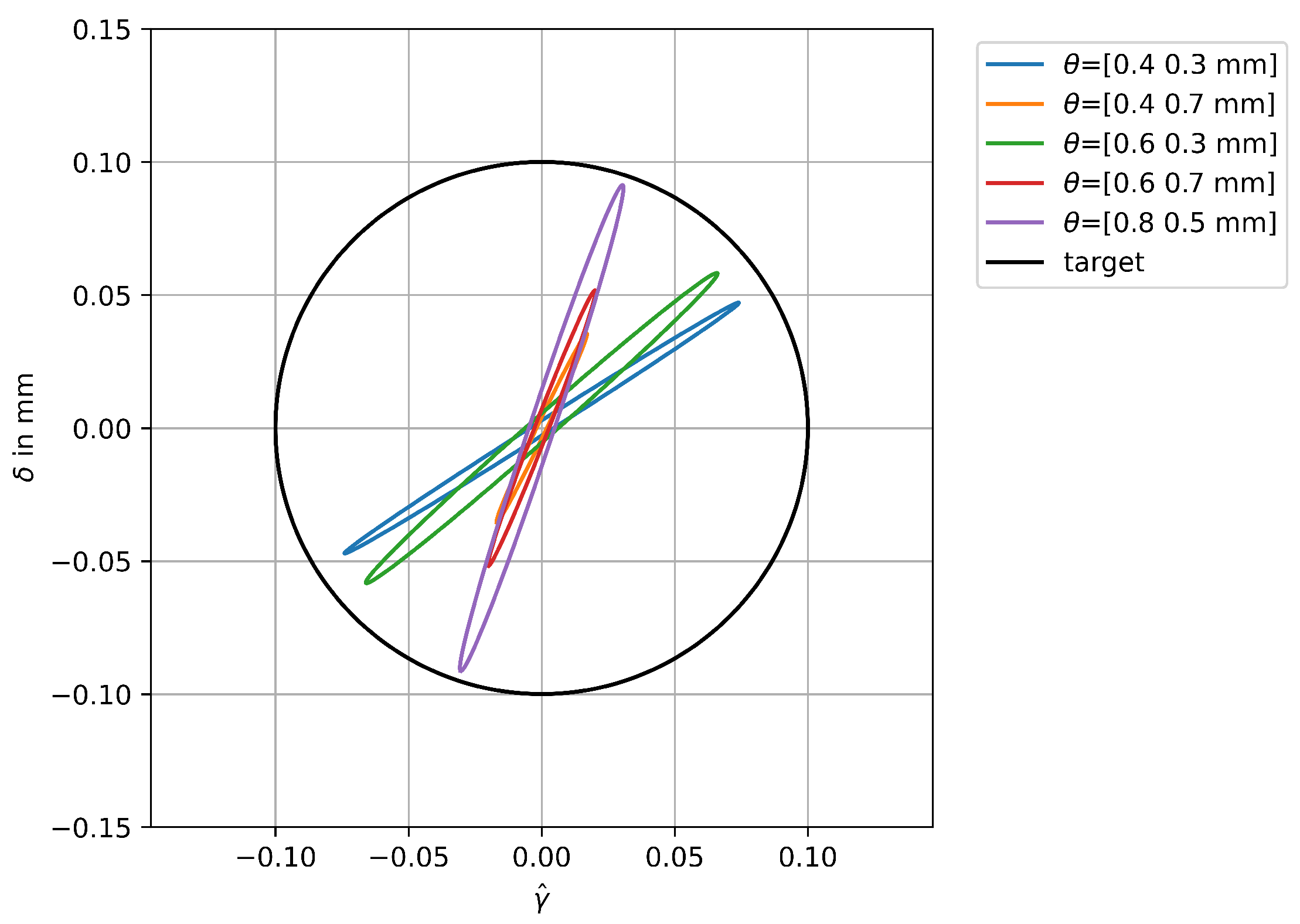
3.2. Cramér–Rao Bound and Target Variance of the MLE

The Cramér–Rao Bound (CRB) is a fundamental concept in statistical estimation theory [19]. It provides a lower bound for the variance of an estimator for a parameter in a statistical model and thus the best possible accuracy that can be achieved with the present model and the available measurements. The CRB is given by the inverse of the Fisher information matrix,

$${\sigma }_{{\widehat{\theta }}_i}^2\ge {\mathrm{I}}_{ii}{\left({\mathbf{\theta }}^{*}\right)}^{-1},$$

(13)

with $\widehat{{\theta }_i}$ being an estimate of the i-th parameter of the set $\mathbf{\theta }$. Therefore, the following condition must hold for a target variance ${\sigma }_{\mathrm{t},i}^2$:

$${\sigma }_{\mathrm{t},i}^2-{\mathrm{I}}_{ii}{\left({\mathbf{\theta }}^{*}\right)}^{-1}\ge 0.$$

(14)

For a confidence level $100(1-\alpha )\%$, with $\alpha$ being the significance level; the confidence interval can be written as

$$\begin{array}{c}\hfill \mathrm{CI}=\left({\theta }^{*}-z\sigma ,{\theta }^{*}+z\sigma \right),\end{array}$$

(15)

where the z-score is $1.96$ for a confidence level of $95\%$. Thus, the target variance for a maximum deviation $\mathrm{\Delta }{\theta }_{\mathrm{t}}$, which is defined by the designer, can be calculated by

$${\sigma }_t={\displaystyle \frac{\mathrm{\Delta }{\theta }_{\mathrm{t}}}{z}}$$

(16)

meaning that

$${\mathrm{I}}_{ii}{\left({\mathbf{\theta }}^{*}\right)}_{\mathrm{t},i}^{-1}<{\left({\displaystyle \frac{\mathrm{\Delta }{\theta }_{\mathrm{t}}}{z}}\right)}^2$$

(17)

must be fulfilled.

4. Sensor Position Optimization

The optimal design of experiments (DoE) approach deals with the task of finding an optimal experimental configuration such that the reliability of the estimated model parameters is maximized. In the case at hand, this task simplifies to determining optimal sensor positions. As described in Section 3, a 2D sensor array is provided and each sensor can be active or inactive. Therefore, the optimization parameters are the binary weights $\mathbf{w}\in {\{0,1\}}^{n_{\mathrm{s}}}$, where $n_{\mathrm{s}}$ is the number of sensors in the predefined sensor array. The number and the locations of the measurement positions are fixed and are not part of the parameter space.

4.1. Objective Function

It has been shown that the FIM can be used to assess the reliability of the parameter estimation. However, for the optimization procedure, a matrix can not be directly used, and a single-valued design function is needed instead. In general, there are different approaches to how to combine the information of the covariance matrix into a single-valued function. The most prominent ones according to [20] are

• A-criterion: the trace of the covariance matrix, $C_{\mathrm{A}}\left(\mathrm{\Sigma }\right)=\mathrm{trace}\left(\mathrm{\Sigma }\right)$;
• D-criterion: the determinant of the covariance matrix, $C_{\mathrm{D}}\left(\mathrm{\Sigma }\right)=\det \left(\mathrm{\Sigma }\right)$;
• E-criterion: the maximal eigenvalue of the covariance matrix, $C_{\mathrm{E}}\left(\mathrm{\Sigma }\right)={\lambda }_{\max }\left(\mathrm{\Sigma }\right)$.

The D-criterion is favored due to its connection to the volume of the confidence ellipsoid and its invariance with respect to transformations applied to the model parameters. However, it tends to emphasize the most sensitive parameter, which could be a drawback depending on the problem [21]. The A-criterion requires scaling of model parameters to achieve meaningful results. Its major drawback is its ignorance of the information gained from the off-diagonal elements of the covariance matrix, which becomes inefficient when there is a high correlation between parameters. While E-optimality might lead to a slight increase in the volume of the confidence ellipsoid, the E-criterion effectively reduces the largest semi-axis of the confidence ellipsoid. Since it is important to reduce the uncertainties of both material parameters to a tolerable value, the E-optimality is used for the underlying problem. The objective function is therefore formulated as

$$C_{\mathrm{E}}(\mathbf{w},\mathbf{\theta })={\lambda }_{\max }\left(\mathrm{I}{(\mathbf{w},\mathbf{\theta })}^{-1}\right).$$

(18)

In order to optimize the sensor positions not only for a particular sample but for the entire domain of possible material parameters to be estimated, various estimators, i.e., different combinations of $\widehat{\gamma }$ and $\delta$ and their corresponding FIM, must be computed. Thus, the objective function includes a set of $n_{\mathrm{m}}$ different material distributions ${\mathbf{\theta }}_{1\dots {\mathrm{n}}_{\mathrm{m}}}$ that are uniformly distributed within $\widehat{\gamma }=[0,1]$ and $\delta =[0\mathrm{mm},1\mathrm{mm}]$, respectively. Thus, the optimal experimental design problem is formulated as

$$\begin{array}{ccc}\hfill \underset{\mathbf{w}\in {\mathbb{B}}^{n_{\mathrm{s}}}}{min}& & \sum _i^{n_{\mathrm{m}}}{C}_{\mathrm{E}}(\mathbf{w},{\mathbf{\theta }}_i).\hfill \end{array}$$

(19)

The flowchart of the optimization procedure is shown in Figure 4.

Figure 4. Flowchart of the optimization procedure.

4.2. Optimization Strategy

To find the global optimum of the problem, a stochastic optimization strategy, namely the Genetic Algorithm (GA), is used for the single-objective problem at hand. Due to the fact that sensors can be active or inactive, a binary version of the GA with a random initial population, half-uniform binary crossover, and bitflip mutation is used [22].

So, the parameters are defined to be a set of $n_{\mathrm{s}}$ binary values, $\mathbf{w}\in {\mathbb{B}}^{n_{\mathrm{s}}}$, where $w_i=1$ means that the sensor i is active. For constraint handling, the method of constraint violation (CV) as an objective is used, where the degree of violation is included in the objective function.

5. Results

In order to determine the most sensitive and influential regions, a large geometric area was selected for the sensor array, as shown in Figure 2. Sensors are arranged in a regular grid of $x=[-18,18]\mathrm{mm}$ and $z=[-45,45]\mathrm{mm}$ with a distance of $1\mathrm{mm}$ between the sensors, resulting in 227 items. Before the sensor positions are actually optimized, a closer look is taken at the sensitivity of each sensor. The sensitivities $\partial B/\partial \widehat{\gamma }$ and $\partial B/\partial \delta$ are calculated by finite differences. It has to be mentioned that both the measured magnetic field and the sensitivities depend on the parameters to be estimated, i.e., the material parameters. Therefore, it is important to consider not just one set of parameters but various combinations. The best sensor placement for one set of parameters may not be the best one for another parameter configuration.

5.1. Sensitivity Analysis

The sensitivities of each sensor for two different materials, i.e., different parameter sets ${\mathbf{\theta }}_1$ and ${\mathbf{\theta }}_2$, are shown in Figure 5 and Figure 6.

Figure 5. Absolute values of the sensitivities $\partial B$/$\partial \widehat{\gamma }$ (left) and $\partial B$/$\partial \delta$ (right) of all sensors for a material with the parameters ${\mathbf{\theta }}_1=[\widehat{\gamma },\delta ]=[0.4,0.3\mathrm{mm}]$.

Figure 6. Absolute values of the sensitivities $\partial B$/$\partial \widehat{\gamma }$ (left) and $\partial B$/$\partial \delta$ (right) of all sensors for a material with the parameters ${\mathbf{\theta }}_2=[\widehat{\gamma },\delta ]=[0.4,0.7\mathrm{mm}]$.

It can be observed that the sensitivities of the flux density are highly dependent on $\delta$. If the degradation of the material is more flat, which means that the $\delta$ value is higher, the sensitivity with respect to $\widehat{\gamma }$ increases and the other one decreases. This also means that there is a strong relation between both parameters. In any case, the sensitivities between the poles are dominant, and no effects from the outer cut edges are recognizable. The degradation curve already reaches the saturation value at a maximum distance of 10 mm, so the sheet width does not influence the result as long as it is greater than the pole distance. In Figure 7, the sensitivities of the sensors between the poles along the $z=0\mathrm{mm}$ line are shown for different measurement positions. The left position is where the cut edges of the two samples are at $x=-4\mathrm{mm}$, and the center position is at $x=0\mathrm{mm}$. The distance between the measurement positions is $0.33\mathrm{mm}$, and the distance of the sensors is $1\mathrm{mm}$. For better clarity, only the sensitivities of the measurement positions from the left pole to the center are shown; those on the right side are mirrored.

Figure 7. Absolute values of the sensitivities $\partial B$/$\partial \widehat{\gamma }$ for a material with the parameters ${\mathbf{\theta }}_1=[\widehat{\gamma },\delta ]=[0.4,0.3\mathrm{mm}]$ (left) and ${\mathbf{\theta }}_2=[\widehat{\gamma },\delta ]=[0.4,0.7\mathrm{mm}]$ (right) of all sensors between the poles along $z=0$.

5.2. Sensor Placement Optimization

Optimizing the sensor placement means minimizing the variance of the parameters to be identified, $\mathbf{\theta }$. Therefore, the covariance matrix is evaluated by the inverse of the FIM for each proposed sensor configuration $\mathbf{w}$,

$$\mathrm{\Sigma }(\mathbf{w},\mathbf{\theta })\approx {\left({\displaystyle \frac{1}{{\sigma }_{\mathrm{d}}^2}}{J}^{\mathrm{T}}(\mathbf{w},\mathbf{\theta })J(\mathbf{w},\mathbf{\theta })\right)}^{-1},$$

(20)

according to Equations (9) and (12). For the problem at hand, Gaussian noise with a standard deviation ${\sigma }_{\mathrm{d}}=1\times {10}^{-3}\mathrm{T}$ reflecting the uncertainty of the data is assumed.

In the next section, the objective of the optimization is to minimize the parameter uncertainty when a certain number of sensors are available. On the other hand, one could require a certain maximum variance of the parameters to be identified and find the number of sensors necessary to achieve this goal. These investigations are presented in Section 5.2.2.

It is worth mentioning that at least 10 independent runs were carried out for all the optimizations described below, as stochastic optimization algorithms can yield different results for each run.

5.2.1. Minimizing the Parameter Uncertainty for a Predefined Number of Sensors

Assuming a certain number $n_{\mathrm{s},\max }$ of sensors, which are available in practice, the positioning of the sensors is optimized such that the uncertainty of each parameter is reduced. Thus, the optimization problem is formulated as

$$\begin{array}{ccc}\hfill \underset{\mathbf{w}\in {\mathbb{B}}^{n_{\mathrm{s}}}}{min}& & \sum _i^{n_{\mathrm{m}}}{C}_{\mathrm{E}}(\mathbf{w},{\mathbf{\theta }}_i)\hfill \\ \hfill \mathrm{s}.\mathrm{t}.& & \sum _i^{n_{\mathrm{s}}}{\mathbf{w}}_{\mathrm{i}}<n_{\mathrm{s},\max }\hfill \end{array}$$

(21)

and was solved for various material parameter combinations $\mathbf{\theta }$ in the range of $[0,1]$ for each parameter and with $n_{\mathrm{s},\max }=9$. Figure 8 shows a representative convergence behavior of the optimization and the corresponding constraint violation. The algorithm starts with an initial population where half of the sensors are active. Due to the constraint of having a limited number of sensors, the objective first increases drastically until the solution is feasible and starts then to optimize within the feasible space until convergence is reached.

Figure 8. Convergence and constraint violation of the optimization problem as formulated in (22). Also, the standard deviations of the material parameter combination with the highest uncertainty values are shown.

In Figure 9, a representative sensor positioning configuration is shown when using a limited number of sensors, $n_{\mathrm{s},\max }=9$, and the E-criterion, which means that the maximal eigenvalue of the approximated covariance matrix is minimized.

Figure 9. Optimized sensor positions with $n_{\mathrm{s},\max }=9$, $n_{\mathrm{m}}=5$ different parameter configurations $\mathbf{\theta }$, and using the E-criterion. The vertical gray lines represent the different measurement positions as described in Section 5.1.

It might be expected that the sensors are arranged symmetrically in the x and z directions. However, since sensor symmetry leads to redundant information in this measurement setup, such symmetric variants are penalized by the method used. Most of the active sensors are centrally distributed between the most left and the most right measurement positions. Only a few sensors are active outside this region to cover the material distributions with high $\delta$-values where the degradation is very flat.

To show the dependency of the parameter uncertainty on the material parameter to be identified, the confidence ellipses of different material parameter combinations are plotted in Figure 10 using the optimized sensor configuration with $n_{\mathrm{s},\max }=9$.

Figure 10. Confidence ellipses of different material parameter combinations using the optimized sensor configuration, as shown in Figure 9.

A strong positive correlation can be observed for all parameter configurations. The highest uncertainty shows the $\delta$-parameter of the combination $\mathbf{\theta }=[0.8,0.5\mathrm{mm}]$ (purple ellipse). This is reasonable because of the high $\widehat{\gamma }$ value, which means that the material has very low degradation and therefore the sensitivity is low in general, but very low for the decay parameter $\delta$ in particular. On the other hand, the combination $\mathbf{\theta }=[0.4,0.3\mathrm{mm}]$ has the smallest uncertainty because of the corresponding very deep and sharp degradation curve.

5.2.2. Minimizing the Number of Sensors to Reach a Certain Minimum Uncertainty

To find the minimum number of necessary sensors and their positions to achieve a certain maximum uncertainty when identifying the material parameters, the same optimization procedure can be generally used. However, the objective function in this case changes to

$$\begin{array}{ccc}\hfill \underset{\mathbf{w}\in {\mathbb{B}}^{n_{\mathrm{s}}}}{min}& & \sum _i^{n_{\mathrm{s}}}{\mathbf{w}}_{\mathrm{i}}+{\displaystyle \frac{1}{n_{\mathrm{m}}}}\sum _i^{n_{\mathrm{m}}}{C}_{\mathrm{E}}(\mathbf{w},{\mathbf{\theta }}_i)\hfill \\ \hfill \mathrm{s}.\mathrm{t}.& & {\sigma }_{\mathrm{t},1}^2>\underset{i}{max}\left({\mathrm{I}}_{11}^{-1}(\mathbf{w},{\mathbf{\theta }}_i)\right)\hfill \\ & & {\sigma }_{\mathrm{t},2}^2>\underset{i}{max}\left({\mathrm{I}}_{22}^{-1}(\mathbf{w},{\mathbf{\theta }}_i)\right).\hfill \end{array}$$

(22)

Since the number of active sensors is an integer value and has a minimum value of one, the first term of the objective function is dominant at the beginning of the optimization procedure. As soon as the number of sensors is optimized, the solution is automatically improved by the second term; that is, the mean of the maximum eigenvalues of the inverse FIM for the different material parameter configurations.

According to the Cramér–Rao Bound and target variance of the MLE described in Section 3.2, the target variance is set to ${\sigma }_{\mathrm{t}}=[0.05,0.05\mathrm{mm}]$ for a maximum deviation of $\mathrm{\Delta }\mathbf{\theta }=[0.1,0.1\mathrm{mm}]$. What the permeability distribution looks like for this target variance is shown in Figure 11.

Figure 11. Degradation profile for the material parameter set $\mathbf{\theta }=[0.5,0.5\mathrm{mm}]$ and with an uncertainty of ${\sigma }_{\mathrm{t}}=[0.05,0.05\mathrm{mm}]$. Thus, the confidence interval is $(0.5-0.1,0.5+0.1]$ for both parameters.

The constrained optimization leads to a minimum number of 10 sensors arranged, as shown in Figure 12. Also for this optimization, the optimal positions are centered along the x axis and are well distributed along the z axis.

Figure 12. Optimized sensor positions with $n_{\mathrm{s},\max }=10$ and $n_{\mathrm{m}}=5$ different parameter configurations $\mathbf{\theta }$ and using the E-criterion.

Inspecting the confidence ellipses using the optimized sensor arrangement proves that no ellipse is violating the desired minimum uncertainty (Figure 13).

Figure 13. Confidence ellipses of different material parameter combinations using the optimized sensor configuration, as shown in Figure 12.

6. Conclusions

In this paper, an approach for optimizing the sensor configuration of an electromagnetic measurement system for the determination of magnetic properties of cut steel sheets is presented. The aim is to minimize the uncertainty of the magnetic material parameters to be identified based on the measured flux density in the vicinity of the cut edge. The Fisher information matrix is used to approximate the covariance matrix, which contains the parameter uncertainties to be optimized. The objective function is formulated by using the E-criterion and considering different material parameter configurations for a robust optimal design. To solve the optimization problem, a binary version of the Genetic Algorithm is used since the optimization parameters are binary weights that define whether the value of the sensor in a predefined array is considered. The results of two different aspects of the realization of the measuring system are presented. In the first case, the extent to which the parameter uncertainty can be reduced by using a maximum number of sensors and optimizing their placement is investigated. In the second case, a maximum permitted parameter uncertainty is specified and the necessary number of sensors and their optimal placement is determined.

In future work, nonlinear material properties will be taken into account, and the geometry of the sensor–actuator system will also be included in the optimization. As for the method to improve the identifiability of the material parameters, only the accuracy is currently addressed. However, there is still a risk that the solution to the inverse problem is not unique, i.e., different parameters lead to the same observation. Investigations in this respect still need to be carried out.

References

- Li, M.; Mohammadi, M.H.; Rahman, T.; Lowther, D. Analysis and design of electrical machines with material uncertainties in iron and permanent magnet. COMPEL Int. J. Comput. Math. Electr. Electron. Eng. 2017, 36, 1326–1337. [Google Scholar] [CrossRef]
- Schoppa, A.; Schneider, J.; Wuppermann, C.-D. Influence of the manufacturing process on the magnetic properties of non-oriented electrical steels. J. Magn. Magn. Mater. 2000, 215–216, 74–78. [Google Scholar] [CrossRef]
- Hofmann, M.; Naumoski, H.; Herr, U.; Herzog, H.-G. Magnetic Properties of Electrical Steel Sheets in Respect of Cutting: Micromagnetic Analysis and Macromagnetic Modeling. IEEE Trans. Magn. 2016, 52, 1–14. [Google Scholar] [CrossRef]
- Sundaria, R.; Hemeida, A.; Arkkio, A.; Daem, A.; Sergeant, P.; Belahcen, A. Effect of Different Cutting Techniques on Magnetic Properties of Grain Oriented Steel Sheets and Axial Flux Machines. In Proceedings of the IECON 2019—45th Annual Conference of the IEEE Industrial Electronics Society, Lisbon, Portugal, 14–17 October 2019; pp. 1022–1027. [Google Scholar] [CrossRef]
- Sundaria, R.; Nair, D.G.; Lehikoinen, A.; Arkkio, A.; Belahcen, A. Effect of Laser Cutting on Core Losses in Electrical Machines—Measurements and Modeling. IEEE Trans. Ind. Electron. 2020, 67, 7354–7363. [Google Scholar] [CrossRef]
- Bali, M.; De Gersem, H.; Muetze, A. Determination of Original Nondegraded and Fully Degraded Magnetic Characteristics of Material Subjected to Laser Cutting. IEEE Trans. Ind. Appl. 2017, 53, 4242–4251. [Google Scholar] [CrossRef]
- Nakata, T.; Nakano, M.; Kawahara, K. Effects of Stress Due to Cutting on Magnetic Characteristics of Silicon Steel. IEEE Trans. J. Magn. Jpn. 1992, 7, 453–457. [Google Scholar] [CrossRef]
- Loisos, G.; Moses, A.J. Effect of mechanical and Nd:YAG laser cutting on magnetic flux distribution near the cut edge of non-oriented steels. J. Mater. Process. Technol. 2005, 161, 151–155. [Google Scholar] [CrossRef]
- Lewis, N.J.; Anderson, P.I.; Gao, Y.; Robinson, F. Development and application of measurement techniques for evaluating localised magnetic properties in electrical steel. J. Magn. Magn. Mater. 2018, 452, 495–501. [Google Scholar] [CrossRef]
- Gmyrek, Z. A method for determining the local magnetic induction near the cut edge of the ferromagnetic strip. J. Magn. Magn. Mater. 2016, 405, 9–16. [Google Scholar] [CrossRef]
- Gschwentner, A.; Roppert, K.; Kaltenbacher, M. Determination of Local Magnetic Material Properties using an Inverse Scheme. IEEE Trans. Magn. 2023, 60, 1. [Google Scholar] [CrossRef]
- Fisher, R.A.; Russell, E.J. On the mathematical foundations of theoretical statistics. Philos. Trans. R. Soc. Lond. Ser. A Contain. Papers Math. Phys. Character 1922, 222, 309–368. [Google Scholar]
- Guillaume, J.H.; Jakeman, J.D.; Marsili-Libelli, S.; Asher, M.; Brunner, P.; Croke, B.; Stigter, J.D. Introductory overview of identifiability analysis: A guide to evaluating whether you have the right type of data for your modeling purpose. Environ. Model. Softw. 2019, 119, 418–432. [Google Scholar] [CrossRef]
- Jung, Y.; Lee, I. Optimal design of experiments for optimization-based model calibration using Fisher information matrix. Reliab. Eng. Syst. Saf. 2021, 216, 107968. [Google Scholar] [CrossRef]
- Lee, E.-T.; Eun, H.-C. Optimal sensor placements using modified Fisher information matrix and effective information algorithm. Int. J. Distrib. Sens. Netw. 2021, 17, 15501477211023022. [Google Scholar] [CrossRef]
- Reichert, I.; Olney, P.; Lahmer, T. Combined approach for optimal sensor placement and experimental verification in the context of tower-like structures. J. Civil Struct. Health Monit. 2021, 11, 223–234. [Google Scholar] [CrossRef]
- Bali, M.; De Gersem, H.; Muetze, A. Finite-Element Modeling of Magnetic Material Degradation Due to Punching. IEEE Trans. Magn. 2014, 50, 745–748. [Google Scholar] [CrossRef]
- openCFS (Coupled Field Simulation): A Finite Element-Based Multi-Physics Modelling and Simulation Tool. Available online: https://openCFS.org/ (accessed on 1 July 2024).
- Cover, T.M.; Thomas, J.A. Elements of Information Theory, 2nd ed.; John Wiley and Sons: Hoboken, NJ, USA, 2006. [Google Scholar]
- Fedorov, V.; Leonov, S. Optimal Design for Nonlinear Response Models; CRC Press: Boca Raton, FL, USA, 2013. [Google Scholar]
- Franceschini, F.; Macchietto, S. Model-based design of experiments for parameter precision: State of the art. Chem. Eng. Sci. 2008, 63, 4846–4872. [Google Scholar] [CrossRef]
- Blank, J.; Deb, K. Pymoo: Multi-Objective Optimization in Python. IEEE Access 2020, 8, 89497–89509. [Google Scholar] [CrossRef]
Disclaimer/Publisher’s Note: The statements, opinions and data contained in all publications are solely those of the individual author(s) and contributor(s) and not of MDPI and/or the editor(s). MDPI and/or the editor(s) disclaim responsibility for any injury to people or property resulting from any ideas, methods, instructions or products referred to in the content. |
© 2024 by the authors. Licensee MDPI, Basel, Switzerland. This article is an open access article distributed under the terms and conditions of the Creative Commons Attribution (CC BY) license (https://creativecommons.org/licenses/by/4.0/).