Local Metric Resolvability of Generalized Petersen Graphs

Abstract

The local metric basis and local metric generator can play a significant role in deciding optimal locations for many facilities like hospitals, fire stations, medical labs, and grocery stores. The local metric basis generates codes in terms of distance for each node of the graph in such a way that no two adjacent nodes have the same code, which allows for the optimal allocation of resources. In the current manuscript, the local metric basis (LMB) for three families of graphs, $P(n,1),P(n,2)$, and $P(n,3)$, which are generalized Petersen graphs and commonly employed in interconnection networks, are determined. The manuscript also proposes an algorithm to compute the local metric basis and its application in the optimal placement of different facilities in a region.

1. Introduction and Preliminaries

The metric basis (MB) established by Slater [1] and Melter et al. [2] has a variety of applications in many fields like robotics [3], sensor networks [4], chemistry [5], optimization [6] and in identifying intruders in the networks [1]. The MB assigns codes to the nodes of a graph in terms of distances to give unique identification to each node of the graph, whereas LMB identifies only the adjacent nodes introduced by Okamoto et al. [7]. The research on MB started in 1975 is still ongoing. In the last few years, a number of articles have been published on MB. The relation between the MB of a bipartite graph and its projections are investigated in [8]. The MB of bicyclic graphs have been computed recently in [9]. The latest research on MB can be seen in [10,11,12].

The use of LMB can been seen in delivery services [13]. The LMB can optimize the facility location problems, where we can build facility sites like hospitals or fire stations at the nodes of LMB, giving the minimum number of nodes (facility locations). Yang et al. [14] characterized some graphs having constant LMB. Abrishami et al. [15] computed the LMB of graphs that have small clique numbers. The LMB of generalized wheel graphs was investigated in [16]. Further study on LMB is discussed in [13,17,18,19,20]. Besides these, researchers also developed other versions of metric dimension like mixed, simultaneous, and k-metric dimension [21,22,23].

The generalized Petersen graphs belong to the family of cubic graphs and have been extensively studied for MB [24,25,26,27]. The computation of LMB is NP hard [28] for general graphs but at the same time, it also provides room for computing it for different families of graphs using their structural symmetry and combinatorial techniques. The LMB of generalized Petersen graphs has not been discussed in the literature, which motivated us to compute LMB for its three families $P(n,1),P(n,2)$, and $P(n,3)$.

Consider a connected graph G with the node set $V\left(G\right)$ and edge set $E\left(G\right)$. The distance between two nodes x and y is $d(x,y)$, which gives the length of the shortest path connecting these nodes. The distance of a node x from a set of nodes $\Theta$ is $d(x,\Theta )=min\left\{d\right(x,y\left)\right|y\in \Theta \}$. If $\Theta =\{x_1,x_2,\dots ,x_n\}$ is an ordered set of nodes, then $r\left(v\right|\Theta )=(d(v,x_1),d(v,x_2),\dots ,d(v,x_n))$ is called the code or representation of the node v with respect to $\Theta$. The set $\Theta$ is known as a resolving set, if the codes $r\left(v\right|\Theta )$ are distinct for each $v\in V\left(G\right)$. The least cardinality of a resolving set $\Theta$ is called the metric dimension (MD) of G symbolized as $dim\left(G\right)$, and $\Theta$ itself is called MB. If the codes $r\left(v\right|\Theta )$ are distinct for each pair of adjacent nodes, then $\Theta$ is known as a local metric generator (LMG). The least cardinality of a LMG $\Theta$ is called the local metric dimension (LMD) of G symbolized as $di{m}_l\left(G\right)$, and $\Theta$ itself is called LMB. The LMB is the set of minimum number of nodes, whereas LMD gives the number of nodes in LMB.

The following result by Okamoto et al. [7] gives some basic results on LMD.

Proposition 1

([7]). If G is a connected graph with n number of nodes, then

(a) 

For $n\ge 2$, $di{m}_l\left(G\right)=1\iff G$ is a bipartite graph.

(b) 

$di{m}_l\left(G\right)=n-1$ ⇔ $G=K_n$, where $K_n$ is the complete graph.

The article is further divided into the following sections. In Section 2, an algorithm is proposed to compute LMB and LMD. The graphs $P(n,1),P(n,2)$, and $P(n,3)$ are defined, and the exact values of LMD for these families are computed in Section 3, whereas the application of LMB in the facility location problem is given in Section 4 and the conclusion with an open problem is provided in Section 5.

2. Research Methodology

Though the computation of MB and LMB is NP hard, for a small sized problem, we can devise an algorithm that can exhaust all the possible resolving sets. Our research methodology is to compute the LMB of a smaller family of generalized Petersen graphs or any family by the following Algorithm 1 and then, by using pattern recognition and the graph theoretic properties of these graphs, computing the generalized expression for LMB of these families. The techniques used to compute LMB in this research work can be used to compute MB. The methodology used here is unique and gives the exact values of these parameters, whereas the existing approaches do not use algorithms. Our technique can be extended to compute other distance-based parameters of graphs. The following algorithm can be applied in any programming language to compute the LMB and LMD of a graph.

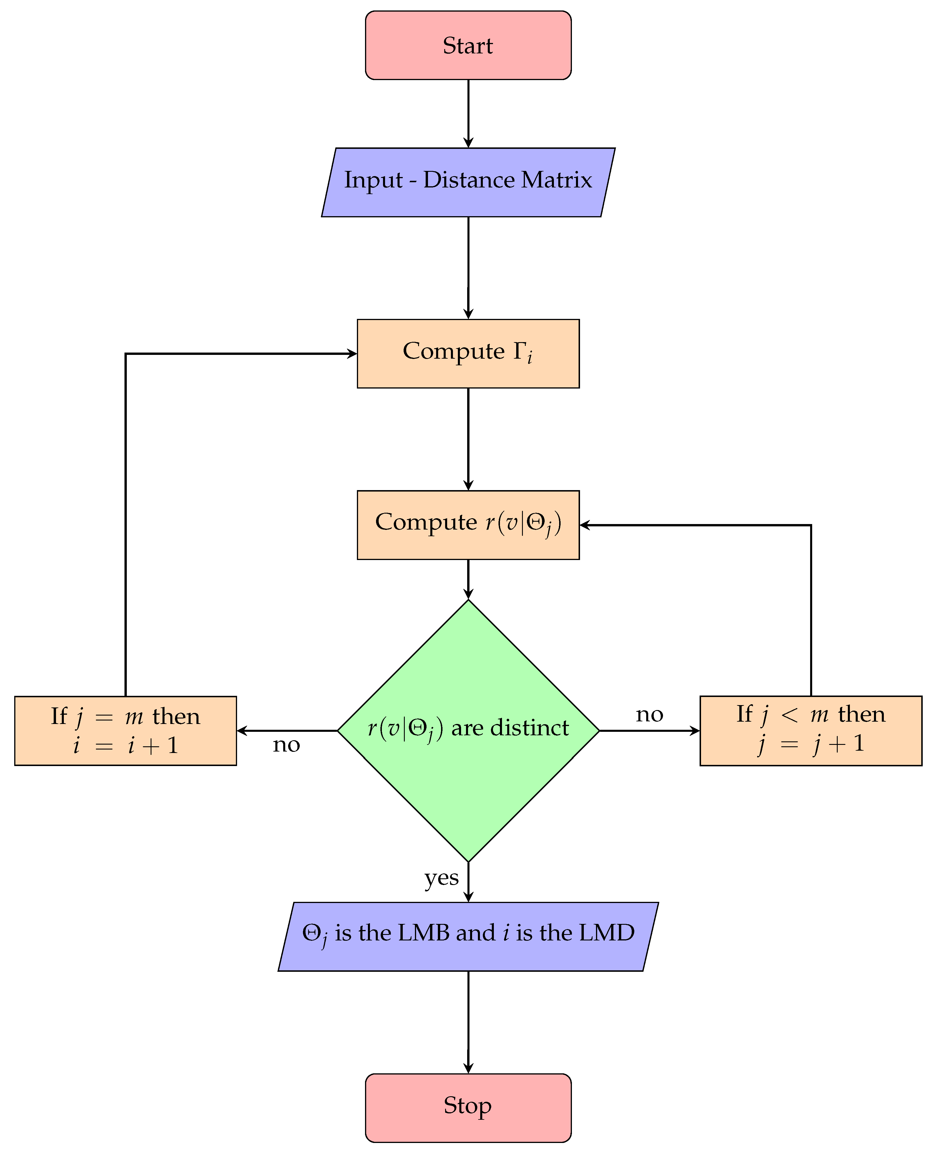
Let G be a connected graph having n number of nodes. The number of subsets of nodes is an exponential function, so as the value of n increases, Algorithm 1 may not give the answer in polynomial time, but for small sized problems, it will work. Figure 1 for Algorithm 1 given below will further clarify the computational procedure used to compute LMB and LMD.

Algorithm 1 Algorithm for the computation of LMB and LMD.

Require: $A=\left[a_{ij}\right]$      ▹$a_{ij}=1$ for adjacent nodes; otherwise, $a_{ij}=0$.    [STEP-1] Compute the distance matrix $D=\left[d_{ij}\right]$  ▹ where $d_{ij}$ is the distance between nodes $v_i$ and $v_j$.    [STEP-2] For $i=1$ to n         Compute ${\Gamma }_i=\{{\Theta }_1,{\Theta }_2,\dots ,{\Theta }_m\}$.            ▹ where each ${\Theta }_j$ is a subset of nodes containing i nodes and $m=\left(\genfrac{}{}{0pt}{}{n}{i}\right)$.    [STEP-3] For $j=1$ to m    Compute $r\left(v\right|{\Theta }_j)$ for each pair of adjacent nodes     if $r\left(v\right|{\Theta }_j)$ are distinct for each pair of adjacent nodes then        STOP     else        REPEAT STEP-3 with $j=j+1$     end if     if no ${\Theta }_j$ gives a distinct $r\left(v\right|{\Theta }_j)$ then        REPEAT STEP-2 with $i=i+1$     end if     [STEP-4] ${\Theta }_j$ is the LMB and i is the LMD.

3. Local Metric Dimension of Generalized Petersen Graphs

Coxeter introduced the generalized notion of Petersen graphs $P(n,k)$ in [29]. The node set $V\left(P(n,k)\right)=\{x_1,x_2,\dots ,x_n,y_1,y_2,\dots ,y_n\}$ and the edge set $E\left(P(n,k)\right)=\{x_i{x}_{i+k}:1\le i\le n\}\cup \{y_i{y}_{i+n}:1\le i\le n-1\}\cup \left\{y_n{y}_1\right\}\cup \{x_i{y}_i:1\le i\le n\}$, where $n\ge 3,1\le k\le \lfloor (n-1)/2\rfloor$ and subscripts are taken under modulo n. The nodes $x_i$ form the inner cycle, whereas nodes $y_i$ construct the outer cycle of these graphs.

3.1. LMD of $P(n,1)$

The current subsection computes the exact values of LMD of generalized Petersen graphs $P(n,1)$. Figure 2 below illustrates $P(6,1)$.

In the forthcoming result, we compute the LMD of $P(n,1)$.

Theorem 1.

Consider generalized Petersen graphs $P(n,1)$ with $n\ge 2$, then

$$di{m}_l\left(P(n,1)\right)=\left\{\begin{array}{ll}1,& \mathit{if}n\mathit{is}\mathit{even};\\ 2,& \mathit{if}n\mathit{is}\mathit{odd}.\end{array}\right.$$

Proof. 

The proof is split into two parts.

Case 1:

When n is even with $n=2\tau$ and $\tau \ge 1$ then $P(n,1)$ is a bipartite graph and Proposition 1 implies that $di{m}_l\left(P(n,1)\right)=1$ that is a set consisting of a single node would be the LMB.

Case 2:

When n is odd with $n=2\tau +1$ and $\tau \ge 1$.

For $\tau =1$, the set $\Theta =\{x_1,x_2\}$ with codes given below is LMG.

$r\left(x_1\right|\Theta )=(0,1),r\left(x_2\right|\Theta )=(1,0),r\left(x_3\right|\Theta )=(1,1),r\left(y_1\right|\Theta )=(1,2),r\left(y_2\right|\Theta )=(2,1),r\left(y_3\right|\Theta )=(2,2)$.

For $\tau \ge 2$, consider the subset $\Theta =\{x_1,x_2\}$ of $V\left(P\right(n,1\left)\right)$. The codes for all the nodes of $P(n,1)$ with respect to Θ are illustrated in

Table 1. Codes of nodes for $n=2\tau +1$ and $\tau \ge 2$.

Nodes	Codes
$x_{\varrho }$ ($\varrho =1$)	$(0,1)$
$x_{\varrho }$ ($\varrho =2$)	$(1,0)$
$x_{\varrho }$ ($3\le \varrho \le \tau +1$)	$(\varrho -1,\varrho -2)$
$x_{\varrho }$ ($\varrho =\tau +2$)	$(\tau ,\tau )$
$x_{\varrho }$ ($\tau +3\le \varrho \le n$)	$(n-\varrho +1,n-\varrho +2)$
$y_{\varrho }$ ($\varrho =1$)	$(1,2)$
$y_{\varrho }$ ($\varrho =2$)	$(2,1)$
$y_{\varrho }$ ($3\le \varrho \le \tau +1$)	$(\varrho ,\varrho -1)$
$y_{\varrho }$ ($\varrho =\tau +2$)	$(\tau +1,\tau +1)$
$y_{\varrho }$ ($\tau +3\le \varrho \le n$)	$(n-\varrho +2,n-\varrho +3)$

.

The codes above clearly specify that Θ is LMG; therefore, $di{m}_l(P(n,1)\le 2$. Hence, from Proposition 1, it can be inferred that $di{m}_l(P(n,1)=2$, as $P(n,1)$ is not a bipartite graph when n is odd. □

3.2. LMD of P(n, 2)

The current subsection computes the exact values of LMD of generalized Petersen graphs $P(n,2)$. Figure 3 below illustrates $P(6,2)$.

In the forthcoming results, we compute the LMD of $P(n,2)$.

Theorem 2.

Consider generalized Petersen graphs $P(n,2)$ with $n\ge 5$, then $di{m}_l\left(P(n,2)\right)\ge 3$ when $n=4\tau +1$ for $\tau =1$ and $\tau \ge 7$.

Proof. 

Suppose $di{m}_l\left(P(n,2)\right)=2$ such that $|\Theta |=2$ with $n=4\tau +1$ for $\tau =1$ and $\tau \ge 7$, then the possible cases of proof are given as follows.

Case 1:

When both nodes of Θ are from $x_i^{\prime }s$, we may assume that one of the two nodes is $x_1$ and the other is $x_{\varrho }$, where $2\le \varrho \le n$.

Case 1.1

When $\varrho =2t$, and $1\le t\le \tau$, then for $\tau =1$, $r\left(y_{2\tau +1}\right|\Theta )=(\tau +1,\tau +1)=r\left(y_{2\tau +2}\right|\Theta )$ and for $\tau \ge 7$, $r\left(y_{2\tau +1}\right|\Theta )=(\tau +1,\tau -t+2)=r\left(y_{2\tau +2}\right|\Theta )$, which is a contradictory fact.

Case 1.2

When $\varrho =2t$, and $\tau +1\le t\le 2\tau$, then for $\tau =1$, $r\left(y_{2\tau }\right|\Theta )=(\tau +1,\tau +1)=r\left(y_{2\tau +1}\right|\Theta )$ and for $\tau \ge 7$, $r\left(y_{2\tau }\right|\Theta )=(\tau +1,t-\tau +1)=r\left(y_{2\tau +1}\right|\Theta )$, which is a contradictory fact.

Case 1.3

When $\varrho =2t+1$. For $\tau =1$, $r\left(y_4\right|\Theta )=(\tau +1,\tau +1)=r\left(y_5\right|\Theta )$ when $\varrho =3$ and $r\left(y_3\right|\Theta )=(\tau +1,\tau +1)=r\left(y_4\right|\Theta )$ when $\varrho =5$.

For $\tau \ge 7$ and $1\le t\le \tau -1$, $r\left(y_{2\tau }\right|\Theta )=(\tau +1,\tau -t+1)=r\left(y_{2\tau +1}\right|\Theta )$, which is a contradictory fact for both subcases.

Case 1.4

When $\varrho =2t+1$. For $\tau \ge 7$ and $t=\tau$, $r\left(y_{2\tau +2}\right|\Theta )=(\tau +1,2)=r\left(y_{2\tau +3}\right|\Theta )$.

For $\tau \ge 7$ and $\tau +1\le t\le 2\tau$, $r\left(y_{2\tau +1}\right|\Theta )=(\tau +1,t-\tau +1)=r\left(y_{2\tau +2}\right|\Theta )$.

Case 2:

When both nodes of Θ are from $y_i^{\prime }s$. We may assume that one of the two nodes is $y_1$ and the other is $y_{\varrho }$, where $2\le \varrho \le n$.

Case 2.1

When $\varrho =2t$. For $\tau =1$ and $1\le t\le \tau$, $r\left(x_{2\tau +1}\right|\Theta )=(\tau +1,\tau +1)=r\left(x_{2\tau +3}\right|\Theta )$.

For $\tau \ge 7$ and $1\le t\le \tau -2$, $r\left(y_{2\tau +1}\right|\Theta )=(\tau +2,\tau -t+3)=r\left(y_{2\tau +2}\right|\Theta )$.

This is a contradictory fact in both subcases.

Case 2.2

When $\varrho =2t$. For $\tau =1$ and $\tau +1\le t\le 2\tau$, $r\left(x_{2\tau }\right|\Theta )=(\tau +1,\tau +1)=r\left(x_{2\tau +2}\right|\Theta )$.

For $\tau \ge 7$ and $\tau -1\le t\le 2\tau -4$, $r\left(y_{\tau -1}\right|\Theta )=(\tau -2,t-1)=r\left(y_{\tau }\right|\Theta )$.

For $\tau \ge 7$ and $\tau -3\le t\le 2\tau$, $r\left(y_{\tau -1}\right|\Theta )=(\tau -2,3\tau -t-1)=r\left(y_{\tau }\right|\Theta )$.

This is a contradictory fact in the above subcases.

Case 2.3

When $\varrho =2t+1$. For $\tau =1$ and $1\le t\le \tau$, $r\left(x_{2\tau }\right|\Theta )=(\tau +1,\tau +1)=r\left(x_{2\tau +2}\right|\Theta )$.

For $\tau \ge 7$ and $1\le t\le \tau -2$, $r\left(y_{2\tau +2}\right|\Theta )=(\tau +2,\tau -t+3)=r\left(y_{2\tau +3}\right|\Theta )$.

This is a contradictory fact in both subcases.

Case 2.4

When $\varrho =2t+1$. For $\tau \ge 7$ and $\tau -1\le t\le \tau +1$, $r\left(y_{3\tau +1}\right|\Theta )=(\tau -1,2\tau -t-1)=r\left(y_{3\tau +2}\right|\Theta )$.

For $\tau \ge 7$ and $t=\tau +2$, $r\left(y_{3\tau +3}\right|\Theta )=(\tau -2,\tau -2)=r\left(y_{3\tau +4}\right|\Theta )$.

For $\tau \ge 7$ and $\tau +3\le t\le 2\tau$, $r\left(y_{2\tau +1}\right|\Theta )=(\tau +2,t-\tau +2)=r\left(y_{2\tau +2}\right|\Theta )$.

Case 3:

When one of the nodes of Θ is from $x_i^{\prime }s$ and other from $y_i^{\prime }s$. We may assume that one of the two nodes is $x_1$ and the other is $y_{\varrho }$, where $1\le \varrho \le n$.

Case 3.1

When $\varrho =2t$. For $\tau =1$ and $1\le t\le \tau +1$, we have:

$r\left(y_4\right|\Theta )=(\tau +1,\tau +1)=r\left(y_5\right|\Theta )$ when $t=1$, $r\left(x_2\right|\Theta )=(\tau +1,\tau +1)=r\left(y_2\right|\Theta )$ when $t=2$,

For $\tau \ge 7$ and $1\le t\le \tau -2$, $r\left(y_{2\tau +1}\right|\Theta )=(\tau +1,\tau -t+3)=r\left(y_{2\tau +2}\right|\Theta )$.

This is a contradictory fact in the above subcases.

Case 3.2

When $\varrho =2t$.

For $\tau \ge 7$ and $\tau -1\le t\le 2\tau -4$, $r\left(y_{\tau -1}\right|\Theta )=(\tau -3,t-1)=r\left(y_{\tau }\right|\Theta )$.

For $\tau \ge 7$ and $2\tau -3\le t\le 2\tau$, $r\left(y_{\tau -1}\right|\Theta )=(\tau -3,3\tau -t-1)=r\left(y_{\tau }\right|\Theta )$.

This is a contradictory fact in the above subcases.

Case 3.3

When $\varrho =2t-1$. For $\tau =1$ and $1\le t\le 2\tau +1$ we have:

$r\left(y_3\right|\Theta )=(\tau +1,\tau +1)=r\left(y_4\right|\Theta )$ when $t=1$, $r\left(x_5\right|\Theta )=(\tau +1,\tau +1)=r\left(y_5\right|\Theta )$ when $t=2$, $r\left(y_2\right|\Theta )=(\tau +1,\tau +1)=r\left(y_3\right|\Theta )$ when $t=3$.

For $\tau \ge 7$ and $1\le t\le \tau -2$, $r\left(y_{2\tau }\right|\Theta )=(\tau +1,\tau -t+3)=r\left(y_{2\tau +1}\right|\Theta )$.

This is a contradictory fact in both subcases.

Case 3.4

When $\varrho =2t-1$. For $\tau \ge 7$ and $t=\tau -1$, $r\left(y_{4\tau }\right|\Theta )=(2,\tau +1)=r\left(y_{4\tau +1}\right|\Theta )$.

For $\tau \ge 7$ and $t=\tau$, $r\left(y_{4\tau }\right|\Theta )=(2,\tau +2)=r\left(y_{4\tau +1}\right|\Theta )$.

For $\tau \ge 7$ and $\tau +1\le t\le 2\tau -4$, $r\left(y_{4\tau }\right|\Theta )=(2,2\tau -t+3)=r\left(y_{4\tau +1}\right|\Theta )$. For $\tau \ge 7$ and $2\tau -3\le t\le 2\tau +1$, $r\left(y_{2\tau +1}\right|\Theta )=(\tau +1,t-\tau +1)=r\left(y_{2\tau +2}\right|\Theta )$.

The above cases prove our assertion that $di{m}_l\left(P(n,2)\right)\ge 3$ when $n=4\tau +1$ for $\tau =1$ and $\tau \ge 7$. □

Theorem 3.

Consider generalized Petersen graphs $P(n,2)$ with $n\ge 5$, then

$$di{m}_l\left(P(n,2)\right)=\left\{\begin{array}{ll}2,& \mathit{if}n=4\tau \mathit{for}\tau \ge 2;\\ 2,& \mathit{if}n=4\tau +2\mathit{for}\tau \ge 1;\\ 2,& \mathit{if}n=4\tau +3\mathit{for}\tau \ge 1;\\ 2,& \mathit{if}n=4\tau +1\mathit{for}\tau \in \{2,3,4,5,6\};\\ 3,& \mathit{if}n=4\tau +1\mathit{for}\tau =1\mathit{and}\tau \ge 7.\end{array}\right.$$

Proof. 

• Case 1: When $n=4\tau$ and $\tau \ge 2$, For $\tau =2,3,4,5$, it is easy to check that the sets $\{y_6,y_8\},\{y_{10},y_{12}\},\{y_9,y_{16}\},\{y_{12},y_{20}\}$ are the LMG.

For $\tau \ge 6$, consider the subset $\Theta =\{y_1,y_{2\tau -3}\}$ of $V\left(P\right(n,2\left)\right)$. The codes for all the nodes of $P(n,2)$ with respect to Θ are illustrated in

Table 2. Codes of nodes for $n=4\tau$ and $\tau \ge 6$.

Nodes	Codes
$x_{2\varrho -1}$ ($1\le \varrho \le \tau -1$)	$(\varrho ,\tau -\varrho )$
$x_{2\varrho }$ ($1\le \varrho \le \tau -2$)	$(\varrho +1,\tau -\varrho )$
$x_{2\varrho }$ ($\tau -1\le \varrho \le \tau$)	$(\varrho +1,\varrho -\tau +3)$
$x_{2\varrho -1}$ ($\tau \le \varrho \le \tau +1$)	$(\varrho ,\varrho -\tau +2)$
$x_{2\varrho }$ ($\tau +1\le \varrho \le 2\tau -2$)	$(2\tau -\varrho +2,\varrho -\tau +3)$
$x_{2\varrho -1}$ ($\tau +2\le \varrho \le 2\tau -1$)	$(2\tau -\varrho +2,\varrho -\tau +2)$
$x_{2\varrho }$ ($2\tau -1\le \varrho \le 2\tau$)	$(2\tau -\varrho +2,3\tau -\varrho )$
$x_{2\varrho -1}$ ($\varrho =2\tau$)	$(2,\tau )$
$y_{\varrho }$ ($\varrho =1$)	$(0,\tau )$
$y_{\varrho }$ ($\varrho =2$)	$(1,\tau )$
$y_{\varrho }$ ($\varrho =3$)	$(2,\tau -1)$
$y_{\varrho }$ ($\varrho =4$)	$(3,\tau -1)$
$y_{2\varrho +1}$ ($2\le \varrho \le \tau -4$)	$(\varrho +2,\tau -\varrho )$
$y_{2\varrho }$ ($3\le \varrho \le \tau -4,\tau \ge 7$)	$(\varrho +2,\tau -\varrho +1)$
$y_{2\varrho }$ ($\varrho =\tau -3$)	$(\tau -1,3)$
$y_{2\varrho +1}$ ($\varrho =\tau -3$)	$(\tau -1,2)$
$y_{2\varrho }$ ($\varrho =\tau -2$)	$(\tau ,1)$
$y_{2\varrho +1}$ ($\varrho =\tau -2$)	$(\tau ,0)$
$y_{2\varrho }$ ($\varrho =\tau -1$)	$(\tau +1,1)$
$y_{2\varrho +1}$ ($\varrho =\tau -1$)	$(\tau +1,2)$
$y_{2\varrho }$ ($\varrho =\tau$)	$(\tau +2,3)$
$y_{2\varrho +1}$ ($\tau \le \varrho \le 2\tau -2$)	$(2\tau -\varrho +2,\varrho -\tau +4)$
$y_{2\varrho }$ ($\tau +1\le \varrho \le 2\tau -2$)	$(2\tau -\varrho +3,\varrho -\tau +4)$
$y_{2\varrho }$ ($\varrho =2\tau -1$)	$(3,\tau +2)$
$y_{2\varrho +1}$ ($\varrho =2\tau -1$)	$(2,\tau +1)$
$y_{2\varrho }$ ($\varrho =2\tau$)	$(1,\tau +1)$

.

• Case 2: When $n=4\tau +2$ and $\tau \ge 1$. Consider the subset $\Theta =\{x_1,x_2\}$ of $V\left(P\right(n,2\left)\right)$. For $\tau =1,2,3,4,5$, it is easy to check that Θ is a LMG. For $\tau \ge 6$, the codes for all the nodes of $P(n,2)$ with respect to Θ are illustrated in

  Table 3. Codes of nodes for $n=4\tau +2$ and $\tau \ge 6$.

  Nodes	Codes
  $x_{\varrho }$ ($\varrho =1$)	$(0,3)$
  $x_{\varrho }$ ($\varrho =2$)	$(3,0)$
  $x_{2\varrho +1}$ ($1\le \varrho \le \tau$)	$(\varrho ,\varrho +2)$
  $x_{2\varrho }$ ($2\le \varrho \le \tau +1$)	$(\varrho +2,\varrho -1)$
  $x_{2\varrho +1}$ ($\tau +1\le \varrho \le 2\tau$)	$(2\tau -\varrho +1,2\tau -\varrho +4)$
  $x_{2\varrho }$ ($\tau +2\le \varrho \le 2\tau +1$)	$(2\tau -\varrho +4,2\tau -\varrho +2)$
  $y_{\varrho }$ ($\varrho =1$)	$(1,2)$
  $y_{2\varrho +1}$ ($1\le \varrho \le \tau$)	$(\varrho +1,\varrho +1)$
  $y_{2\varrho }$ ($1\le \varrho \le \tau +1$)	$(\varrho +1,\varrho )$
  $y_{2\varrho +1}$ ($\tau +1\le \varrho \le 2\tau$)	$(2\tau -\varrho +2,2\tau -\varrho +3)$
  $y_{2\varrho }$ ($\tau +2\le \varrho \le 2\tau +1$)	$(2\tau -\varrho +3,2\tau -\varrho +3)$

  .
• Case 3: When $n=4\tau +3$ and $\tau \ge 1$. Consider the subset $\Theta =\{x_1,x_2\}$ of $V\left(P\right(n,2\left)\right)$. For $\tau =1,2$, it is easy to check that Θ is a LMG. For $\tau \ge 3$, the codes for all the nodes of $P(n,2)$ with respect to Θ are illustrated in

  Table 4. Codes of nodes for $n=4\tau +3$ and $\tau \ge 3$.

  Nodes	Codes
  $x_{\varrho }$ ($\varrho =1$)	$(0,3)$
  $x_{\varrho }$ ($\varrho =2$)	$(3,0)$
  $x_{2\varrho +1}$ ($1\le \varrho \le \tau$)	$(\varrho ,\varrho +2)$
  $x_{2\varrho }$ ($2\le \varrho \le \tau$)	$(\varrho +2,\varrho -1)$
  $x_{2\varrho }$ ($\tau +1\le \varrho \le \tau +3$)	$(2\tau -\varrho +2,\varrho -1)$
  $x_{2\varrho }$ ($\tau +4\le \varrho \le 2\tau +1$)	$(2\tau -\varrho +2,2\tau -\varrho +5)$
  $x_{2\varrho +1}$ ($\varrho =\tau +1$)	$(\tau +1,\tau +1)$
  $x_{2\varrho +1}$ ($\tau +2\le \varrho \le 2\tau +1$)	$(2\tau -\varrho +4,2\tau -\varrho +2)$
  $y_{\varrho }$ ($\varrho =1$)	$(1,2)$
  $y_{2\varrho }$ ($1\le \varrho \le \tau +1$)	$(\varrho +1,\varrho )$
  $y_{2\varrho +1}$ ($1\le \varrho \le \tau +1$)	$(\varrho +1,\varrho +1)$
  $y_{2\varrho }$ ($\tau +2\le \varrho \le 2\tau +1$)	$(2\tau -\varrho +3,2\tau -\varrho +4)$
  $y_{2\varrho +1}$ ($\tau +2\le \varrho \le 2\tau +1$)	$(2\tau -\varrho +3,2\tau -\varrho +3)$

  .
• Case 4: When $n=4\tau +1$ and $\tau \ge 1$. For $\tau =2,3,4,5,6$, it is easy to check that the sets $\{y_1,y_3\},\{y_1,y_4\},\{y_1,y_8\},\{y_1,y_8\},\{y_1,y_{10}\}$ are LMG.

For $\tau =1$ and $\tau \ge 7$, consider the subset $\Theta =\{x_1,x_2,x_{2\tau +2}\}$ of $V\left(P\right(n,2\left)\right)$. For $\tau =1$, it is easy to check that $\Theta =\{x_1,x_2,x_4\}$ is a LMG. The codes for all the nodes of $P(n,2)$ with respect to Θ for $\tau \ge 7$ are illustrated in

Table 5. Codes of nodes for $n=4\tau +1$ and $\tau \ge 7$.

Nodes	Codes
$x_{\varrho }$ ($\varrho =1$)	$(0,3,\tau )$
$x_{\varrho }$ ($\varrho =2$)	$(3,0,\tau )$
$x_{\varrho }$ ($\varrho =3$)	$(1,3,\tau +1)$
$x_{2\varrho }$ ($2\le \varrho \le \tau -1$)	$(\varrho +2,\varrho -1,\tau -\varrho +1)$
$x_{2\varrho +1}$ ($2\le \varrho \le \tau -1$)	$(\varrho ,\varrho +2,\tau -\varrho +3)$
$x_{2\varrho }$ ($\varrho =\tau$)	$(\tau +1,\tau -1,1)$
$x_{2\varrho +1}$ ($\varrho =\tau$)	$(\tau ,\tau +1,3)$
$x_{2\varrho }$ ($\varrho =\tau +1$)	$(\tau ,\tau ,0)$
$x_{2\varrho +1}$ ($\varrho =\tau +1$)	$(\tau +1,\tau ,3)$
$x_{2\varrho }$ ($\varrho =\tau +2$)	$(\tau -1,\tau +1,1)$
$x_{2\varrho +1}$ ($\tau +2\le \varrho \le 2\tau -1$)	$(2\tau -\varrho +3,2\tau -\varrho +1,\varrho -\tau +2)$
$x_{2\varrho }$ ($\tau +3\le \varrho \le 2\tau$)	$(2\tau -\varrho +1,2\tau -\varrho +4,\varrho -\tau -1)$
$x_{2\varrho +1}$ ($\varrho =2\tau$)	$(3,1,\tau +1)$
$y_{\varrho }$ ($\varrho =1$)	$(1,2,\tau +1)$
$y_{2\varrho }$ ($1\le \varrho \le \tau$)	$(\varrho +1,\varrho ,\tau -\varrho +2)$
$y_{2\varrho +1}$ ($1\le \varrho \le \tau$)	$(\varrho +1,\varrho +1,\tau -\varrho +2)$
$y_{2\varrho }$ ($\varrho =\tau +1$)	$(\tau +1,\tau +1,1)$
$y_{2\varrho +1}$ ($\tau +1\le \varrho \le 2\tau$)	$(2\tau -\varrho +2,2\tau -\varrho +2,\varrho -\tau +1)$
$y_{2\varrho }$ ($\tau +2\le \varrho \le 2\tau$)	$(2\tau -\varrho +2,2\tau -\varrho +3,\varrho -\tau )$

.

The codes in the above cases clearly specify that Θ is LMG and, as $\left(P\right(n,2)$ is not a bipartite graph, both Proposition 1 and Theorem 2 prove our assertion. □

Example 1:

To illustrate how the codes of nodes can be generated, we consider an example of $P(24,2)$. Here, $n=4\tau$ and $\tau =6$. Now, the codes for all the nodes can be generated from Table 2. The codes for all the nodes of $P(24,2)$ are given in

Table 6. Codes of nodes for $P(24,2)$.

Codes	Codes	Codes	Codes
$x_1(1,5)$	$y_1(0,6)$	$x_{13}(7,3)$	$y_{13}(8,4)$
$x_2(2,5)$	$y_2(1,6)$	$x_{14}(7,4)$	$y_{14}(8,5)$
$x_3(2,4)$	$y_3(2,5)$	$x_{15}(6,4)$	$y_{15}(7,5)$
$x_4(3,4)$	$y_4(3,5)$	$x_{16}(6,5)$	$y_{16}(7,6)$
$x_5(3,3)$	$y_5(4,4)$	$x_{17}(5,5)$	$y_{17}(6,6)$
$x_6(4,3)$	$y_6(5,3)$	$x_{18}(5,6)$	$y_{18}(6,7)$
$x_7(4,2)$	$y_7(5,2)$	$x_{19}(4,6)$	$y_{19}(5,7)$
$x_8(5,2)$	$y_8(6,1)$	$x_{20}(4,7)$	$y_{20}(5,8)$
$x_9(5,1)$	$y_9(6,0)$	$x_{21}(3,7)$	$y_{21}(4,8)$
$x_{10}(6,2)$	$y_{10}(7,1)$	$x_{22}(3,7)$	$y_{22}(3,8)$
$x_{11}(6,2)$	$y_{11}(7,2)$	$x_{23}(2,6)$	$y_{23}(2,7)$
$x_{12}(7,3)$	$y_{12}(8,3)$	$x_{24}(2,6)$	$y_{24}(1,7)$

.

We can easily check from these codes that each pair of adjacent nodes has distinct codes.

3.3. LMD of P(n, 3)

The current subsection computes the exact values of LMD of $P(n,3)$ graphs. Figure 4 below illustrates $P(8,3)$.

In the forthcoming result, we compute the LMD of $P(n,3)$ graphs.

Theorem 4.

Consider generalized Petersen graphs $P(n,3)$ with $n\ge 7$, then

$$di{m}_l\left(P(n,3)\right)=\left\{\begin{array}{ll}1,& \mathit{if}n\mathit{is}\mathit{even};\\ 2,& \mathit{if}n\mathit{is}\mathit{odd}.\end{array}\right.$$

Proof. 

The proof is split into two parts.

• Case 1: When n is even, then $P(n,3)$ is a bipartite graph and Proposition 1 implies that $di{m}_l\left(P(n,3)\right)=1$, which is a set consisting of a single node, would be the LMB.
• Case 2: When n is odd, then there are three subcases.
• Case 2a: When $n=6\tau +1$ and $\tau \ge 1$. For $\tau =1$, it can verified easily that the set $\{x_1,y_3\}$ is a LMG. For $\tau =2,3,4$, it can also be verified easily that the set $\{x_1,x_4\}$ is a LMG.

For $\tau \ge 5$, consider the subset $\Theta =\{x_1,x_4\}$ of $V\left(P\right(n,3\left)\right)$. The codes for all the nodes of $P(n,3)$ with respect to Θ are illustrated in

Table 7. Codes of nodes for $n=6\tau +1$ and $\tau \ge 5$.

Nodes	Codes
$x_{\varrho }$ ($\varrho =1$)	$(0,1)$
$x_{\varrho }$ ($\varrho =2$)	$(3,4)$
$x_{\varrho }$ ($\varrho =3$)	$(4,3)$
$x_{\varrho }$ ($\varrho =4$)	$(1,0)$
$x_{3\varrho +2}$ ($1\le \varrho \le \tau -2$)	$(\varrho +3,\varrho +2)$
$x_{3\varrho }$ ($2\le \varrho \le \tau -1$)	$(\varrho +3,\varrho +2)$
$x_{3\varrho +1}$ ($2\le \varrho \le \tau +1$)	$(\varrho ,\varrho -1)$
$x_{2\varrho +1}$ ($\varrho =\tau$)	$(\tau ,\tau +1,3)$
$x_{2\varrho }$ ($\varrho =\tau +1$)	$(\tau ,\tau ,0)$
$x_{2\varrho +1}$ ($\varrho =\tau +1$)	$(\tau +1,\tau ,3)$
$x_{2\varrho }$ ($\varrho =\tau +2$)	$(\tau -1,\tau +1,1)$
$x_{2\varrho +1}$ ($\tau +2\le \varrho \le 2\tau -1$)	$(2\tau -\varrho +3,2\tau -\varrho +1,\varrho -\tau +2)$
$x_{2\varrho }$ ($\tau +3\le \varrho \le 2\tau$)	$(2\tau -\varrho +1,2\tau -\varrho +4,\varrho -\tau -1)$
$x_{2\varrho +1}$ ($\varrho =2\tau$)	$(3,1,\tau +1)$
$y_{\varrho }$ ($\varrho =1$)	$(1,2,\tau +1)$
$y_{2\varrho }$ ($1\le \varrho \le \tau$)	$(\varrho +1,\varrho ,\tau -\varrho +2)$
$y_{2\varrho +1}$ ($1\le \varrho \le \tau$)	$(\varrho +1,\varrho +1,\tau -\varrho +2)$
$y_{2\varrho }$ ($\varrho =\tau +1$)	$(\tau +1,\tau +1,1)$
$y_{2\varrho +1}$ ($\tau +1\le \varrho \le 2\tau$)	$(2\tau -\varrho +2,2\tau -\varrho +2,\varrho -\tau +1)$
$y_{2\varrho }$ ($\tau +2\le \varrho \le 2\tau$)	$(2\tau -\varrho +2,2\tau -\varrho +3,\varrho -\tau )$

.

• Case 2b: When $n=6\tau +3$ and $\tau \ge 1$. For $\tau =1,2,3,4$, it can verified easily that the set $\{x_1,x_4\}$ is a LMG.

For $\tau \ge 5$, consider the subset $\Theta =\{x_1,x_4\}$ of $V\left(P\right(n,3\left)\right)$. The codes for all the nodes of $P(n,3)$ with respect to Θ are illustrated in

Table 8. Codes of nodes for $n=6\tau +3$ and $\tau \ge 5$.

Nodes	Codes
$x_{\varrho }$ ($\varrho =1$)	$(0,1)$
$x_{\varrho }$ ($\varrho =2$)	$(3,4)$
$x_{\varrho }$ ($\varrho =3$)	$(4,3)$
$x_{\varrho }$ ($\varrho =4$)	$(1,0)$
$x_{3\varrho +2}$ ($1\le \varrho \le \tau$)	$(\varrho +3,\varrho +2)$
$x_{3\varrho }$ ($2\le \varrho \le \tau$)	$(\varrho +3,\varrho +2)$
$x_{3\varrho +1}$ ($2\le \varrho \le \tau$)	$(\varrho ,\varrho -1)$
$x_{3\varrho }$ ($\varrho =\tau +1$)	$(\tau +3,\tau +3)$
$x_{3\varrho +1}$ ($\varrho =\tau +1$)	$(\tau ,\tau )$
$x_{3\varrho +2}$ ($\varrho =\tau +1$)	$(\tau +3,\tau +3)$
$x_{3\varrho }$ ($\tau +2\le \varrho =2\tau +1$)	$(2\tau -\varrho +4,2\tau -\varrho +5)$
$x_{3\varrho +1}$ ($\tau +2\le \varrho \le 2\tau$)	$(2\tau -\varrho +1,2\tau -\varrho +2)$
$x_{3\varrho +2}$ ($\tau +2\le \varrho \le 2\tau$)	$(2\tau -\varrho +4,2\tau -\varrho +5)$
$y_{\varrho }$ ($\varrho =1$)	$(1,2)$
$y_{\varrho }$ ($\varrho =2$)	$(2,3)$
$y_{3\varrho }$ ($1\le \varrho \le \tau$)	$(\varrho +2,\varrho +1)$
$y_{3\varrho +1}$ ($1\le \varrho \le \tau$)	$(\varrho +1,\varrho )$
$y_{3\varrho +2}$ ($1\le \varrho \le \tau$)	$(\varrho +2,\varrho +1)$
$y_{3\varrho }$ ($\varrho =\tau +1$)	$(\tau +2,\tau +2)$
$y_{3\varrho +1}$ ($\varrho =\tau +1$)	$(\tau +1,\tau +1)$
$y_{3\varrho +2}$ ($\varrho =\tau +1$)	$(\tau +2,\tau +2)$
$y_{3\varrho }$ ($\tau +2\le \varrho \le 2\tau +1$)	$(2\tau -\varrho +3,2\tau -\varrho +4)$
$y_{3\varrho +1}$ ($\tau +2\le \varrho \le 2\tau$)	$(2\tau -\varrho +2,2\tau -\varrho +3)$
$y_{3\varrho +2}$ ($\tau +2\le \varrho \le 2\tau$)	$(2\tau -\varrho +3,2\tau -\varrho +4)$

.

• Case 2c: When $n=6\tau +5$ and $\tau \ge 1$. For $\tau =1,2,3$, it can verified easily that the set $\{x_1,x_4\}$ is a LMG.

For $\tau \ge 4$, consider the subset $\Theta =\{x_1,x_4\}$ of $V\left(P\right(n,3\left)\right)$. The codes for all the nodes of $P(n,3)$ with respect to Θ are illustrated in

Table 9. Codes of nodes for $n=6\tau +5$ and $\tau \ge 4$.

Nodes	Codes
$x_{\varrho }$ ($\varrho =1$)	$(0,1)$
$x_{\varrho }$ ($\varrho =2$)	$(3,4)$
$x_{3\varrho }$ ($1\le \varrho \le \tau -1$)	$(\varrho +3,\varrho +2)$
$x_{3\varrho +2}$ ($1\le \varrho \le \tau$)	$(\varrho +3,\varrho +2)$
$x_{3\varrho +1}$ ($2\le \varrho \le \tau +2$)	$(\varrho ,\varrho -1)$
$x_{3\varrho }$ ($\varrho =\tau$)	$(\tau +2,\tau +2)$
$x_{3\varrho }$ ($\tau +2\le \varrho \le 2\tau +1$)	$(2\tau -\varrho +2,2\tau -\varrho +3)$
$x_{3\varrho +2}$ ($\varrho =\tau +1$)	$(\tau +3,\tau +3)$
$x_{3\varrho +2}$ ($\tau +2\le \varrho \le 2\tau +1$)	$(2\tau -\varrho +4,2\tau -\varrho +5)$
$x_{3\varrho +1}$ ($\varrho =\tau +3$)	$(\tau +2,\tau +2)$
$x_{3\varrho +1}$ ($\tau +4\le \varrho \le 2\tau +1$)	$(2\tau -\varrho +5,2\tau -\varrho +6)$
$y_{\varrho }$ ($\varrho =1$)	$(1,2)$
$y_{\varrho }$ ($\varrho =2$)	$(2,3)$
$y_{3\varrho }$ ($1\le \varrho \le \tau$)	$(\varrho +2,\varrho +1)$
$y_{3\varrho +1}$ ($1\le \varrho \le \tau +1$)	$(\varrho +1,\varrho )$
$y_{3\varrho +2}$ ($1\le \varrho \le \tau$)	$(\varrho +2,\varrho +1)$
$y_{3\varrho }$ ($\varrho =\tau +1$)	$(\tau +2,\tau +2)$
$y_{3\varrho +2}$ ($\varrho =\tau +1$)	$(\tau +2,\tau +2)$
$y_{3\varrho +2}$ ($\varrho =\tau +1$)	$(\tau +2,\tau +2)$
$y_{3\varrho }$ ($\tau +2\le \varrho \le 2\tau +1$)	$(2\tau -\varrho +3,2\tau -\varrho +4)$
$y_{3\varrho +1}$ ($\varrho =\tau +2$)	$(\tau +2,\tau +2)$
$y_{3\varrho +2}$ ($\tau +2\le \varrho \le 2\tau +1$)	$(2\tau -\varrho +3,2\tau -\varrho +4)$
$y_{3\varrho +1}$ ($\tau +3\le \varrho \le 2\tau +1$)	$(2\tau -\varrho +4,2\tau -\varrho +5)$

.

The codes above clearly specify that Θ is LMG; therefore, $di{m}_l(P(n,3)\le 2$. Hence, from Proposition 1, it can be inferred that $di{m}_l(P(n,3)=2$, as $P(n,3)$ is not a bipartite graph when n is odd. □

4. Applications of Local Metric Basis

We extend this study by applying LMB in the optimal placement of facilities like hospitals, fire stations, and grocery stores in a locality. The objective is to access these facilities in optimal time, which can be converted into a graph theory problem if we assume different regions as nodes connected by edges where the length of each edge gives the average distance between two regions. For further explanation, we give an example.

Example 2.

Consider a locality in which different regions are in the form of a $P(6,2)$ graph as shown in Figure 3. The LMB is the set $\{x_1,x_2\}$ which contains the smallest number of nodes such that each pair of adjacent nodes gets different codes. Here, we can construct facilities like grocery stores at nodes $x_1$ and $x_2$. The codes are $x_1(0,3),x_2(3,0),x_3(1,3),x_4(4,1)$, $x_5(1,4),x_6(3,1),y_1(1,2),y_2(2,1),y_3(2,2),y_4(3,2),y_5(2,3),y_6(2,2)$. The codes of each node clearly identify the closest facility. The distinct codes of adjacent nodes help to use each facility optimally. The same codes for non-adjacent nodes indicate the alternate solutions and help to keep the code length shorter.

5. Conclusions

In this manuscript, we infer that the LMD of the generalized Petersen graphs $P(n,1),P(n,2)$, and $P(n,3)$ is constant and does not depend on the number of nodes in these families. The applications of LMB can be realized in identifying the optimal location for different facilities in an area. The prior knowledge of LMB of certain graphs, which can be distributed systems, would help in improving these systems. The algorithm proposed in the manuscript can be used to compute other versions of LMB for different families of graphs with minor modifications.

Open Problem 1. Compute the LMD of generalized Petersen graphs $P(n,k)$ for different values of n and k.

References

1. Slater, P.J. Leaves of Trees. In Proceedings of the 6th Southeastern Conference Combinatorics, Graph Theory and Computing, Congressus Numerantium, Boca Raton, FL, USA, 17–20 February 1975; Volume 14, pp. 549–559. [Google Scholar]
2. Harary, F.; Melter, R.A. On the metric dimension of a graph. Theory Comput. Syst. Ars Comb. 1976, 2, 191–195. [Google Scholar]
3. Khuller, S.; Raghavachari, B.; Rosenfeld, A. Landmarks in graphs. Discret. Appl. Math. 1996, 70, 217–229. [Google Scholar] [CrossRef]
4. Shao, Z.; Wu, P.; Zhu, E.; Chen, L. On metric dimension in some hex derived networks. Sensors 2019, 19, 94. [Google Scholar] [CrossRef] [PubMed]
5. Chartrand, G.; Eroh, L.; Johnson, M.A.; Oellermann, O.R. Resolvability in graphs and the metric dimension of a graph. Discret. Appl. Math. 2000, 105, 99–113. [Google Scholar] [CrossRef]
6. Sebö, A.; Tannier, E. On metric generators of graphs. Math. Oper. Res. 2004, 29, 383–393. [Google Scholar] [CrossRef]
7. Okamoto, F.; Crosse, L.; Phinezy, B.; Zhang, P.; Kalamazoo. The local metric dimension of a graph. Math. Bohem. 2010, 135, 239–255. [Google Scholar] [CrossRef]
8. Jothi, M.A.; Sankar, K. On the metric dimension of bipartite graphs. AKCE Int. J. Graphs Comb. 2023, 20, 287–290. [Google Scholar] [CrossRef]
9. Khan, A.; Haidar, G.; Abbas, N.; Khan, M.U.I.; Niazi, A.U.K.; Khan, A.U.I. Metric dimensions of bicyclic graphs. Mathematics 2023, 11, 869. [Google Scholar] [CrossRef]
10. Knor, M.; Skrekovski, R.; Vetrík, T. Metric dimension of circulant graphs with 5 consecutive generators. Mathematics 2024, 12, 1384. [Google Scholar] [CrossRef]
11. Sharma, S.K.; Bhat, V.K. Metric dimensions of heptagonal circular ladder. Discret. Math. Algorithms Appl. 2020, 13, 2050095. [Google Scholar] [CrossRef]
12. Zhang, C.; Haidar, G.; Khan, M.U.I.; Yousafzai, F.; Hila, K.; Khan, A.U.I. Constant time calculation of the metric dimension of the join of path graphs. Symmetry 2023, 15, 708. [Google Scholar] [CrossRef]
13. Klavžar, S.; Tavakoli, M. Local metric dimension of graphs: Generalized hierarchical products and some applications. Appl. Math. Comput. 2020, 364, 124676. [Google Scholar]
14. Yang, C.; Deng, X.A.; Liang, J.; Liu, Y. On the local metric dimension of graphs. J. Interconnect. Netw. 2024, 2350033. [Google Scholar] [CrossRef]
15. Abrishami, G.; Henning, M.A.; Tavakoli, M. Local metric dimension for graphs with small clique numbers. Discret. Math. 2022, 345, 112763. [Google Scholar] [CrossRef]
16. Lal, S.; Bhat, V.K. On the local metric dimension of generalized wheel graph. Asian-Eur. J. Math. 2023, 16, 2350194. [Google Scholar] [CrossRef]
17. Barragán-Ramírez, G.A.; Estrada-Moreno, A.; Ramírez-curz, Y. The Local Metric dimension of the lexicographic product of graphs. Bull. Malays. Math. Sci. Soc. 2019, 42, 2481–2496. [Google Scholar] [CrossRef]
18. Cahyabudi, A.N.; Kusmayadi, T.A. On the local metric dimension of a lollipop graph, a web graph and a friendship graph. J. Phys. Conf. Ser. 2017, 909, 012039. [Google Scholar] [CrossRef]
19. Listiana, Y.; Susilowati, L.; Slamin, S.; Osaye, F.J. A central local metric dimension on acyclic and grid graph. Aims Math. 2023, 8, 21298–21311. [Google Scholar] [CrossRef]
20. Pratama, J.A.B.Y.; Kusmayadi, T.A. On the local metric dimension of dipyramidal graph and king graph. AIP Conf. Proc. 2021, 2326, 020018. [Google Scholar]
21. Kelenc, A.; Kuziak, D.; Taranenko, A.; Yero, I.G. Mixed metric dimension of graph. Appl. Math. Comput. 2017, 314, 429–438. [Google Scholar]
22. Ramírez-Cruz, Y.; Oellermann, O.R.; Rodríguez-Velázquez, J.A. The simultaneous metric dimension of graph families. Discret. Appl. Math. 2016, 198, 241–250. [Google Scholar] [CrossRef]
23. Yero, I.G.; Estrado-Moreno, A.; Rodríguez-Velázquez, J.A. Computing the k-metric dimension of graphs. Appl. Math. Comput. 2017, 300, 60–69. [Google Scholar] [CrossRef]
24. Ahmad, S.; Chaudhry, M.A.; Javaid, I.; Salman, M. On the metric dimension of generalized Petersen graphs. Quaest. Math. 2013, 36, 421–435. [Google Scholar] [CrossRef]
25. Imran, M.; Baig, A.Q.; Shafiq, M.K.; Tomescu, I. On metric dimension of generalized Petersen graphs P(n, 3). Ars Comb. 2014, 117, 113–130. [Google Scholar]
26. Imran, M.; Siddiqui, M.K.; Naeem, R. On the metric dimension of generalized Petersen multigraphs. IEEE Access 2018, 6, 74328–74338. [Google Scholar] [CrossRef]
27. Javaid, I.; Ahmad, S.; Azhar, M.N. On the metric dimension of generalized Petersen graphs. Ars Comb. 2012, 105, 171–182. [Google Scholar]
28. Barragán-Ramírez, G.A.; Rodríguez-Velázquez, J.A. The local metric dimension of strong product graphs. Graphs Comb. 2016, 32, 1263–1278. [Google Scholar] [CrossRef]
29. Coxeter, H.S.M. Self-dual configurations and regular graphs. Bull. Am. Math. Soc. 1950, 56, 413–455. [Google Scholar] [CrossRef]
Figure 1. Flowchart for Algorithm 1.
Mathematics 12 02179 g001
Figure 2. P ( 6 , 1 ) .
Mathematics 12 02179 g002
Figure 3. P ( 6 , 2 ) .
Mathematics 12 02179 g003
Figure 4. P ( 8 , 3 ) .
Mathematics 12 02179 g004