Adaptive Neural Network Prescribed Time Control for Constrained Multi-Robotics Systems with Parametric Uncertainties

Abstract

This study designed an adaptive neural network (NN) control method for a category of multi-robotic systems with parametric uncertainties. In practical engineering applications, systems commonly face design challenges due to uncertainties in their parameters. Especially when a system’s parameters are completely unknown, the unpredictability caused by parametric uncertainties may increase control complexity, and even cause system instability. To address these problems, an adaptive NN compensation mechanism is proposed. Moreover, using backstepping and barrier Lyapunov functions (BLFs), guarantee that state constraints can be ensured. With the aid of the transform function, systems’ convergence speeds were greatly improved. Under the implemented control strategy, the prescribed time control of multi-robotic systems with parametric uncertainties under the prescribed performance was achieved. Finally, the efficacy of the proposed control strategy was verified through the application of several cases.

1. Introduction

Multi-robotic systems have extensive applications across various domains [1,2,3,4,5,6,7,8,9], including agriculture [10], healthcare [11], manufacturing automation [12,13], and other fields. In multi-robotic systems, cooperative control primarily includes consensus, formation, and containment control. Consensus control, considered the fundamental basis for cooperative control in multi-robotic systems, has captured the attention and interest of scholars [14,15,16]. In [5], the authors tackled the problem of adapting to changes in robot types within multi-robotic systems by introducing a collaborative relationship meta reinforcement learning method, which emphasizes inter-robot relationships to enhance performance. The authors in [15] introduced an echo control strategy to tackle multiagent consensus issues with interaction distortions. By having agents relay information back to neighbors, this approach forms a negative feedback loop, ensuring stability and convergence. In [17], the authors directed attention to addressing the consensus control problem within state-constrained nonlinear strict-feedback systems, introducing a pioneering distributed fuzzy optimal control approach to resolve it. For second-order nonlinear multiagent systems, the lag consensus problem was solved in [18]. As shown in [19], the authors tackled control issues related to consensus attainment in higher-order multi-agent systems, considering both leaderless and leader–follower disturbances. Note that it is necessary to consider the characteristics of convergence time while reaching systems consensus.

Many practical systems have requirements for convergence time, convergence process, and convergence accuracy. Prescribed time control methods [20,21,22,23,24] were suggested to secure system convergence within the prescribed time, irrespective of initial state and controller parameter. In [22], a novel distributed controller was proposed, utilizing time-varying control gains and a state transformation to achieve this objective. The focus of the author in [25] laid in event-triggered control methods for attaining prescribed-time bipartite consensus in first-order multiagent systems. They introduced efficient control laws and conditions, while also preventing Zeno behavior. Based on a distributed observer approach, a prescribed time observer-based controller for multiagent systems was proposed in [26]. The above studies all achieved the goal of enforcing systems to object states, and the convergence time remained preset, irrespective of these systems’ initial conditions. However, in the process of rapid convergence, a system’s state may significantly change, which may affect the system’s performance. How to guarantee the fast convergence of systems while guaranteeing the systems’ performance is still a problem worth discussing.

Systems uncertainty is a common situation that can lead to a significant degradation of control performance and may even affect the stability of the systems [27,28]. To end it, many scholars have conducted extensive research on uncertain systems [29,30,31]. NN is a promising tool for unknown uncertainty because of its out of the ordinary approximation ability. In [29], a novel wavelet-TSK-type fuzzy cerebellar model neural network was proposed for uncertain nonlinear systems. This neural network combines a cerebellar model neural network framework with a wavelet-function-based Takagi–Sugeno–Kang fuzzy inference model, offering enhanced effectiveness in handling system uncertainty. The author in [32] proposed a pioneering strategy integrating an NN controller within the approximate domain, providing a novel solution for global tracking control in uncertain nonlinear systems with output feedback. To address uncertainties in nonlinear systems, a novel adaptive event-triggered control strategy was proposed in [33]. The above studies have effectively addressed uncertainty within systems. However, when facing entirely unknown parameters, the application of an NN to handle this problem remains a topic for discussion.

In practical applications, with increasing demands for safety performance, the issue of handling state constraints has gained increasing attention in recent times [34,35,36]. The use of BLFs has emerged as an effective strategy to restrict tracking errors within predetermined ranges [37,38]. The authors in [35] introduced an innovative backstepping controller for hydraulic systems, incorporating extended state observers (ESOs) and an adaptive law to address uncertainties. The controller combines prescribed performance function (PPF) and barrier Lyapunov function (BLF) synthesis to address specified performance tracking. For a class of chained nonholonomic systems with full-state constraints, the author in [39] proposed a systematic strategy for the tracking controller based on BLFs. Further, considering full-state constraints and actuator failures, by incorporating BLFs and the backstepping technique, the author proposed an adaptive consensus control approach in [40]. It is noteworthy that the mentioned authors successfully addressed the issue of rapid changes in systems convergence by introducing BLFs. Therefore, the effectiveness of BLFs in solving constraint problems has been demonstrated, and were utilized in this study.

The key contributions of this study are summarized as follows:

• To achieve the balance between rapid convergence and systems performance, a transform function was constructed, integrating the speed function into the prescribed performance function. In addition, employing this method, which merges the proposed transformation function with BLFs at every step, guarantees that all errors of the systems converge to prescribed regions during the prescribed time. Simultaneously, it effectively prevents violations of state constraints.
• Acquiring complete parameters for multi-robotic systems in actual applications is difficult, introducing complexity to control design. Based on backstepping technique, an adaptive NN method was developed to solve it. At the same time, considering that the systems have a large number of variables, it was difficult to choose an appropriate NN. Designing a suitable adaptive law to estimate the parameter boundary simplified control design while compensating for systems uncertainties.

Notations: 

In this paper, $diag\left[·\right]$ stands for diagonal matrix, and · represents the symbols of all elements on the diagonal of the matrix. $R$ and $R^{N\times N}$ denote the real numbers set and the real numbers in $N\times N$ size space, respectively. Then, $max\left\{\cdots \right\}$ is the maximal function, which express the maximum value among $\cdots$, and $\cdots$ can be a dimensional arbitrary array. $X^T$ describes the transposed matrix of the original matrix $X$. $\parallel Y\parallel$ stands for the Euclidean norm of vector $Y$.

2. Preliminaries

2.1. System Description

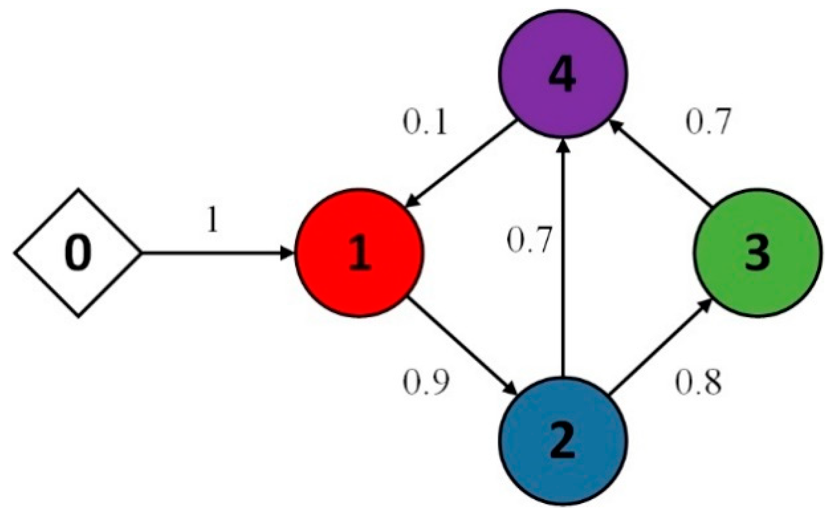
In the domain of uncertain multi-robotic systems, there exists a virtual leader accompanied by N followers. Each follower, identified by $i (\mathrm{ranging} \mathrm{from} 1, 2, \cdots \mathrm{to} N)$, is characterized by the following model

$$\left\{\begin{array}{l}{\dot{x}}_{i,1}=x_{i,2}\\ {\dot{x}}_{i,2}=J_i^{-1}\left(u_i-\left(B_i{x}_{i,2}+G_i{l}_i\sin \left(x_{i,1}\right)\right)\right)\\ y_i=x_{i,1}, \left(i=1,2,\cdots ,N\right)\end{array}\right.$$

(1)

where $x_{i,1}$ and $x_{i,2}$ express angle and angular velocity, respectively, $u_i$ represents the input, and $y_i$ represents the output of the uncertain multi-robotics systems. $J_i$ is the rotational inertia of the robotic arm. $B_i$ represents the frictional viscous coefficient, $G_i=mg$ denotes the gravitational force acting on the robotic arm, and $l_i$ represents the length from the joint axis to the center of mass.

2.2. Graph Theory

In a one-way directed topology, a virtual leader is present alongside N followers. The communication between them is depicted by digraph $\mathrm{G}=\left(\overline{V},E,A,B\right)$. The virtual leader $0$ and followers $i\left(i=1,2,\cdots ,N\right)$ are denoted as $\overline{V}=\left\{0,1,\cdots ,N\right\}$, and $E\in \overline{V}\times \overline{V}$ represents a set of edges. $A={\left[a_{ij}\right]}_{N\times N}$ represents the weighted adjacency matrix of the digraph $\mathrm{G}$, and the edges between follower $j$ and follower $i$ are denoted as ${\overline{V}}_j\times {\overline{V}}_i\in E$. If follower $j$ can obtain data from follower $i$, then $a_{ij}>0$; if not, $a_{ij}=0$. And the $i\text{-}th$ follower degree is represented by $d_i={\displaystyle {\sum }_{j=1,j\ne i}^N{a}_{ij}}$. Its diagonal matrix is $D=diag\left[d_1,d_2,\cdots ,d_N\right]$, and its Laplacian matrix $L$ is $L=D-A\in R^{N\times N}$. Connections from the leader to the followers are symbolized by the weighted adjacency matrix, labeled as $B=diag\left[b_1,b_2,\cdots ,b_N\right]\in R^{N\times N}$. The usage of $b_i>0$ signifies that the $i\text{-}th$ follower can receive messages from the virtual leader, whereas $b_i=0$ indicates the absence of such communication. There exists at least one $b_i$, such that $b_i>0$ ensures $L+B$ is non-singular. At least one path exists from the root node leader $0$ to every follower node, and the digraph can generate a directed tree with the leader $0$ as the root.

Definition 1.

Define the synchronization error of the follower $i$ as follows

$$e_{i,1}={\displaystyle \sum _{j=1}^N{a}_{ij}\left(y_i-y_j\right)}+b_i\left(y_i-y_0\right)$$

(2)

where the reference signal of the leader is denoted by $y_0$.

2.3. Transform Function

Introduce the prescribed performance function as follows

$$E\left(t\right)=\left(E_0-E_{\infty }\right)\exp \left(-t\right)+E_{\infty }$$

(3)

where $E\left(0\right)=E_0$ is the function’s starting value, and $E\left(\infty \right)=E_{\infty }$ is the function’s end value, and they satisfy the condition $E_0>E_{\infty }>0$.

With the aim of enhancing the systems convergence rate, introduce the following speed function

$$s\left(t\right)=\frac{{\left(T-t\right)}^2}{T^2}, t\in \left(0,T\right]$$

(4)

where a prescribed time is denoted by $T$.

Combining Equations (3) and (4), obtain the speed performance function as outlined below

$$E^s\left(t\right)=\left\{\begin{array}{l}\left(E_0-E_{\infty }\right)e^{-t}\frac{{\left(T - t\right)}^2}{T^2}+E_{\infty }, 0<t\le T\\ E_{\infty }, t>T\end{array}\right.$$

(5)

Its inverse satisfies

$$1/E^s\left(t\right)=\left\{\begin{array}{l}\frac{T^2\exp \left(t\right)}{\left(E_0 - E_{\infty }\right){\left(T - t\right)}^2 + E_{\infty }{T}^2\exp \left(t\right)}, 0<t\le T\\ 1/E_{\infty }, t>T\end{array}\right.$$

(6)

According to the above equation, with $\Lambda$ being a positive definite parameter $(\Lambda \le E_0)$, constructed as follows is the transform function

$$k_i\left(t\right)=\left\{\begin{array}{l}\frac{T^2\exp \left(t\right)}{\left(1 - P^{-1}\right){\left(T - t\right)}^2 + P^{-1}{T}^2\exp \left(t\right)}, 0<t\le T\\ P, t>T\end{array}\right.$$

(7)

where the positive definite parameter $P$ satisfies $\Lambda P^{-1}\le E_{\infty }$.

Remark 1.

From the previous derivation and scrutiny, it becomes apparent that the systems’ starting states and systems design parameters have no impact on the prescribed time. The inequality $\Lambda {k_i}^{-1}(t)\le E^s(t)$ always holds, and it holds immense importance for the subsequent deductions and proofs.

2.4. Radial Basis Function Neural Networks

This experiment utilized radial basis function neural networks (RBFNNs) to approximate continuous uncertain nonlinear functions. For function $f\left(\overline{X}\right)$ and a positive definite parameter $\overline{\sigma }$ they satisfy

$$\underset{\overline{X}\in R}{\sup }\left|f\left(\overline{X}\right)-{\Gamma }^T\Theta \left(\overline{X}\right)\right|\le \overline{\sigma }$$

(8)

where $\overline{X}={\left[x_1,x_2,\cdots ,x_p\right]}^T$ represents the input vector, $\Gamma ={\left[{\Gamma }_1,{\Gamma }_2,\cdots ,{\Gamma }_q\right]}^T$ denotes the weight vector, $q>1$ stands for the quantity of NN nodes, and then $\Theta \left(\overline{X}\right)={\left[\Theta {\left(\overline{X}\right)}_1,\Theta {\left(\overline{X}\right)}_2,\cdots ,\Theta {\left(\overline{X}\right)}_q\right]}^T$ represents Gaussian basis functions, which can be expressed as outlined below

$${\Theta }_i\left(\overline{X}\right)=\exp \left(-\frac{{\left({\overline{X}}_i-{\overline{X}}_i^{\ast }\right)}^T\left({\overline{X}}_i-{\overline{X}}_i^{\ast }\right)}{{\upsilon }_i^2}\right)$$

(9)

where the center and width of the Gaussian function are denoted by ${\overline{X}}_i^{\ast }$ and ${\upsilon }_i$, respectively.

Describing ${\Gamma }^{\ast }$ as the optimized weight parameter vector, one can achieve it in the following way

$${\Gamma }^{\ast }=\arg \underset{W\in R}{\min }\left\{\underset{X\in \Omega }{\sup }\left|f\left(\overline{X}\right)-{\Gamma }^T\Theta \left(\overline{X}\right)\right|\right\}$$

(10)

On the compact set $\Omega$, RBFNNs can accurately approximate $f\left(\overline{X}\right)$ with an accuracy of $\sigma \left(\overline{X}\right)$

$$f\left(\overline{X}\right)={\Gamma }^{\ast T}\Theta \left(\overline{X}\right)+\sigma \left(\overline{X}\right)$$

(11)

where $\left|\sigma \left(\overline{X}\right)\right|\le \overline{\sigma }$.

Assumption 1

[41]. $y_0$ expresses the leader reference output signal; it can be denoted by a differentiable, continuous, and bounded function.

3. Control Design and Analysis

3.1. Adaptive NN Prescribed Time Control Design

Coordinate transformations are defined as

$$\left\{\begin{array}{l}{e}_{i,2}=x_{i,2}-{\alpha }_{i,1}, i=1,2,\cdots ,N\\ z_{i,k}=k_i{e}_{i,k}, k=1,2\end{array}\right.$$

(12)

where ${\alpha }_{i,1}$ denotes the virtual control input and $e_{i,1}$, $e_{i,2}$ express error variables.

In accordance with definition (12), the derivative of $z_{i,1}$ is

$$\begin{array}{cc}\hfill {\dot{z}}_{i,1}& =k_i{\dot{e}}_{i,1}+{\dot{k}}_i{e}_{i,1}\hfill \\ & =k_i\left(\left(b_i+d_i\right){\dot{y}}_i-b_i{\dot{y}}_0-{\displaystyle \sum _{j=1}^M{a}_{ij}{\dot{y}}_j}\right)+{\dot{k}}_i{e}_{i,1}\hfill \\ & =k_i\left(\left(b_i+d_i\right)\left(e_{i,2}+{\alpha }_{i,1}\right)-b_i{\dot{y}}_0-{\displaystyle \sum _{j=1}^M{a}_{ij}{\dot{y}}_j}\right)+{\dot{k}}_i{e}_{i,1}\hfill \\ & =k_i\left(\chi e_{i,1}+\left(b_i+d_i\right)\left(e_{i,2}+{\alpha }_{i,1}\right)-b_i{\dot{y}}_0-{\displaystyle \sum _{j=1}^M{a}_{ij}{\dot{y}}_j}\right)\hfill \end{array}$$

(13)

where $\chi =k_i^{-1}{\dot{k}}_i$.

Utilizing the BLFs, select the following BLF $V_{i,1}$

$$V_{i,1}=\frac{1}{2}\log \frac{{\Lambda }_{i,1}^2}{{\Lambda }_{i,1}^2-z_{i,1}^2}+\frac{1}{2{\lambda }_{i,1}}{\tilde{\varphi }}_{i,1}^2$$

(14)

where the positive parameter is ${\lambda }_{i,1}$. The error in adaptive estimation of an unknown constant ${\varphi }_{i,1}=\max \left\{{‖K_{i,1}^{\ast }‖}^2,1\right\}$ is denoted by ${\tilde{\varphi }}_{i,1}={\varphi }_{i,1}-{\widehat{\varphi }}_{i,1}$, then ${\widehat{\varphi }}_{i,1}$ is the estimation value.

Remark 2.

Later, controllers and adaptive laws are established to maintain the boundedness of $V_{i,1}$. And combined with the transform function (7) and BLFs (14), prescribed time control under the given performance is achieved. To further enhance the performance of the systems, similar applications are demonstrated at each step.

Using the derivative of $z_{i,1}$ as a basis, the derivative of $V_{i,1}$ is

$${\dot{V}}_{i,1}=\frac{z_{i,1}{k}_i}{{\Lambda }_{i,1}^2-z_{i,1}^2}\left(\left(b_i+d_i\right)\left(e_{i,2}+{\alpha }_{i,1}\right)+f_{i,1}\left({\overline{X}}_{i,1}\right)\right)-\frac{1}{{\lambda }_{i,1}}{\tilde{\varphi }}_{i,1}{\dot{\widehat{\varphi }}}_{i,1}$$

(15)

where function $f_{i,1}\left({\overline{X}}_{i,1}\right)=\chi e_{i,1}-b_i{\dot{y}}_0-{\displaystyle \sum _{j=1}^N{a}_{ij}{\dot{y}}_j}$, using an NN to deal with it

$$f_{i,1}\left({\overline{X}}_{i,1}\right)={\Gamma }_{i,1}^{\ast T}{\Theta }_{i,1}\left({\overline{X}}_{i,1}\right)+{\sigma }_{i,1}\left({\overline{X}}_{i,1}\right), {\sigma }_{i,1}\left({\overline{X}}_{i,1}\right)\le {\overline{\sigma }}_{i,1}$$

(16)

where ${\overline{X}}_{i,1}={\left[x_{i,1},x_{j,1},x_{j,2},y_0,{\dot{y}}_0\right]}^T$.

The subsequent inequalities are established based on Young’s inequality as follows

$$\frac{\left|z_{i,1}{k}_i\right|\left(b_i+d_i\right)}{{\Lambda }_{i,1}^2-z_{i,1}^2}{e}_{i,2}\le \frac{e_{i,2}^2}{2}+\frac{{\left(b_i+d_i\right)}^2{k}_i^2{z}_{i,1}^2}{2{\left({\Lambda }_{i,1}^2-z_{i,1}^2\right)}^2}$$

(17)

$$\frac{\left|z_{i,1}{k}_i\right|f_{i,i}}{{\Lambda }_{i,1}^2-z_{i,1}^2}\le \frac{k_i^2{z}_{i,1}^2{‖{\Gamma }_{i,1}^{\ast T}‖}^2{‖{\Theta }_{i,1}‖}^2}{2{\hslash }_{i,1}^2{\left({\Lambda }_{i,1}^2-z_{i,1}^2\right)}^2}+\frac{{\hslash }_{i,1}^2}{2}+\frac{k_i^2{z}_{i,1}^2}{2{ƛ}_{i,1}^2{\left({\Lambda }_{i,1}^2-z_{i,1}^2\right)}^2}+\frac{{\overline{\sigma }}_{i,1}^2{ƛ}_{i,1}^2}{2}$$

(18)

where positive designed parameters are denoted as ${\hslash }_{i,1}$ and ${ƛ}_{i,1}$.

Based on the above derivation, one has

$$\begin{array}{cc}\hfill {\dot{V}}_{i,1}\le & \frac{z_{i,1}{k}_i}{{\Lambda }_{i,1}^2 - z_{i,1}^2}\left(b_i+d_i\right){\alpha }_{i,1}+\frac{k_i^2{z}_{i,1}^2{‖{\Gamma }_{i,1}^{\ast T}‖}^2{‖{\Theta }_{i,1}‖}^2}{2{\hslash }_{i,1}^2{\left({\Lambda }_{i,1}^2 - z_{i,1}^2\right)}^2}+\frac{{\hslash }_{i,1}^2}{2}+\frac{k_i^2{z}_{i,1}^2}{2{ƛ}_{i,1}^2{\left({\Lambda }_{i,1}^2 - z_{i,1}^2\right)}^2}\hfill \\ & +\frac{{\overline{\sigma }}_{i,1}^2{ƛ}_{i,1}^2}{2}+\frac{{\left(b_i+d_i\right)}^2{k}_i^2{z}_{i,1}^2}{2{\left({\Lambda }_{i,1}^2 - z_{i,1}^2\right)}^2}+\frac{e_{i,2}^2}{2}-\frac{1}{{\lambda }_{i,1}}{\tilde{\varphi }}_{i,1}{\dot{\widehat{\varphi }}}_{i,1}\hfill \end{array}$$

(19)

Define parameter $Q_{i,1}=\frac{k_{i,1}^2}{2\left({\Lambda }_{i,1}^2-z_{i,1}^2\right)}\left(\frac{1}{{ƛ}_{i,1}^2}+\frac{{‖{\Theta }_{i,1}‖}^2}{{\hslash }_{i,1}^2}+{\left(b_i+d_i\right)}^2\right)$, and the following inequality can be obtained

$${\dot{V}}_{i,1}\le \frac{z_{i,1}{k}_i}{{\Lambda }_{i,1}^2-z_{i,1}^2}\left(\left(b_i+d_i\right){\alpha }_{i,1}+e_{i,1}{Q}_{i,1}{\varphi }_{i,1}\right)+\frac{{\hslash }_{i,1}^2}{2}+\frac{{\overline{\sigma }}_{i,1}^2{ƛ}_{i,1}^2}{2}+\frac{e_{i,2}^2}{2}-\frac{1}{{\lambda }_{i,1}}{\tilde{\varphi }}_{i,1}{\dot{\widehat{\varphi }}}_{i,1}$$

(20)

The virtual controller ${\alpha }_{i,1}$ and adaptive law ${\dot{\widehat{\varphi }}}_{i,1}$ are crafted in the subsequent manner

$${\alpha }_{i,1}=\left(-{\mathcal{l}}_{i,1}{e}_{i,1}-e_{i,1}{\widehat{\varphi }}_{i,1}{Q}_{i,1}\right){\left(b_i+d_i\right)}^{-1}$$

(21)

$${\dot{\widehat{\varphi }}}_{i,1}=-{\xi }_{i,1}{\widehat{\varphi }}_{i,1}+\frac{z_{i,1}^2{\lambda }_{i,1}{Q}_{i,1}}{{\Lambda }_{i,1}^2-z_{i,1}^2}$$

(22)

where ${\mathcal{l}}_{i,1}$ and ${\xi }_{i,1}$ are design parameters that satisfy ${\mathcal{l}}_{i,1}>0$ and ${\xi }_{i,1}>0$.

Integrating controller (21) and adaptive law (22) into Equation (19), it can be obtained that

$${\dot{V}}_{i,1}\le -\frac{{\mathcal{l}}_{i,1}{z}_{i,1}^2}{{\Lambda }_{i,1}^2-z_{i,1}^2}+\frac{{\xi }_{i,1}}{{\lambda }_{i,1}}{\tilde{\varphi }}_{i,1}{\widehat{\varphi }}_{i,1}+\frac{{\hslash }_{i,1}^2}{2}+\frac{{\overline{\tau }}_{i,1}^2{ƛ}_{i,1}^2}{2}+\frac{e_{i,2}^2}{2}$$

(23)

The derivative of $e_{i,2}$ can be obtained as follows

$$\begin{array}{cc}\hfill {\dot{z}}_{i,2}& = {\dot{k}}_i{e}_{i,2}+k_i{\dot{e}}_{i,2}\hfill \\ & ={\dot{k}}_i{e}_{i,2}+k_i\left(J_i^{-1}\left(u_i-G_i{l}_i\sin \left(x_{i,1}\right)-B_i{x}_{i,2}\right)-{\dot{\alpha }}_{i,1}\right)\hfill \\ & =k_i\left(\chi e_{i,2}+J_i^{-1}{u}_i-J_i^{-1}{G}_i{l}_i\sin \left(x_{i,1}\right)-J_i^{-1}{B}_i{x}_{i,2}-{\dot{\alpha }}_{i,1}\right)\hfill \end{array}$$

(24)

Choose the Lyapunov function below

$$V_{i,2}=V_{i,1}+\frac{1}{2}\log \frac{{\Lambda }_{i,2}^2}{{\Lambda }_{i,2}^2-z_{i,2}^2}+\frac{1}{2J_i{\delta }_i}{\tilde{\phi }}_i^2+\frac{1}{2{\lambda }_{i,2}}{\tilde{\varphi }}_{i,2}^2$$

(25)

where ${\lambda }_{i,2}$, ${\delta }_i$ are the design parameters; ${\delta }_i>0$, ${\lambda }_{i,2}>0$, ${\varphi }_{i,2}=\max \left\{{‖K_{i,2}^{\ast }‖}^2,1\right\}$, and ${\phi }_i=J_i$ are the unknowns; ${\widehat{\varphi }}_{i,2}$ and ${\widehat{\phi }}_i$ are the estimation values; and ${\tilde{\varphi }}_{i,2}={\varphi }_{i,2}-{\widehat{\varphi }}_{i,2}$ and ${\tilde{\phi }}_i={\phi }_i-{\widehat{\phi }}_i$ are parameter estimation errors.

Given Equation (13), this leads to the derivative of $V_{i,2}$

$$\begin{array}{cc}\hfill {\dot{V}}_{i,2} =& {\dot{V}}_{i,1}+\frac{z_{i,2}{k}_i}{{\Lambda }_{i,2}^2 - z_{i,2}^2}\left(\chi e_{i,2}+J_i^{-1}{u}_i-J_i^{-1}{B}_i{x}_{i,2}-J_i^{-1}{G}_i{l}_i\sin \left(x_{i,1}\right)-{\dot{\alpha }}_{i,1}\right)\hfill \\ & -\frac{1}{{\lambda }_{i,2}}{\tilde{\varphi }}_{i,2}{\dot{\widehat{\varphi }}}_{i,2}-\frac{1}{J_i{\delta }_i}{\tilde{\phi }}_i{\dot{\widehat{\phi }}}_i\hfill \end{array}$$

(26)

Define the input as $u_i=J_i{\alpha }_{i,2}$, where ${\alpha }_{i,2}$ express the intermediate control input. As ${\phi }_i$ is unknown, the input can be reformulated as

$$\begin{array}{cc}\hfill u_i& ={\widehat{\phi }}_i{\alpha }_{i,2}\hfill \\ & =J_i{\alpha }_{i,2}-{\tilde{\phi }}_i{\alpha }_{i,2}\hfill \end{array}$$

(27)

The following equation is obtained by substituting into Equation (26)

$$\begin{array}{cc}{\dot{V}}_{i,2}=\hfill & {\dot{V}}_{i,m-1}+\frac{z_{i,2}{k}_i}{{\Lambda }_{i,2}^2 - z_{i,2}^2}\left({\alpha }_{i,2}-J_i^{-1}{\tilde{\phi }}_i{\alpha }_{i,2}+f_{i,2}\left({\overline{X}}_{i,2}\right)\right)\hfill \\ & -\frac{1}{{\lambda }_{i,2}}{\tilde{\varphi }}_{i,2}{\dot{\widehat{\varphi }}}_{i,2}-\frac{1}{J_i{\delta }_i}{\tilde{\phi }}_i{\dot{\widehat{\phi }}}_i\hfill \end{array}$$

(28)

where function $f_{i,2}\left({\overline{X}}_{i,2}\right)=\chi e_{i,2}-J_i^{-1}\left(B_i{x}_{i,2}+G_i{l}_i\sin \left(x_{i,1}\right)\right)-{\dot{\alpha }}_{i,1}$, which can be obtained by applying RBFNNs as follows

$$f_{i,2}\left({\overline{X}}_{i,2}\right)={\Gamma }_{i,2}^{\ast T}{\Theta }_{i,2}\left({\overline{X}}_{i,2}\right)+{\sigma }_{i,2}\left({\overline{X}}_{i,2}\right), {\sigma }_{i,2}\left({\overline{X}}_{i,2}\right)\le {\overline{\sigma }}_{i,2}$$

(29)

where ${\overline{X}}_{i,2}={\left[x_{i,1},x_{i,2},x_{j,1},x_{j,2},{\widehat{\varphi }}_{i,1},{\dot{y}}_0\right]}^T$.

The subsequent inequalities can be derived by utilizing Young’s inequality

$$\frac{\left|z_{i,2}{k}_i\right|f_{i,2}}{{\Lambda }_{i,2}^2-z_{i,2}^2}\le \frac{k_i^2{z}_{i,2}^2{‖{\Gamma }_{i,2}^{\ast T}‖}^2{‖{\Theta }_{i,2}‖}^2}{2{\hslash }_{i,2}^2{\left({\Lambda }_{i,2}^2-z_{i,2}^2\right)}^2}+\frac{{\hslash }_{i,2}^2}{2}+\frac{k_i^2{z}_{i,2}^2}{2{ƛ}_{i,2}^2{\left({\Lambda }_{i,2}^2-z_{i,2}^2\right)}^2}+\frac{{\overline{\sigma }}_{i,2}^2{ƛ}_{i,2}^2}{2}$$

(30)

where ${\hslash }_{i,2}$ and ${ƛ}_{i,2}$ are design parameters that satisfy ${\hslash }_{i,2}>0$ and ${ƛ}_{i,2}>0$.

Replacing these inequalities (30) into Equation (28), this yields

$$\begin{array}{cc}\hfill {\dot{V}}_{i,2} \le & {\dot{V}}_{i,1}+\frac{z_{i,2}{k}_i}{{\Lambda }_{i,2}^2 - z_{i,2}^2}{\alpha }_{i,2}+\frac{k_i^2{z}_{i,2}^2{‖{\Gamma }_{i,2}^{\ast T}‖}^2{‖{\Theta }_{i,2}‖}^2}{2{\hslash }_{i,2}^2{\left({\Lambda }_{i,2}^2 - z_{i,2}^2\right)}^2}+\frac{k_i^2{z}_{i,2}^2}{2{ƛ}_{i,2}^2{\left({\Lambda }_{i,2}^2 - z_{i,2}^2\right)}^2}+\frac{{\hslash }_{i,2}^2}{2}\hfill \\ & + \frac{{\overline{\sigma }}_{i,2}^2{ƛ}_{i,2}^2}{2}-\frac{1}{{\lambda }_{i,2}}{\tilde{\varphi }}_{i,2}{\dot{\widehat{\varphi }}}_{i,2}-J_i^{-1}{\tilde{\phi }}_i\left(\frac{z_{i,2}{k}_i{\alpha }_{i,2}}{{\Lambda }_{i,2}^2 - z_{i,2}^2}+{\delta }_i^{-1}{\dot{\widehat{\phi }}}_i\right)\hfill \end{array}$$

(31)

Define $Q_{i,2}=\frac{k_i^2}{2\left({\Lambda }_{i,2}^2-z_{i,2}^2\right)}\left(\frac{{‖{\Theta }_{i,2}‖}^2}{{\hslash }_{i,2}^2}+\frac{1}{{ƛ}_{i,2}^2}+1\right)$, hence

$$\begin{array}{cc}\hfill {\dot{V}}_{i,2} \le & {\dot{V}}_{i,1}+\frac{z_{i,2}{k}_i}{{\Lambda }_{i,2}^2 - z_{i,2}^2}\left({\alpha }_{i,2}+e_{i,2}{Q}_{i,2}{\varphi }_{i,2}\right)+\frac{{\hslash }_{i,2}^2}{2}+\frac{{\overline{\sigma }}_{i,2}^2{ƛ}_{i,2}^2}{2}\hfill \\ & -\frac{1}{{\lambda }_{i,2}}{\tilde{\varphi }}_{i,2}{\dot{\widehat{\varphi }}}_{i,2}-J_i^{-1}{\tilde{\phi }}_i\left(\frac{z_{i,2}{k}_i}{{\Lambda }_{i,2}^2 - z_{i,2}^2}{\alpha }_{i,2}+{\delta }_i^{-1}{\dot{\widehat{\phi }}}_i\right)\hfill \end{array}$$

(32)

To ensure the boundedness of $V_{i,2}$, select the intermediate control input ${\alpha }_{i,2}$, adaptive law ${\dot{\widehat{\varphi }}}_{i,2}$ and ${\dot{\widehat{\phi }}}_i$ as

$${\alpha }_{i,2}=-{\mathcal{l}}_{i,2}{e}_{i,2}-e_{i,2}{\widehat{\varphi }}_{i,2}{Q}_{i,2}-\frac{{\Lambda }_{i,2}^2-z_{i,2}^2}{k_i^2}{e}_{i,2}$$

(33)

$${\dot{\widehat{\varphi }}}_{i,2}=-{\xi }_{i,2}{\widehat{\varphi }}_{i,2}+\frac{z_{i,2}^2{\lambda }_{i,2}{Q}_{i,2}}{{\Lambda }_{i,2}^2-z_{i,2}^2}$$

(34)

$${\dot{\widehat{\phi }}}_i=-{\varsigma }_i{\widehat{\phi }}_i-\frac{z_{i,2}{k}_i{\delta }_i{\alpha }_{i,2}}{{\Lambda }_{i,2}^2-z_{i,2}^2}$$

(35)

where ${\mathcal{l}}_{i,2}$, ${\xi }_{i,2}$, and ${\varsigma }_i$ are design parameters that satisfy ${\mathcal{l}}_{i,2}>0$, ${\xi }_{i,2}>0$ and ${\varsigma }_i>0$.

Substituting controller (33) and adaptive laws (34) and (35) into Equation (32), one has

$$\begin{array}{cc}\hfill {\dot{V}}_{i,2}& \le {\dot{V}}_{i,1}-\frac{{\mathcal{l}}_{i,2}{z}_{i,2}^2}{{\Lambda }_{i,2}^2 - z_{i,2}^2}+\frac{{\delta }_{i,2}}{{\lambda }_{i,2}}{\tilde{\varphi }}_{i,2}{\widehat{\varphi }}_{i,2}+\frac{{\varsigma }_i}{J_i{\delta }_i}{\tilde{\phi }}_i{\widehat{\phi }}_i+\frac{{\hslash }_{i,2}^2}{2}+\frac{{\overline{\sigma }}_{i,2}^2{ƛ}_{i,2}^2}{2}-\frac{e_{i,2}^2}{2}\hfill \\ & =-{\displaystyle \sum _{j=1}^2\frac{{\mathcal{l}}_{i,j}{z}_{i,j}^2}{{\Lambda }_{i,j}^2-z_{i,j}^2}}+{\displaystyle \sum _{j=1}^2\frac{{\delta }_{i,j}}{{\lambda }_{i,j}}{\tilde{\varphi }}_{i,j}{\widehat{\varphi }}_{i,j}}+\frac{{\varsigma }_i}{J_i{\delta }_i}{\tilde{\phi }}_i{\widehat{\phi }}_i+{\displaystyle \sum _{j=1}^2\left(\frac{{\hslash }_{i,j}^2}{2}+\frac{{\overline{\sigma }}_{i,j}^2{ƛ}_{i,j}^2}{2}\right)}\hfill \end{array}$$

(36)

Applying Young’s inequality enables the derivation of the following inequalities

$$\frac{{\delta }_{i,j}}{{\lambda }_{i,j}}{\tilde{\varphi }}_{i,j}{\widehat{\varphi }}_{i,j}\le \frac{{\delta }_{i,j}}{2{\lambda }_{i,j}}{\varphi }_{i,j}^2-\frac{{\delta }_{i,j}}{2{\lambda }_{i,j}}{\tilde{\varphi }}_{i,j}^2$$

(37)

$$\frac{{\varsigma }_i}{J_i{\delta }_i}{\tilde{\phi }}_i{\widehat{\phi }}_i\le \frac{{\varsigma }_i}{2J_i{\delta }_i}{\phi }_i^2-\frac{{\varsigma }_i}{2J_i{\delta }_i}{\tilde{\phi }}_i^2$$

(38)

According to [40], following result holds

$$\log \frac{{\Lambda }_{i,j}^2}{{\Lambda }_{i,j}^2-z_{i,j}^2}\le \frac{z_{i,j}^2}{{\Lambda }_{i,j}^2-z_{i,j}^2}$$

(39)

Substituting Equations (37)–(39) into Equation (36), it can be obtained, as follows, that

$$\begin{array}{cc}\hfill {\dot{V}}_{i,2} \le & -{\displaystyle \sum _{j=1}^2{\mathcal{l}}_{i,j}\log \frac{{\Lambda }_{i,j}^2}{{\Lambda }_{i,j}^2-z_{i,j}^2}}-{\displaystyle \sum _{j=1}^2\frac{{\xi }_{i,j}}{2{\lambda }_{i,j}}{\tilde{\varphi }}_{i,j}^2}-\frac{{\varsigma }_i}{2J_i{\delta }_i}{\tilde{\phi }}_i^2\hfill \\ & +{\displaystyle \sum _{j=1}^2\left(\frac{{\xi }_{i,j}}{2{\lambda }_{i,j}}{\varphi }_{i,j}^2+\frac{{\hslash }_{i,j}^2}{2}+\frac{{\overline{\sigma }}_{i,j}^2{ƛ}_{i,j}^2}{2}\right)}+\frac{{\varsigma }_i}{2J_i{\delta }_i}{\phi }_i^2\hfill \\ \hfill \le & -{\Phi }_{\mathrm{i}}{V}_{i,2}+{\Psi }_i\hfill \end{array}$$

(40)

where ${\Phi }_i={\displaystyle \sum _{j=1}^2\left(\frac{{\xi }_{i,j}}{2{\lambda }_{i,j}}{\varphi }_{i,j}^2+\frac{{\hslash }_{i,j}^2}{2}+\frac{{\overline{\sigma }}_{i,j}^2{ƛ}_{i,j}^2}{2}\right)}+\frac{{\varsigma }_i}{2J_i{\delta }_i}{\phi }_i^2$, ${\Psi }_{\mathrm{i}}=\min \left\{\frac{{\mathcal{l}}_{i,j}}{2},{\xi }_i,{\varsigma }_i\right\}$.

3.2. Multi-Robotics Systems Stability Analysis

For constrained multi-robotic systems with parametric uncertainties, the construction of virtual controllers (Equations (21) and (33)) and adaptive laws (Equations (22), (34) and (35)) enables the realization of the following outcomes:

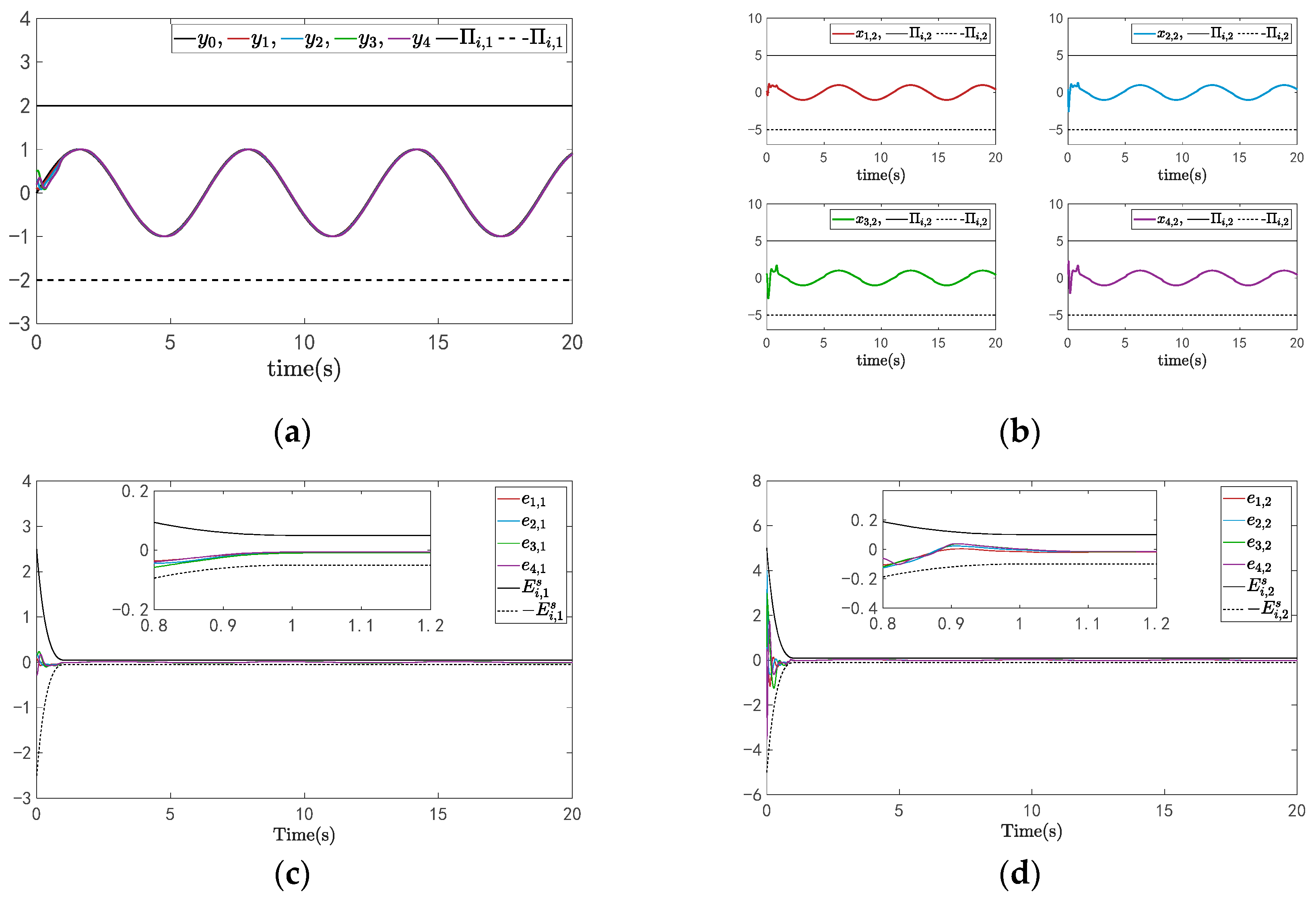
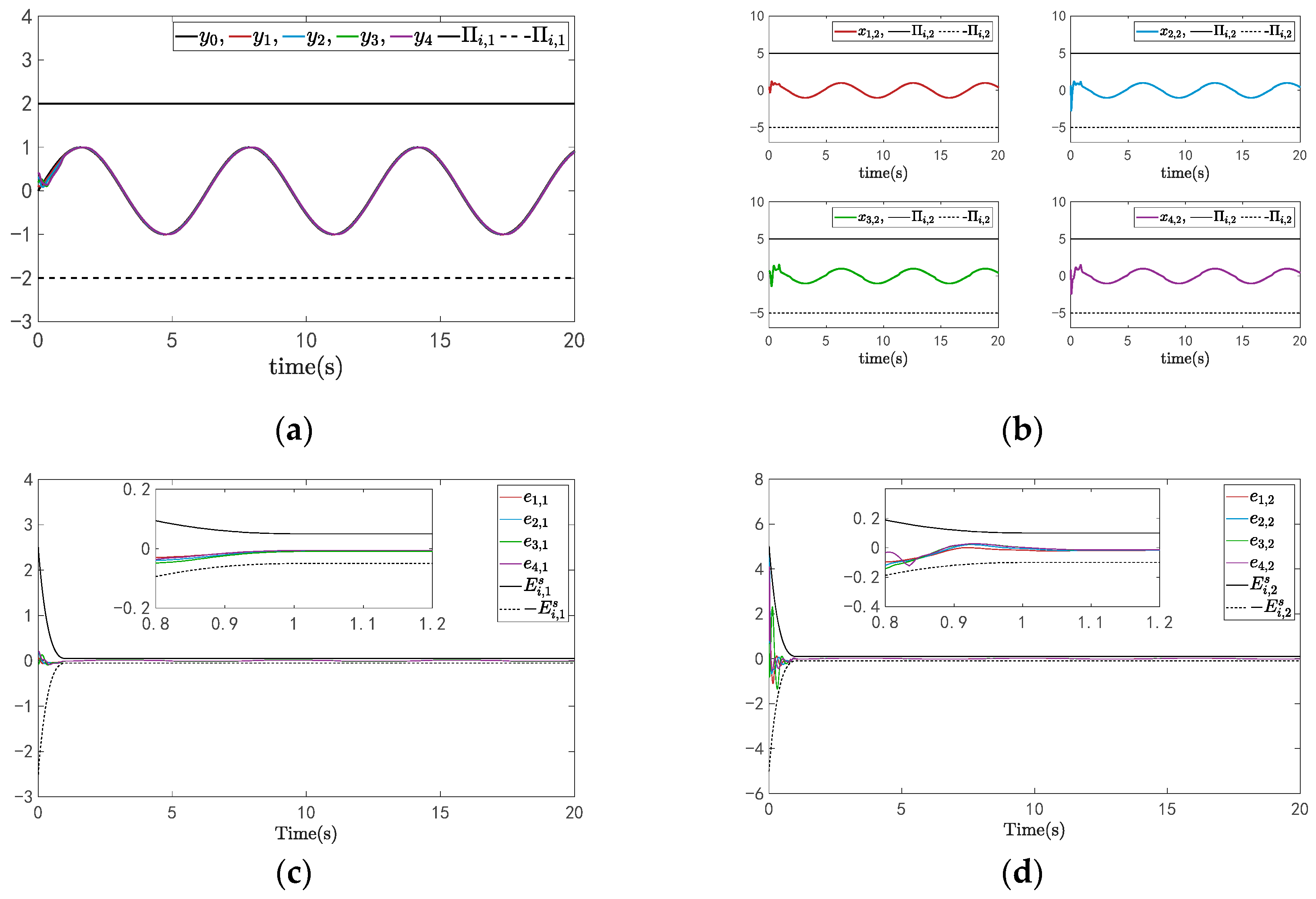
• Signals in multi-robotic systems remain within certain bounds, and systems convergence within a prescribed time $T$, then convergence errors converge in the prescribed regions $\left|e_{i,j}\right|\le P^{-1}{\Lambda }_{i,j}$.
• The systems’ error meets the prescribed performance function $E_{i,j}\left(t\right)$, and the constraints are adhered to by the system states.

Proof of Theorem 1.

Formulated below is the constructed entire Lyapunov function $V$ as follows

$$V={\displaystyle \sum _i^N{V}_{i,2}}$$

(41)

Based on Equation (40), the subsequent equation is derived

$$\dot{V}\le -\Phi V+\Psi$$

(42)

where $\Phi ={\displaystyle \sum _{j=1}^N{\Phi }_i}$, $\Psi =\min \left\{{\Gamma }_{\mathrm{i}},i=1,2,\cdots ,N\right\}$.

By integrating Equation (42), one can derive the resulting expression

$$0\le V\le \frac{\Psi }{\Phi }+e^{-\Psi t}\left(V\left(0\right)-\frac{\Psi }{\Phi }\right)$$

(43)

The boundary of the systems’ errors $z_{i,j}$, ${\tilde{\phi }}_i$, and ${\tilde{\varphi }}_{i,j}$ is evident, and ${\varphi }_{i,j}$ and ${\phi }_i$ are bounded constants, then the boundedness of the estimates ${\widehat{\varphi }}_{i,j}$ and ${\widehat{\phi }}_i$ implies that the virtual controllers ${\alpha }_{i,j}$ are also bounded, according to the definition of virtual controllers. Consequently, both the input and the systems’ signal are bounded.

The function is specified as follows, according to the Lyapunov function

$$\frac{1}{2}\log \frac{{\Lambda }_{i,j}^2}{{\Lambda }_{i,j}^2-z_{i,j}^2}\le e^{-\Psi t}\left(V\left(0\right)-\frac{\Psi }{\Phi }\right)+\frac{\Psi }{\Phi }$$

(44)

Define variable $h=2\left(e^{-\Psi t}\left(V\left(0\right)-\frac{\Psi }{\Phi }\right)+\frac{\Psi }{\Phi }\right)>0$, and the integration of Equation (44) can be acquired through

$$\left|z_{i,j}\right|\le {\Lambda }_{i,j}\sqrt{1-z^{-h}}<{\Lambda }_{i,j}$$

(45)

According to Equation $k_i$(7), it can be obtained, as follows, that

$$\left|e_{i,j}\right| \le \frac{{\Lambda }_{i,j}}{k_i}=\left\{\begin{array}{l}\left(1-P^{-1}\right){\left(\frac{T - t}{T}\right)}^2\exp \left(-t\right){\Lambda }_{i,j}+P^{-1}{\Lambda }_{i,j}, 0\le t<T\\ P^{-1}{\Lambda }_{i,j}, t\ge T\end{array}\right.$$

(46)

According to Equation (46), under the prescribed time $T$, the error attains prescribed areas convergence, satisfying $\left|e_{i,j}\right|\le P^{-1}{\Lambda }_{i,j}$. □

Proof of Theorem 2.

Combined with ${\Lambda }_{i.1}\le E_0$ and $P^{-1}{\Lambda }_{i.1}\le Z_{\infty }$, it can be obtained that $\left(1-P^{-1}\right){\Lambda }_{i.1}\le E_0-E_{\infty }$. In accordance with the function definitions of (5) and (3), the convergence process of error $e_{i,j}\left(t\right)$ satisfies

$$e_{i,j}\left(t\right)\le E_{i,j}^s\left(t\right)\le E_{i,j}\left(t\right)$$

(47)

Hence, the error $e_{i,j}$ satisfies the prescribed performance $E_{i,j}\left(t\right)$.

Remark 3.

Drawing from the earlier derivation, the systems’ convergence time $T$ and the prescribed convergence region $\left|e_{i,j}\right|\le P^{-1}{\Lambda }_{i,j}$ are preset. By enhancing the design parameters ${\mathcal{l}}_{i,j}$, ${\lambda }_{i,j}$, and ${\delta }_i$, and diminishing the design parameters ${\xi }_{i,j}$ and ${\varsigma }_i$, it is evident that $\left|e_{i,j}\right|$ can be reduced. However, regardless of how the aforementioned five design parameters are adjusted, the convergence time and area remain unaffected.

Additionally, based on Equation (46), it is evident that $\left|e_{i,1}\right|\le {\Lambda }_{i,1}/k_i$. Referring to (40), the inequality $\left|y_i-y_d\right|\le \frac{\left|e_{i,1}\right|}{{\pi }_{\min }}$ holds, where ${\pi }_{\min }$ represents the smallest singular value of $L+B$. As $y_d$ satisfies $y_d\le {\overline{y}}_d$, one can derive that $x_{i,1}\le \frac{{\Lambda }_{i,1}}{k_i{\pi }_{\min }}+{\overline{y}}_d$. Define ${\Lambda }_{i,j}=k_i{\pi }_{\min }\left({\Pi }_{i,1}-{\overline{y}}_d\right)$; hence, $x_{i,1}\le {\Pi }_{i,1}$ holds.

Equally, from Equation (46) it is evident that $\left|e_{i,2}\right|\le \frac{{\Lambda }_{i,2}}{k_i}$ holds. Because $e_{i,2}=x_{i,2}-{\alpha }_{i,1}$, therefore $x_{i,2}\le P^{-1}{\Lambda }_{i,2}+{\alpha }_{i,1}$. Define ${\Lambda }_{i,2}=P\left({\overline{\alpha }}_{i,1}+{\Pi }_{i,2}\right)$; hence, $x_{i,1}\le {\Pi }_{i,2}$ holds.

Remark 4.

Although most prescribed time controls emphasize systems convergence time, most of them overlook the issue that rapid convergence progress might lead systems states beyond safe ranges. To tackle this problem, BLFs, prescribed performance function, and speed function are simultaneously applied to achieve quick convergence while ensuring state constraints.

The proof is concluded. □

The proposed adaptive NN control method successfully demonstrated achieving systems convergence with prescribed performance in the presence of parametric uncertainties.

Remark 5.

By constructing BLF and utilizing transform function at every step, the control approach ensures swift convergence of the systems within the prescribed area while avoiding violations of constrained states. Through the incorporation of RBFNNs and the formulation of adaptive laws, systems with uncertain parameters attain the prescribed state within the prescribed time.

4. Simulation Example

The communication topology of the multi-robot system is visualized in Figure 1, including a virtual leader and four followers.

Example

The systems dynamic of follower robotics $i \left(i=1,2,3,4\right)$ can be described as

$$\left\{\begin{array}{l}{\dot{x}}_{i,1}=x_{i,2}, \left(i=1,2,\cdots ,N\right)\\ {\dot{x}}_{i,2}=\frac{1}{J_i}\left(u_i-\left(B_i{x}_{i,2}+G_i{l}_i\sin \left(x_{i,1}\right)\right)\right)\\ y_i=x_{i,1}\end{array}\right.$$

(48)

where $x_{i,1}$ and $x_{i,2}$, respectively, represent the $i\text{-}th$ link angle and angular velocity. Then, $J_i=0.8$ is the inertia moment. $B_i=2$ denotes the viscous friction coefficient of robotics, and $G_i=mg=0.2\times 9.8$ and $l_i=1$ are the mass and length of the $i\text{-}th$ robotics, respectively.

In this example, the system’s prescribed time $T$ was designed as $T=1 s$, and the prescribed performance functions were designed in two steps as $E_{i,1}\left(t\right)=\left(2.5-0.05\right)e^{-t}+0.05$ and $E_{i,2}\left(t\right)=\left(5-0.1\right)e^{-t}+0.1$. Moreover, the parameter of transform function $k_i\left(t\right)$ was designed as ${\Lambda }_{i,1}=2.5$, ${\Lambda }_{i,2}=5$, and $P=50$. And selecting parameters as ${\Pi }_{i,1}=2$ and ${\Pi }_{i,2}=5$, the multi-agent Laplacian matrix $L$ and the degree matrix $D$ were defined as shown below

$$L=\left[\begin{array}{cccc}0.1& 0& 0& -0.1\\ -0.9& 0.9& 0& 0\\ 0& -0.8& 0.8& 0\\ 0& -0.7& -0.7& 1.4\end{array}\right], D=\left[\begin{array}{cccc}1& 0& 0& 0\\ 0& 0& 0& 0\\ 0& 0& 0& 0\\ 0& 0& 0& 0\end{array}\right]$$

(49)

The developed adaptive NN control approach is outlined below

$${\alpha }_{i,1}=\left(-{\mathcal{l}}_{i,1}{e}_{i,1}-e_{i,1}{\widehat{\varphi }}_{i,1}{Q}_{i,1}\right){\left(b_i+d_i\right)}^{-1}$$

(50)

$${\alpha }_{i,2}=-{\mathcal{l}}_{i,2}{e}_{i,2}-e_{i,2}{\widehat{\varphi }}_{i,2}{Q}_{i,2}-\frac{{\Lambda }_{i,2}^2-z_{i,2}^2}{k_i^2}{e}_{i,2}$$

(51)

$${\dot{\widehat{\varphi }}}_{i,1}=-{\xi }_{i,1}{\widehat{\varphi }}_{i,1}+\frac{z_{i,1}^2{\lambda }_{i,1}{Q}_{i,1}}{{\Lambda }_{i,1}^2-z_{i,1}^2}$$

(52)

$${\dot{\widehat{\varphi }}}_{i,2}=-{\xi }_{i,2}{\widehat{\varphi }}_{i,2}+\frac{z_{i,2}^2{\lambda }_{i,2}{Q}_{i,2}}{{\Lambda }_{i,2}^2-z_{i,2}^2}$$

(53)

$${\dot{\widehat{\phi }}}_i=-{\varsigma }_i{\widehat{\phi }}_i-\frac{z_{i,2}{k}_i{\delta }_i{\alpha }_{i,2}}{{\Lambda }_{i,2}^2-z_{i,2}^2}$$

(54)

Below, radial basis functions’ parameters are indicated as

$${\Theta }_i\left(\overline{X}\right)=\exp \left(-\frac{{\left({\overline{X}}_i-{\overline{X}}_i^{\ast }\right)}^T\left({\overline{X}}_i-{\overline{X}}_i^{\ast }\right)}{{\upsilon }_i^2}\right), i=1,2,\cdots ,5$$

(55)

where ${\overline{X}}_{1,1}={\left[x_{1,1},x_{2,1},x_{2,2},y_0,{\dot{y}}_0\right]}^T$, ${\overline{X}}_{2,1}={\left[x_{2,1},x_{3,1},x_{3,2},y_0,{\dot{y}}_0\right]}^T$, ${\overline{X}}_{3,1}={\left[x_{3,1},x_{4,1},x_{4,2},y_0,{\dot{y}}_0\right]}^T$, ${\overline{X}}_{4,1}={\left[x_{4,1},x_{1,1},x_{1,2},y_0,{\dot{y}}_0\right]}^T$, ${\overline{X}}_{1,2}={\left[x_{1,1},x_{1,2},x_{2,1},x_{2,2},{\widehat{\varphi }}_{1,1},y_0,{\dot{y}}_0\right]}^T$, ${\overline{X}}_{2,2}={\left[x_{2,1},x_{2,2},x_{3,1},x_{3,2},{\widehat{\varphi }}_{2,1},y_0,{\dot{y}}_0\right]}^T$, ${\overline{X}}_{3,2}={\left[x_{3,1},x_{3,2},x_{4,1},x_{4,2},{\widehat{\varphi }}_{3,1},y_0,{\dot{y}}_0\right]}^T$, and ${\overline{X}}_{4,2}={\left[x_{4,1},x_{4,2},x_{1,1},x_{1,2},{\widehat{\varphi }}_{4,1},y_0,{\dot{y}}_0\right]}^T$ are the inputs of the RBFNNs. Then, ${\upsilon }_i^2=2$.

Table 1. The initial states and controller parameters of the system.

Case	${\mathit{x}}_{\mathit{i},1}$	${\mathit{x}}_{\mathit{i},2}$	${\mathcal{l}}_{\mathit{i},1}$	${\mathcal{l}}_{\mathit{i},2}$	${\mathit{\lambda }}_{\mathit{i},\mathit{j}}$	${\mathit{\xi }}_{\mathit{i},\mathit{j}}$	${\mathit{\delta }}_{\mathit{i}}$	${\mathit{\varsigma }}_{\mathit{i}}$
I	$\left[0.1,0.3,0.5,0.2\right]$	$\left[0.2,0.4,0.6,0.5\right]$	$\left[30,20,15,22\right]$	$\left[20,10,8,18\right]$	$\left[0.1,0.5\right]$	$\left[5,4\right]$	$1$	$\begin{array}{c}0.1\hfill \end{array}$
II	$\left[0.1,0.3,0.5,0.2\right]$	$\left[0.2,0.4,0.6,0.5\right]$	$\left[25,18,12,20\right]$	$\left[18,13,6,12\right]$	$\left[0.08,0.6\right]$	$\left[3,5\right]$	$1.5$	$0.2$
III	$\left[0.1,0.3,0.2,0.4\right]$	$\left[0.5,0.6,0.7,0.8\right]$	$\left[30,20,15,22\right]$	$\left[20,10,8,18\right]$	$\left[0.1,0.5\right]$	$\left[5,4\right]$	$1$	$\begin{array}{c}0.1\hfill \end{array}$

provides the remaining parameters and initial states.

Figure 2 displays simulation outcomes. The display features both the leader output signal and the follower output signal in Figure 2a. Meanwhile, each follower’s states can be observed in Figure 2b. The followers tracked the leader quickly while adhering to the specified state constraints without any violations, a clarity evident in Figure 2a,b. Figure 2c,d display each follower’s synchronization error and dynamics error. Within the prescribed time $T=1\hspace{0.17em}\mathrm{s}$, the convergence of all errors in the prescribed area became evident, meeting the prescribed performance for convergence progress.

To validate that the starting states and control parameters do not affect the convergence performance and time, while still adhering to the state constraints, two additional simulation experiments were conducted. Each experiment involved different design parameters and varying initial states. Figure 3 and Figure 4 display two simulations’ states and errors. Each follower swiftly converged to the leader without violating state constraints, demonstrating this capability when different parameters or initial states were used. Meeting the prescribed performance within the prescribed time, all errors converged.

Two simulation experiments were carried out (as depicted in Table 1) after adjusting the various design parameters and different initial states listed. Figure 3 and Figure 4 depict the states of the systems and the progress of error convergence. Results from Figure 2, Figure 3 and Figure 4 distinctly indicate that the systems quickly converged within the prescribed performance and prescribed area, even when the parameters were unknown. Furthermore, the state constraints were reliably obeyed. Thus, the confirmation of the effectiveness and feasibility of the advocated control method is evident from these outcomes.

In order to further verify the effectiveness and generality of the proposed method, the authors conducted experiments for different initial states and different control parameters, and the specific initial states and controller parameters are shown in Table 1.

Figure 3 and Figure 4 depict the states of the systems and the progress of error convergence, and similar control effects were obtained. Results from Figure 2, Figure 3 and Figure 4 distinctly indicate that the systems quickly converged within the prescribed performance and prescribed area, even when the parameters were unknown. Furthermore, the state constraints were reliably obeyed. Figure 3 and Figure 4 display two simulations’ states and errors. Each follower swiftly converged to the leader without violating state constraints, demonstrating this capability when different parameters or initial states were used. Within the prescribed time, all errors converged under the prescribed performance. Thus, the confirmation of the effectiveness and feasibility of the advocated control method is evident from these outcomes.

5. Conclusions

Under the influence of parametric uncertainties, this study explored achieving prescribed performance in constrained multi-robotic systems. Using an adaptive NN control approach, the challenge was tackled. Adaptive laws and RBFNNs, employed to manage the impact of unknown parameters, effectively countered their effects. Regardless of any existing parametric uncertainties, the proposed control approach ensured that all followers achieved the predefined precision within the prescribed time. The viability demonstrated here pertains to the proposed control approach through some simulations. In future, we will focus on refining our control strategy to address a broader range of uncertainties and exploring its applicability to various robotic applications. This includes examining additional uncertainties, such as environmental disturbances, sensor noise, and communication delays, as well as adapting our strategy for use in autonomous vehicles, industrial automation, and unmanned aerial vehicles (UAVs).

References

1. He, S.; Xu, Y.; Wu, Y.; Li, Y.; Zhong, W. Adaptive consensus tracking of multi-robotic systems via using integral sliding mode control. Neurocomputing 2021, 455, 154–162. [Google Scholar] [CrossRef]
2. Liu, D.; Liu, Z.; Chen, C.P.; Zhang, Y. Prescribed-time containment control with prescribed performance for uncertain nonlinear multi-agent systems. J. Frankl. Inst. 2021, 358, 1782–1811. [Google Scholar] [CrossRef]
3. Dai, S.; Wu, Z.; Li, S.; Wang, J.; Tan, M.; Yu, J. Model-Based Event-Triggered Dynamic Pursuing and Surrounding Control for a Multi-Robotic Fish System. IEEE Robot. Autom. Lett. 2023, 8, 3788–3795. [Google Scholar] [CrossRef]
4. Behera, L.; Rybak, L.; Malyshev, D.; Gaponenko, E. Determination of workspaces and intersections of robot links in a multi-robotic system for trajectory planning. Appl. Sci. 2021, 11, 4961. [Google Scholar] [CrossRef]
5. Jia, H.; Zhao, Y.; Zhai, Y.; Ding, B.; Wang, H.; Wu, Q. Crmrl: Collaborative relationship meta reinforcement learning for effectively adapting to type changes in multi-robotic system. IEEE Robot. Autom. Lett. 2022, 7, 11362–11369. [Google Scholar] [CrossRef]
6. Fang, Y.; Ming, H.; Li, M.; Liu, Q.; Pham, D.T. Multi-objective evolutionary simulated annealing optimisation for mixed-model multi-robotic disassembly line balancing with interval processing time. Int. J. Prod. Res. 2020, 58, 846–862. [Google Scholar] [CrossRef]
7. Sanila, P.; Pradeep, A.; Jacob, J.; Ramchand, R. Leader–follower target interception control of multi-robotic vehicles with holonomic dynamics based on unscented Kalman filter. Nonlinear Dyn. 2023, 111, 11171–11190. [Google Scholar] [CrossRef]
8. Klančar, G.; Seder, M. Coordinated Multi-Robotic Vehicles Navigation and Control in Shop Floor Automation. Sensors 2022, 22, 1455. [Google Scholar] [CrossRef]
9. Wang, Z.; Zhou, B.; Trentesaux, D.; Bekrar, A. Approximate optimal method for cyclic solutions in multi-robotic cell with processing time window. Robot. Auton. Syst. 2017, 98, 307–316. [Google Scholar] [CrossRef]
10. Din, A.; Ismail, M.Y.; Shah, B.; Babar, M.; Ali, F.; Baig, S.U. A deep reinforcement learning-based multi-agent area coverage control for smart agriculture. Comput. Electr. Eng. 2022, 101, 108089. [Google Scholar] [CrossRef]
11. Mishra, R.; Bajpai, M.K. Hybrid multiagent based adaptive genetic algorithm for limited view tomography using oppositional learning. Biomed. Signal Process. Control 2022, 75, 103610. [Google Scholar] [CrossRef]
12. Nilsson, A.; Danielsson, F.; Svensson, B. Customization and flexible manufacturing capacity using a graphical method applied on a configurable multi-agent system. Robot. Comput.-Integr. Manuf. 2023, 79, 102450. [Google Scholar] [CrossRef]
13. Leng, J.; Sha, W.; Lin, Z.; Jing, J.; Liu, Q.; Chen, X. Blockchained smart contract pyramid-driven multi-agent autonomous process control for resilient individualised manufacturing towards Industry 5.0. Int. J. Prod. Res. 2023, 61, 4302–4321. [Google Scholar] [CrossRef]
14. Li, D.; Ge, S.S.; Lee, T.H. Fixed-time-synchronized consensus control of multiagent systems. IEEE Trans. Control Netw. Syst. 2020, 8, 89–98. [Google Scholar] [CrossRef]
15. Wang, X.; Su, H. Consensus of multiagent with interaction distortions via echo control. Inf. Sci. 2022, 614, 518–533. [Google Scholar] [CrossRef]
16. Wang, G.; Wang, C.; Cai, X. Consensus control of output-constrained multiagent systems with unknown control directions under a directed graph. Int. J. Robust Nonlinear Control 2020, 30, 1802–1818. [Google Scholar] [CrossRef]
17. Wang, W.; Li, Y. Distributed fuzzy optimal consensus control of state-constrained nonlinear strict-feedback systems. IEEE Trans. Cybern. 2022, 53, 2914–2929. [Google Scholar] [CrossRef] [PubMed]
18. Wang, J.L.; Han, X.; Huang, T. PD and PI Control for the Lag Consensus of Nonlinear Multiagent Systems with and Without External Disturbances. IEEE Trans. Cybern. 2023, 54, 3716–3726. [Google Scholar] [CrossRef] [PubMed]
19. Wang, X.; Wang, G.; Li, S.; Lu, K. Composite sliding-mode consensus algorithms for higher-order multi-agent systems subject to disturbances. IET Control Theory Appl. 2020, 14, 291–303. [Google Scholar] [CrossRef]
20. Xu, C.; Wu, B.; Zhang, Y. Distributed prescribed-time attitude cooperative control for multiple spacecraft. Aerosp. Sci. Technol. 2021, 113, 106699. [Google Scholar] [CrossRef]
21. Ye, H.; Song, Y. Prescribed-time control for linear systems in canonical form via nonlinear feedback. IEEE Trans. Syst. Man Cybern. Syst. 2022, 53, 1126–1135. [Google Scholar] [CrossRef]
22. Ren, Y.; Zhou, W.; Li, Z.; Liu, L.; Sun, Y. Prescribed-time cluster lag consensus control for second-order non-linear leader-following multiagent systems. ISA Trans. 2021, 109, 49–60. [Google Scholar] [CrossRef] [PubMed]
23. Ning, B.; Han, Q.-L.; Zuo, Z.; Ding, L.; Lu, Q.; Ge, X. Fixed-time and prescribed-time consensus control of multiagent systems and its applications: A survey of recent trends and methodologies. IEEE Trans. Ind. Inform. 2022, 19, 1121–1135. [Google Scholar] [CrossRef]
24. Wang, Y.; Song, Y.; Hill, D.J.; Krstic, M. Prescribed-time consensus and containment control of networked multiagent systems. IEEE Trans. Cybern. 2018, 49, 1138–1147. [Google Scholar] [CrossRef] [PubMed]
25. Chen, X.; Yu, H.; Hao, F. Prescribed-time event-triggered bipartite consensus of multiagent systems. IEEE Trans. Cybern. 2020, 52, 2589–2598. [Google Scholar] [CrossRef] [PubMed]
26. Dai, L.; Chen, X.; Guo, L.; Zhang, J.; Chen, J. Prescribed-time Group Consensus for Multiagent System Based on a Distributed Observer Approach. Int. J. Control Autom. Syst. 2022, 20, 3129–3137. [Google Scholar] [CrossRef]
27. Zhu, P.; Hong, X.; Yang, D. Disturbance observer-based controller design for uncertain nonlinear parameter-varying systems. ISA Trans. 2022, 130, 265–276. [Google Scholar] [CrossRef] [PubMed]
28. Yan, Y.; Wang, X.; Li, Y.; Zeng, L.; Li, Y.; Wang, L. Importance measure analysis of design variables and uncertain parameters in multidisciplinary systems. Appl. Math. Model. 2022, 107, 296–315. [Google Scholar] [CrossRef]
29. Zhao, J.; Lin, C.M. Wavelet-TSK-type fuzzy cerebellar model neural network for uncertain nonlinear systems. IEEE Trans. Fuzzy Syst. 2018, 27, 549–558. [Google Scholar] [CrossRef]
30. Zhang, Z.; Wang, Q.; Sang, Y.; Ge, S.S. Globally Adaptive Neural Network Output-Feedback Control for Uncertain Nonlinear Systems. IEEE Trans. Neural Netw. Learn. Syst. 2022, 34, 9078–9087. [Google Scholar] [CrossRef]
31. Li, Y.; Min, X.; Tong, S. Adaptive fuzzy inverse optimal control for uncertain strict-feedback nonlinear systems. IEEE Trans. Fuzzy Syst. 2019, 28, 2363–2374. [Google Scholar] [CrossRef]
32. Wang, Q.; Zhang, Z.; Xie, X.J. Globally adaptive neural network tracking for uncertain output-feedback systems. IEEE Trans. Neural Netw. Learn. Syst. 2021, 34, 814–823. [Google Scholar] [CrossRef] [PubMed]
33. Chen, Z.; Niu, B.; Zhang, L.; Zhao, J.; Ahmad, A.M.; Alassafi, M.O. Command filtering-based adaptive neural network control for uncertain switched nonlinear systems using event-triggered communication. Int. J. Robust Nonlinear Control 2022, 32, 6507–6522. [Google Scholar] [CrossRef]
34. Ding, B.; Pan, Y.; Lu, Q. Neural adaptive optimal control for nonlinear multiagent systems with full-state constraints and immeasurable states. Neurocomputing 2023, 544, 126259. [Google Scholar] [CrossRef]
35. Xu, Z.; Deng, W.; Shen, H.; Yao, J. Extended-state-observer-based adaptive prescribed performance control for hydraulic systems with full-state constraints. IEEE/ASME Trans. Mechatron. 2022, 27, 5615–5625. [Google Scholar] [CrossRef]
36. Duan, J.; Liu, Z.; Li, S.E.; Sun, Q.; Jia, Z.; Cheng, B. Adaptive dynamic programming for nonaffine nonlinear optimal control problem with state constraints. Neurocomputing 2022, 484, 128–141. [Google Scholar] [CrossRef]
37. Ji, Q.; Chen, G.; He, Q. Neural network-based distributed finite-time tracking control of uncertain multi-agent systems with full state constraints. IEEE Access 2020, 8, 174365–174374. [Google Scholar] [CrossRef]
38. Xu, Z.; Qi, G.; Liu, Q.; Yao, J. ESO-based adaptive full state constraint control of uncertain systems and its application to hydraulic servo systems. Mech. Syst. Signal Process. 2022, 167, 108560. [Google Scholar] [CrossRef]
39. Liu, R.; Liu, M.; Shi, Y.; Qu, J. Adaptive Fixed-Time Fuzzy Control for Uncertain Nonlinear Systems with Asymmetric Time-Varying Full-State Constraints. Int. J. Fuzzy Syst. 2023, 25, 1597–1611. [Google Scholar] [CrossRef]
40. Wang, J.; Yan, Y.; Liu, Z.; Chen, C.P.; Zhang, C.; Chen, K. Finite-time consensus control for multi-agent systems with full-state constraints and actuator failures. Neural Netw. 2023, 157, 350–363. [Google Scholar] [CrossRef]
41. Li, Y.; Li, K.; Tong, S. An observer-based fuzzy adaptive consensus control method for nonlinear multiagent systems. IEEE Trans. Fuzzy Syst. 2022, 30, 4667–4678. [Google Scholar] [CrossRef]
Figure 1. Communication topology.
Mathematics 12 01880 g001
Figure 2. Simulations results for Example case I. (a) Outputs of all followers; (b) states of all followers; (c) synchronization errors of all followers; and (d) dynamics errors of all followers.
Mathematics 12 01880 g002
Figure 3. Simulations results for Example case II. (a) Outputs of all followers; (b) states of all followers; (c) synchronization errors of all followers; and (d) dynamics errors of all followers.
Mathematics 12 01880 g003
Figure 4. Simulations results for Example case III. (a) Outputs of all followers; (b) states of all followers; (c) synchronization errors of all followers; and (d) dynamics errors of all followers.
Mathematics 12 01880 g004