An Underwater Passive Electric Field Positioning Method Based on Scalar Potential

Abstract

In order to fulfill the practical application demands of precisely localizing underwater vehicles using passive electric field localization technology, we propose a scalar-potential-based method for the passive electric field localization of underwater vehicles. This method is grounded on an intelligent differential evolution algorithm and is particularly suited for use in three-layer and stratified oceanic environments. Firstly, based on the potential distribution law of constant current elements in a three-layer parallel stratified ocean environment, the mathematical positioning model is established using the mirror method. Secondly, the differential evolution (DE) algorithm is enhanced with a parameter-adaptive strategy and a boundary mutation processing mechanism to optimize the key objective function in the positioning problem. Additionally, the simulation experiments of the current element in the layered model prove the effectiveness of the proposed positioning method and show that it has no special requirements for the sensor measurement array, but the large range and moderate number of sensors are beneficial to improve the positioning effect. Finally, the laboratory experiments on the positioning method proposed in this paper, involving underwater simulated current elements and underwater vehicle tracks, were carried out successfully. The results indicate that the positioning method proposed in this paper can achieve the performance requirements of independent initial value, strong anti-noise capabilities, rapid positioning speed, easy implementation, and suitability in shallow sea environments. These findings suggest a promising practical application potential for the proposed method.

1. Introduction

The detection of underwater vehicles has been the focus of attention in the field of underwater target detection globally for some time. Especially with the continuous development of noise reduction [1] and degaussing [2] technologies, positioning technology that relies solely on target acoustic signals and magnetic signals is becoming increasingly obsolete. The current data indicate that the noise spectrum levels of silent underwater vehicles developed by countries such as the United Kingdom, the United States, and Russia are even lower than the ocean background noise [1,3], posing a significant challenge for the detection of underwater vehicles using sonar. Therefore, the pursuit of novel underwater vehicle signal radiation sources and the development of corresponding underwater vehicle target detection technologies are not only crucial for practical applications such as the search, rescue, and recovery of lost underwater vehicles; positioning, display, and navigation of underwater robots; maritime traffic safety warnings; and detection of underwater military targets, but also hold tremendous potential research value in areas such as the localization and identification of underwater obstacles with radiation sources, leak repair and detection for submarine pipelines, and other underwater operations or ocean exploration. In this context, leveraging the underwater electric fields of underwater vehicles for the independent or auxiliary detection and localization of targets presents significant advantages.

Prior research has demonstrated that underwater vehicles’ static electric field originates from corrosion and anti-corrosion currents, possessing a significant amount of energy that poses challenges in achieving complete control or elimination. The scalar potential generated several kilometers away can still attain magnitudes reaching tens of nanovolts, thereby providing the potential for utilizing remote electric fields to achieve the detection of underwater vehicles [4]. Given that the far-field source of the underwater vehicle’s electrostatic field can be considered to be a constant current element [5], the task of locating an underwater vehicle’s electric field over long distances in shallow seas can be reduced to the problem of passively locating a constant current element within a stratified marine environment.

Numerous studies have been conducted domestically and internationally on passive electric field positioning models, devices, and algorithms for constant current elements in stratified marine environments. However, there remain certain limitations in this field. Regarding the selection of location field models, the majority of studies opt for infinite sea areas (non-stratified fields) or semi-infinite sea areas (two-layer stratified fields) as their positioning models [6,7]. The shallow sea (three-layer stratified field) model is infrequently chosen, primarily due to the significant increase in complexity associated with inversion algorithms as the number of media interfaces rises [8,9,10]. Nevertheless, if the application scenario does not align with the assumptions of infinite or semi-infinite fields, the mismatch in positioning models can inevitably lead to a reduction in positioning accuracy. In terms of selecting physical positioning quantities, the current options for electric field positioning primarily encompass three-component electric field intensity or potential measurement values relative to a reference point [11,12]. Given that scalar potential functions can effectively describe static field distributions, potential measurements offer a convenient and computationally simplified approach to data processing, thereby favoring practical applications [13]. Regarding the choice of location algorithms, two primary approaches emerge: field source parameter fitting based on numerical calculations [14,15,16,17,18], and field source parameter inversion leveraging intelligent optimization algorithms [12,19,20]. The former typically requires fewer measurement points, less computational intensity, and faster operation speeds; however, it also exhibits a strong dependence on initial values and limited noise resilience and is primarily suitable for near-field applications. In contrast, the latter incorporates intelligent algorithms, such as improved particle swarm optimization, simulated annealing, fuzzy fusion estimation, neural networks, and Kalman filters, which can effectively address issues related to initial-value dependency. Nevertheless, these approaches still face challenges, such as limited positioning ranges, susceptibility to local optimal solutions, and low positioning space dimensions. Furthermore, concerning the arrangement of detection sensors, there is no singular optimal configuration for the deployment of electric field detection sensors. This includes configurations such as positioning two three-component field strength measurement points [14,18,21] or designing arrays distributed in rectangular, circular, cross, and stereo patterns [7,12,22,23]. Typically, the optimal layout needs to be tailored based on specific application requirements and the inversion algorithm employed, necessitating a customized optimization process.

In the practical application of underwater vehicle passive electric field positioning technology, it is often imperative to possess a substantial positioning range extending several kilometers, robust anti-noise capabilities, a relatively flexible sensor arrangement, and excellent real-time performance. Additionally, it is essential to operate in shallow sea environments, particularly in stratified media consisting of air, seawater, and seabed. A feasible positioning approach involves randomly deploying multi-electrode arrays within a designated area, where the relative positions of the electrodes are known and can be easily identified. Subsequently, intelligent optimization algorithms can be utilized to calculate target parameters, specifically field source parameters, through the potential signals measured by each electrode. This paper utilizes an intelligent differential evolution algorithm to investigate a passive electric field localization method based on scalar potential for detecting underwater vehicles. This approach is tailored for three-layer stratified marine environments. Through meticulous simulation and laboratory testing, the results demonstrate that the established positioning method can effectively locate the target, independent of the initial values; it boasts a vast positioning range, robust anti-noise capabilities, and a reduced likelihood of falling into local optimal solutions, exhibiting strong practical application prospects.

2. Positioning Method

2.1. Three-Layer Positioning Model

Considering the shallow sea model, as shown in Figure 1, the space V, permittivity ε, and conductivity σ corresponding to the air, seawater, and seabed are represented by the subscripts 0, 1, and 2, respectively, and the seawater depth is D. Taking the interface between air and seawater as the xoy plane and vertically downward as the positive direction of the z-axis, a rectangular coordinate system is established. Assuming that the equivalent field source of the underwater robot’s electrostatic field is located at M₀, with a position vector r₀ = (x₀, y₀, z₀) and an equivalent field source intensity of p (p_x, p_y, p_z), the directed line segments r-r_0± represent the directions from the current source or sink points (with position vectors r_0±) to the field point. Num measuring points are set in the water, the position coordinates of the measuring points are known, and the position vector of the i-th measuring point M_i is represented by r_i = (x_i, y_i, z_i), i =1, 2, …, Num. In addition, Idl represents a constant current element, which is an electrical analog body; I is the current carried by the target; dl represents the distance between the source and sink of the current; R_i represents the distance between the current element and each measurement point M_i; and Σ₁ and Σ₂ represent the two boundary interfaces shown in the Figure 1.

According to the principles of electromagnetic field theory, the field source p induces a steady-state current field in conductive media such as seawater and the seabed, while an electrostatic field is established in insulating media. Consequently, at the interface between regions V₀ and V₁, the scalar potential is continuous, and the normal component of the electric displacement vector is zero, satisfying the relevant boundary conditions. Similarly, at the interface between V₁ and V₂, both the scalar potential and the normal component of the current density vector remain continuous, fulfilling the corresponding boundary conditions. Based on these conditions, the scalar potential at the field point M_i satisfies the following well-posed problem:

$$\left\{\begin{array}{l}{\nabla }^2{\phi }_{{\sigma }_1}\left(\mathit{r}\right)=-\frac{I\left[\delta \left(\mathit{r}-{\mathit{r}}_{0+}\right)-\delta \left(\mathit{r}-{\mathit{r}}_{0-}\right)\right]}{{\sigma }_1},\left({\mathrm{M}}_i\in {\mathrm{V}}_1\right)\\ {\nabla }^2{\phi }_{\epsilon }\left(\mathit{r}\right)=0,\left({\mathrm{M}}_i\in {\mathrm{V}}_0\right)\\ {\phi }_{{\sigma }_1}\left(\mathit{r}\right){|}_{{\Sigma }_1}={\phi }_{\epsilon }\left(\mathit{r}\right){|}_{{\Sigma }_1}\\ {\sigma }_1\mathit{n}·\nabla {\phi }_{{\sigma }_1}\left(\mathit{r}\right){|}_{{\Sigma }_1}=0\\ {\nabla }^2{\phi }_{{\sigma }_2}\left(\mathit{r}\right)=0,\left({\mathrm{M}}_i\in {\mathrm{V}}_2\right)\\ {\phi }_{{\sigma }_1}\left(\mathit{r}\right){|}_{{\Sigma }_2}={\phi }_{{\sigma }_2}\left(\mathit{r}\right){|}_{{\Sigma }_2}\\ {\sigma }_1\mathit{n}·\nabla {\phi }_{{\sigma }_1}\left(\mathit{r}\right){|}_{{\Sigma }_2}={\sigma }_2\mathit{n}·\nabla {\phi }_{{\sigma }_2}\left(\mathit{r}\right){|}_{{\Sigma }_2}\end{array}\right.$$

(1)

Given that underwater vehicles are typically deployed for seabed operations or require reduced water depth to achieve certain stealth navigation requirements, the impact of the seabed on the field distribution cannot be overlooked in the study of the electric field target characteristics of underwater vehicles. Additionally, due to technological constraints, it is currently difficult for underwater vehicles to operate at great depths, rendering the influence of air on the field distribution equally significant. Therefore, choosing the shallow sea (seabed–ocean–air) environment as the model for analysis is highly relevant to practical applications and possesses a certain research value. Given the presence of two medium interfaces in the three-layer ocean model, it is necessary to consider the influence of each interface of different media on the studied field domain, which complicates the solution of electromagnetic field distribution. Typically, approximate calculations or numerical solutions are employed to handle mathematical expressions with complex Fourier–Bessel integrals [24,25], which are not conducive to subsequent modeling, simulation, or mathematical optimization operations and are only suitable for solving forward problems where the electric field distribution is predicted based on known electric field parameters, thereby exhibiting significant limitations. Consequently, based on the uniqueness theorem, the image method is selected to analyze and solve the impact of each interface separately, significantly reducing the computational complexity. This approach also enables the inversion problem of deducing field source parameters by measuring electric field distribution data without knowing any parameters, making it highly suitable for localization problems. The chosen field point M_i is consistently located in the seawater region V₁. Firstly, for the conductive media of seawater and seabed, the current element mirror p′ (with position vector r₀′) and p are symmetric at the interface, and the electric field generated by p at point M_i is equivalent to the combined electric field generated by p′ and p at point M_i when the entire space is filled with medium σ₁. To solve the simultaneous equations, a field point M_i′ in V₂ is assumed, and p has the same mirror position. The combined field source intensity of the two is denoted as p″. At this point, the electric field generated by p at M_i′ is equivalent to the electric field generated by p″ at M_i′ when the entire space is filled with medium σ₂, as shown in the following equation:

$$\left\{\begin{array}{l}{\phi }_{{\sigma }_1}\left(\mathit{r}\right)=\frac{\mathit{p}·\mathit{R}}{4\pi {\sigma }_1{R}^3}+\frac{{\mathit{p}}^{\prime }·{\mathit{R}}^{\prime }}{4\pi {\sigma }_{1}R{\prime }^3},\left({\mathrm{M}}_i\in {\mathrm{V}}_1\right)\\ {\phi }_{{\sigma }_2}\left(\mathit{r}\right)=\frac{{\mathit{p}}^{″}·\mathit{R}}{4\pi {\sigma }_2{R}^3},\left({\mathrm{M}}_i\in {\mathrm{V}}_2\right)\end{array}\right.,$$

(2)

where $\mathit{R}=\mathit{r}-{\mathit{r}}_0$ and $\mathit{R}\prime =\mathit{r}-\mathit{r}{\prime }_0$ represent the radial vectors of the field point and the field source or the field source mirror, respectively. The computation of R and R′ becomes feasible when the positions of the field source and field point are known. In the above formula, ${\phi }_{{\sigma }_1}\left(\mathit{r}\right)$ and ${\phi }_{{\sigma }_2}\left(\mathit{r}\right)$ represent the potential of the field point in medium σ₁ and medium σ₂, respectively. Furthermore, the derivation of Expression (2) from (1), based on the boundary conditions, can be achieved with the aid of the Cartesian coordinate system established previously, which facilitates the determination of p′ and p″.

Let $\mathit{Q}=diag\left(1,1,-1\right)$, where the points on the boundary surface satisfy the following relationship:

$$\left\{\begin{array}{l}\mathit{R}\prime {|}_{\Sigma }=\mathit{R}\mathit{Q}{|}_{\Sigma }\\ \\ R\prime {|}_{\Sigma }=R{|}_{\Sigma }\end{array}\right.,$$

(3)

which can be substituted into the boundary conditions of Equation (1) along with Equation (2), and the Σ after the variable indicates that the condition is satisfied on this surface, leading to the derivation of the following system of equations:

$$\left\{\begin{array}{l}\frac{\mathit{p}·\mathit{R}{|}_{\Sigma }+{\mathit{p}}^{\prime }·\left(\mathit{R}\mathit{Q}{|}_{\Sigma }\right)}{{\sigma }_1}=\frac{{\mathit{p}}^{″}·\mathit{R}{|}_{\Sigma }}{{\sigma }_2}\\ \frac{-\mathit{n}·\left(\mathit{p}+{\mathit{p}}^{\prime }\right)}{R{{|}_{\Sigma }}^3}+3\frac{\mathit{n}·[(\mathit{p}·\mathit{R}{|}_{\Sigma })\mathit{R}{|}_{\Sigma }]+\mathit{n}·[({\mathit{p}}^{\prime }·\left(\mathit{R}\mathit{Q}{|}_{\Sigma }\right))\left(\mathit{R}\mathit{Q}{|}_{\Sigma }\right)]}{R{{|}_{\Sigma }}^5}=\frac{-\mathit{n}·{\mathit{p}}^{″}}{R{{|}_{\Sigma }}^3}+3\frac{\mathit{n}·[({\mathit{p}}^{″}·\mathit{R}{|}_{\Sigma })\mathit{R}{|}_{\Sigma }]}{R{{|}_{\Sigma }}^5}\end{array}\right.,$$

(4)

where p and R are arbitrary and n represents the normal vector; it is possible to simplify the system of equations into the following form:

$$\left\{\begin{array}{l}\frac{{\sigma }_2}{{\sigma }_1}\left(\mathit{p}·\mathit{R}{|}_{\Sigma }+{\mathit{p}}^{\prime }·\mathit{R}\mathit{Q}{|}_{\Sigma }\right)={\mathit{p}}^{″}·\mathit{R}{|}_{\Sigma }\\ \mathit{p}·\mathit{R}{|}_{\Sigma }-{\mathit{p}}^{\prime }·\mathit{R}\mathit{Q}{|}_{\Sigma }={\mathit{p}}^{″}·\mathit{R}{|}_{\Sigma }\end{array}\right.$$

(5)

Since p and p′ are three-dimensional vectors under the same basis, the relationship between p and p′ can be expressed by a 3 × 3 transformation matrix X, i.e., p = X p′. Substituting this into Equation (5) yields the following relationship:

$$\frac{{\sigma }_2}{{\sigma }_1}\left(\mathit{p}·\mathit{R}{|}_{\Sigma }+\mathit{p}\mathit{X}·\mathit{R}\mathit{Q}{|}_{\Sigma }\right)=\mathit{p}·\mathit{R}{|}_{\Sigma }-\mathit{p}\mathit{X}·\mathit{R}\mathit{Q}{|}_{\Sigma },$$

(6)

which can be transformed through the relation $\mathit{p}\mathit{X}·\mathit{R}\mathit{Q}{|}_{\Sigma }=\mathit{p}\mathit{X}\mathit{Q}·\mathit{R}{|}_{\Sigma }$, resulting in the following expression:

$$\left(\frac{{\sigma }_2}{{\sigma }_1}+1\right)\mathit{p}\mathit{X}\mathit{Q}·\mathit{R}{|}_{\Sigma }=\left(1-\frac{{\sigma }_2}{{\sigma }_1}\right)\mathit{p}·\mathit{R}{|}_{\Sigma }$$

(7)

Under the condition that the preceding equation holds, let In represent the identity matrix. Then, according to the rules of mathematical matrix operations, the following equation is obtained:

$$\left\{\begin{array}{l}\left(\frac{{\sigma }_2}{{\sigma }_1}+1\right)\mathit{X}\mathit{Q}=\left(1-\frac{{\sigma }_2}{{\sigma }_1}\right)\mathit{I}\mathrm{n}\\ \mathit{X}=\frac{{\sigma }_1-{\sigma }_2}{{\sigma }_1+{\sigma }_2}\mathit{Q}\end{array}\right.$$

(8)

In conclusion, the mirror of the current element and the field distribution in seawater within the seawater–seabed conductive media model can be respectively represented as follows:

$$\left\{\begin{array}{l}{\mathit{p}}^{\prime }=\frac{{\sigma }_1-{\sigma }_2}{{\sigma }_1+{\sigma }_2}\mathit{p}\mathit{Q}\\ {\phi }_{{\sigma }_1}\left(\mathit{r}\right)=\frac{\mathit{p}·\mathit{R}}{4\pi {\sigma }_1{R}^3}+\frac{({\sigma }_1-{\sigma }_2)\mathit{p}\mathit{Q}·\mathit{R}\prime }{4\pi {\sigma }_1({\sigma }_1+{\sigma }_2)R{\prime }^3},\left({\mathrm{M}}_i\in {\mathrm{V}}_1\right)\end{array}\right.$$

(9)

Secondly, the mirror method is also utilized for solving the seawater–air conductive media. The electric field at the field point M_i in V₁ can still be considered as being generated jointly by p and its mirror p′; however, for the field point M_i′ in V₀, current elements cannot exist in insulating media, and the assumption of a mirror current element p″ is not applicable. Considering the generation mechanism of the electric field in V₀, the electric field produced by the net charges on the interface in V₀ can be equated to the electric field generated by an electric dipole. For the purpose of facilitating the derivation, let us assume that its position is the same as p, denoting the electric dipole moment as p_ou. In this case, the electric field at point M_i′ is equivalent to the electric field generated by p_ou at M_i′ when the entire space is filled with insulating media. Therefore, the following expression exists:

$$\left\{\begin{array}{l}{\phi }_{{\sigma }_1}\left(\mathit{r}\right)=\frac{\mathit{p}·\mathit{R}}{4\pi {\sigma }_1{R}^3}+\frac{{\mathit{p}}^{\prime }·\mathit{R}\prime }{4\pi {\sigma }_{1}R{\prime }^3},\left({\mathrm{M}}_i\in {\mathrm{V}}_1\right)\\ {\phi }_{\epsilon }\left(\mathit{r}\right)=\frac{{\mathit{p}}_{ou}·\mathit{R}}{4\pi \epsilon R^3},\left({\mathrm{M}}_i\in {\mathrm{V}}_0\right)\end{array}\right.$$

(10)

Similar to the approach for the seawater–seabed conductive media model, by substituting Equations (3) and (10) into the boundary conditions of Equation (1) and simplifying them, the following equation is obtained:

$$\left\{\begin{array}{l}\frac{\epsilon }{{\sigma }_1}\left(\mathit{p}·\mathit{R}{|}_{\Sigma }+{\mathit{p}}^{\prime }·\mathit{R}\mathit{Q}{|}_{\Sigma }\right)={\mathit{p}}_{ou}·\mathit{R}{|}_{\Sigma }\\ \mathit{p}·\mathit{R}{|}_{\Sigma }-{\mathit{p}}^{\prime }·\mathit{R}\mathit{Q}{|}_{\Sigma }=0\end{array}\right.$$

(11)

Therefore, in the air–seawater media model, the mirror of the current element and the field distribution in seawater can be respectively expressed as follows:

$$\left\{\begin{array}{l}{\mathit{p}}^{\prime }=\mathit{p}\mathit{Q}\\ {\phi }_{{\sigma }_1}\left(\mathit{r}\right)=\frac{\mathit{p}·\mathit{R}}{4\pi {\sigma }_1{R}^3}+\frac{\mathit{p}\mathit{Q}·\mathit{R}\prime }{4\pi {\sigma }_{1}R{\prime }^3},\left({\mathrm{M}}_i\in {\mathrm{V}}_1\right)\end{array}\right.$$

(12)

Based on the positional characteristics, where both the field source and the measurement field point exist in V₁, the point p can generate two primary mirror equivalent current elements in the V₀ and V₂ domains with respect to the two interfaces. Each primary mirror can further generate a secondary mirror symmetrically about the corresponding interface, which can then undergo further symmetric mirroring about the same interface. Therefore, the subsequent mirroring processes can be divided into two major groups. Since the positions of the multiple equivalent current elements within these two groups alternately change between the V₀ and V₂ domains, the corresponding vertical coordinates also undergo orderly alternating positive and negative transformations. As a result, the equivalent current elements (including the original one) can be grouped into four subgroups to represent the alternating mirror images, thereby illustrating the influence of the two interfaces. Specifically, the current elements in the first subgroup are obtained by subjecting p to k instances of symmetric mirroring about the Σ₁ plane and k instances of mirroring about the Σ₂ plane. According to Equations (9) and (12), the intensities of p after undergoing k instances of mirroring about the Σ₁ and Σ₂ planes are $\mathit{p}{\mathit{Q}}^k$ and $\mathit{p}{(\eta \mathit{Q})}^k$, respectively, where $\eta =\left({\sigma }_1-{\sigma }_2\right)/\left({\sigma }_1+{\sigma }_2\right)$. Therefore, the intensity of the first subgroup of current elements is $\mathit{p}{(\eta \mathit{Q})}^k{\mathit{Q}}^k$. Similarly, the intensities of the current elements in the second, third, and fourth subgroups can also be calculated.

The mathematical summation of the coordinates and intensities of the four subgroups of equivalent current elements (including the original one) is presented in

Table 1. The calculation results of the coordinates and intensities of the equivalent current elements (including the original one) when the field point is located in the seawater.

Group Serial Number	Coordinates	Regarding the Number of Mirror Reflections on the Σ1 Plane	Regarding the Number of Mirror Reflections on the Σ2 Plane	Intensity
1	$(x_0,y_0,2kd+z_0)$	k	k	$\mathit{p}{(\eta \mathit{Q})}^k{\mathit{Q}}^k$
2	$(x_0,y_0,-2kd-z_0)$	k	k + 1	$\mathit{p}{(\eta \mathit{Q})}^k{\mathit{Q}}^{k+1}$
3	$(x_0,y_0,2md-z_0)$	m	m − 1	$\mathit{p}{(\eta \mathit{Q})}^m{\mathit{Q}}^{m-1}$
4	$(x_0,y_0,-2md+z_0)$	m	m	$\mathit{p}{(\eta \mathit{Q})}^m{\mathit{Q}}^m$

where $k\in N$ and $m\in N^{*}$, with subsequent occurrences following the same equivalence.

.

Utilizing Equations (9) and (12), one can derive the scalar potential expression generated by each mirror current element in a three-layer ocean model at the field point. By summing these individual contributions, the electric field distribution at the field point located within the seawater can be obtained:

$${\phi }_{{\sigma }_1}\left(\mathit{r}\right)={\displaystyle \sum _{k=0}^{\infty }\left[\frac{{\eta }^k\mathit{p}·{\mathit{R}}_{1k}}{4\pi {\sigma }_1{R}_{1k}^3}+\frac{{\eta }^k\mathit{p}\mathit{Q}·{\mathit{R}}_{2k}}{4\pi {\sigma }_1{R}_{2k}^3}\right]}+{\displaystyle \sum _{m=1}^{\infty }\left[\frac{{\eta }^m\mathit{p}\mathit{Q}·{\mathit{R}}_{1m}}{4\pi {\sigma }_1{R}_{1m}^3}+\frac{{\eta }^m\mathit{p}·{\mathit{R}}_{2m}}{4\pi {\sigma }_1{R}_{2m}^3}\right]}$$

(13)

To enhance the computational efficiency, the infinite series utilized in the inversion algorithm can be appropriately truncated, provided that a certain level of computational accuracy is maintained. In this paper, we analyzed the influence of the number of summation terms in the series on the scalar potential results, using typical parameter settings in practical applications. Assuming a current element intensity of (100, 0, 10) A·m, a current element position of $M_0(0,0,10)$ m, a field point location of $M(7500,3000,80)$ m, and a seawater depth of 100 m, and adopting seawater conductivity ${\sigma }_1$ = 4 S/m and seabed conductivity ${\sigma }_2$ = 0.015 S/m, we substituted these values into Equation (13) to calculate the variation in the difference δ between the N-th term and the previous term in the series as a function of N, as well as the variation in the partial derivative of the scalar potential ${\phi }_{{\sigma }_1}$ with respect to N. The results indicate that, when N = 200, i.e., summing the first 200 terms of the series, δ and $\partial {\phi }_{{\sigma }_1}/\partial N$ are approximately zero, indicating that the potential value is close to the convergence value and remains almost unchanged with further increments in N. Therefore, in the subsequent algorithm development, we can consider summing the first 200 terms of the series in the equation, which not only ensures the accuracy of the field calculations but also avoids wasting computational resources.

Therefore, the scalar potential generated by underwater vehicle’s equivalent field source at M_i can be calculated by Equation (14):

$${\Phi }_i\left({\mathit{r}}_i\right)={\displaystyle \sum _{k=0}^N\left[\frac{{\eta }^k\mathit{p}·{\mathit{R}}_{1ki}}{4\pi {\sigma }_1{R}_{1ki}^3}+\frac{{\eta }^k\mathit{p}\mathit{Q}·{\mathit{R}}_{2ki}}{4\pi {\sigma }_1{R}_{2ki}^3}\right]}+{\displaystyle \sum _{m=1}^N\left[\frac{{\eta }^m\mathit{p}\mathit{Q}·{\mathit{R}}_{1mi}}{4\pi {\sigma }_1{R}_{1mi}^3}+\frac{{\eta }^m\mathit{p}·{\mathit{R}}_{2mi}}{4\pi {\sigma }_1{R}_{2mi}^3}\right]},$$

(14)

where ${\Phi }_i$ represents the field point potential, while k and m are integers, N = 200, $\mathit{Q}=diag\left(1,1,-1\right)$, $\eta =\left({\sigma }_1-{\sigma }_2\right)/\left({\sigma }_1+{\sigma }_2\right)$, ${\mathit{R}}_{1ki}=(x_i-x_0,y_i-y_0,z_i-2kD-z_0)$, ${\mathit{R}}_{2ki}=(x_i-x_0,y_i-y_0,z_i+2kD+z_0)$, ${\mathit{R}}_{1mi}=(x_i-x_0,y_i-y_0,z_i-2mD+z_0)$, and ${\mathit{R}}_{2mi}=(x_i-x_0,y_i-y_0,z_i+2mD-z_0)$.

The scalar potentials of i field points can form a system of equations as follows:

$$\left\{\begin{array}{l}{\phi }_1\left({\mathit{r}}_1\right)={\displaystyle \sum _{k=0}^N\left[\frac{{\eta }^k\mathit{p}·{\mathit{R}}_{1k1}}{4\pi {\sigma }_1{R}_{1k1}^3}+\frac{{\eta }^k\mathit{p}\mathit{Q}·{\mathit{R}}_{2k1}}{4\pi {\sigma }_1{R}_{2k1}^3}\right]}+{\displaystyle \sum _{m=1}^N\left[\frac{{\eta }^m\mathit{p}\mathit{Q}·{\mathit{R}}_{1m1}}{4\pi {\sigma }_1{R}_{1m1}^3}+\frac{{\eta }^m\mathit{p}·{\mathit{R}}_{2m1}}{4\pi {\sigma }_1{R}_{2m1}^3}\right]}\\ {\phi }_2\left({\mathit{r}}_2\right)={\displaystyle \sum _{k=0}^N\left[\frac{{\eta }^k\mathit{p}·{\mathit{R}}_{1k2}}{4\pi {\sigma }_1{R}_{1k2}^3}+\frac{{\eta }^k\mathit{p}\mathit{Q}·{\mathit{R}}_{2k2}}{4\pi {\sigma }_1{R}_{2k2}^3}\right]}+{\displaystyle \sum _{m=1}^N\left[\frac{{\eta }^m\mathit{p}\mathit{Q}·{\mathit{R}}_{1m2}}{4\pi {\sigma }_1{R}_{1m2}^3}+\frac{{\eta }^m\mathit{p}·{\mathit{R}}_{2m2}}{4\pi {\sigma }_1{R}_{2m2}^3}\right]}\\ \dots \\ {\phi }_i\left({\mathit{r}}_i\right)={\displaystyle \sum _{k=0}^N\left[\frac{{\eta }^k\mathit{p}·{\mathit{R}}_{1ki}}{4\pi {\sigma }_1{R}_{1ki}^3}+\frac{{\eta }^k\mathit{p}\mathit{Q}·{\mathit{R}}_{2ki}}{4\pi {\sigma }_1{R}_{2ki}^3}\right]}+{\displaystyle \sum _{m=1}^N\left[\frac{{\eta }^m\mathit{p}\mathit{Q}·{\mathit{R}}_{1mi}}{4\pi {\sigma }_1{R}_{1mi}^3}+\frac{{\eta }^m\mathit{p}·{\mathit{R}}_{2mi}}{4\pi {\sigma }_1{R}_{2mi}^3}\right]}\end{array}\right.$$

(15)

Regarding the aforementioned nonlinear equation set, the six unknown field source parameters $p_x,p_y,p_z,x_0,y_0,z_0$ can be solved only if ${\phi }_1,{\phi }_2,\dots ,{\phi }_i$ is known and the maximum value of i, denoted as Num, satisfies the criterion Num ≥ 6.

In practical application, if the potential measured value Φ_i′ of Num measuring points is obtained by a measuring device, and Num is generally greater than the number of unknown parameters, the objective function can be taken:

$$H={\displaystyle \sum _{i=1}^{Num}\left|{\Phi }_i-{{\Phi }_i}^{\prime }\right|}={\displaystyle \sum _{i=1}^{Num}\left|{\displaystyle \sum _{k=0}^{\infty }\left[\frac{{\eta }^k\mathit{p}·{\mathit{R}}_{1ki}}{4\pi {\sigma }_1{R}_{1ki}^3}+\frac{{\eta }^k\mathit{p}\mathit{Q}·{\mathit{R}}_{2ki}}{4\pi {\sigma }_1{R}_{2ki}^3}\right]}+{\displaystyle \sum _{m=1}^{\infty }\left[\frac{{\eta }^m\mathit{p}\mathit{Q}·{\mathit{R}}_{1mi}}{4\pi {\sigma }_1{R}_{1mi}^3}+\frac{{\eta }^m\mathit{p}·{\mathit{R}}_{2mi}}{4\pi {\sigma }_1{R}_{2mi}^3}\right]}-{{\Phi }_i}^{\prime }\right|}$$

(16)

The field source parameters that minimize the objective function H are the field source intensity p(p_x, p_y, p_z) and the field source position (x₀, y₀, z₀) to be determined. In this way, the positioning problem is transformed into a minimum optimization problem of the objective function (Equation (16)), in which the constraints of p_x, p_y, p_z, x₀, y₀, and z₀ can be provided according to practical engineering applications.

As our research is based on the practical application background of long-distance target localization in shallow sea areas, the three-layer ocean model was selected for the theoretical derivation mentioned above. However, when the distance between the field point and the field source is relatively short, even in shallow water, the influence of the seabed can be neglected if the linear distance between the field source and the field point is significantly smaller than the seawater depth. Conversely, when the distance between the field point and the field source is very large, even in deep water, the seabed will have a significant impact on the field distribution in space if the linear distance between the field source and the field point is much greater than the seawater’s depth. Therefore, in practical engineering, relying solely on the depth of the seawater to apply the proposed localization method, such as using a localization method based on a three-layer model to localize a target under a two-layer model scenario, may likely result in significant errors. Hence, it is essential to have an in-depth understanding of whether the localization methods under different sea area models are universally applicable, in order to avoid misleading practical applications.

We investigated whether the target localization method derived based on the three-layer model is also applicable in the two-layer model—that is, we verified the scalability of the localization method designed based on the derivation results of the image method under different assumptions. Firstly, by combining the principle of the image method with the aforementioned theoretical derivation steps, it is straightforward to obtain the deviation $\Delta \phi$ in the electric field distribution between the two different ocean models of the semi-infinite sea area and the three-layer ocean environment, as follows:

$$\left\{\begin{array}{l}\Delta \phi =\frac{(\eta -1)\mathit{p}·\mathit{R}}{4\pi {\sigma }_1{R}^3}+\frac{(\eta -1)\mathit{p}\mathit{Q}·\mathit{R}\prime }{4\pi {\sigma }_{1}R{\prime }^3}+{\displaystyle \sum _{k=1}^{\infty }\left[\frac{{\eta }^k\mathit{p}·{\mathit{R}}_{1k}}{4\pi {\sigma }_1{R}_{1k}^3}+\frac{{\eta }^k\mathit{p}\mathit{Q}·{\mathit{R}}_{2k}}{4\pi {\sigma }_1{R}_{2k}^3}\right]}+{\displaystyle \sum _{m=1}^{\infty }\left[\frac{{\eta }^m\mathit{p}\mathit{Q}·{\mathit{R}}_{1m}}{4\pi {\sigma }_1{R}_{1m}^3}+\frac{{\eta }^m\mathit{p}·{\mathit{R}}_{2m}}{4\pi {\sigma }_1{R}_{2m}^3}\right]}\\ \mathit{\kappa }=\frac{\Delta \phi }{{\phi }_{{\sigma }_1}}\end{array}\right.,$$

(17)

where the electric field distribution under the three-layer parallel stratified sea model is considered as the theoretical distribution, while the symbol $\mathit{\kappa }$ represents the deviation in the scalar potential at a specific point in space relative to the theoretical value when the semi-infinite sea model is used to replace the three-layer parallel stratified sea model. Clearly, $\mathit{\kappa }\in (0,1)$, and the larger $\mathit{\kappa }$ is, the greater the relative deviation will be. In such a case, if the three-layer model is used to replace the two-layer model for solving and inversion, accurate localization cannot be achieved, indicating that the method based on the three-layer model is not scalable for solving and localizing in the two-layer model.

Furthermore, as it can be seen in the above equation, when the field source position remains unchanged, $\Delta \phi$ is related to both the field source strength $\mathit{p}(p_x,p_y,p_z)$ and the field point position $\mathrm{M}(x,y,z)$. Considering that the equivalent field source of a large underwater vehicle target is typically a horizontal current element in the order of hundreds of amperes per meter, this study focused on simulating the variation in $\mathit{\kappa }$ in the following two scenarios under the aforementioned field source conditions:

First, by fixing the seawater depth and observing the change in $\mathit{\kappa }$ with the horizontal distance between the field source and the field point, we set the field source strength $\mathit{p}=(100, 0, 10)\mathrm{A}·\mathrm{m}$, the field source position ${\mathrm{M}}_0(0, 0, 10)\mathrm{m}$, and the field point depth z = 5 m, with a seawater depth D = 1000 m. The simulation results are shown in Figure 2a. Second, by fixing the horizontal distance between the field source and the field point, and observing the change in $\mathit{\kappa }$ with the seawater depth, we set the field source strength and position to be constant, with seawater depths d of 500 m and 250 m. The variations in $\mathit{\kappa }$ with x and y are depicted in Figure 2b,c, respectively.

In Figure 2, we can observe the following: ① When the depth of the seawater remains unchanged, the closer the field point is to the field source, the faster $\mathit{\kappa }$ changes. Conversely, the farther the field point is from the field source, the slower $\mathit{\kappa }$ changes with x and y. ② The smaller the horizontal distance between the field point and the field source, the smaller $\mathit{\kappa }$ is; the greater the horizontal distance, the greater $\mathit{\kappa }$ is. ③ The magnitude of $\mathit{\kappa }$ is only related to the horizontal distance between the field source and the field point, and it has no correlation with the relative orientation of the field point to the field source. When the horizontal distance between the field source and the field point is 500 m, $\mathit{\kappa }$ is approximately 3.5%; when the horizontal distance is 1000 m, $\mathit{\kappa }$ is approximately 18%; when the horizontal distance is 8 km, $\mathit{\kappa }$ reaches 87%; and when the horizontal distance is 13 km, $\mathit{\kappa }$ is approximately 91%. ④ When other conditions remain unchanged, the smaller d is, the greater $\mathit{\kappa }$ is. At a depth of d = 500 m, $\mathit{\kappa }$ is approximately 81% at the plane (1600, 2100) m; at a depth of d = 250 m, $\mathit{\kappa }$ increases to over 90% at the same position. This fully demonstrates that, when the depth of the seawater remains unchanged, the further the field point is from the field source horizontally, the more significant the impact of the seabed becomes, increasingly resembling the three-layer model, and $\mathit{\kappa }$ eventually approaches 1. When the distance between the field source and the field point remains constant, the smaller the depth of the seawater (d) is, the more significant the seabed becomes, increasingly resembling the three-layer model, and $\mathit{\kappa }$ eventually approaches 1. This indicates that the target positioning method derived from the three-layer model can achieve effective long-distance positioning but cannot be directly applied to the deep-water application requirements of the two-layer model. Therefore, in practical applications, it is necessary to select and apply this method based on the applicable water depth and warning detection range of the shallow sea area, rather than blindly and incorrectly applying it to engineering projects.

2.2. Selection of and Improvement in Location Algorithm

The differential evolution (DE) algorithm is a population-based intelligent optimization technique renowned for its simplicity, reduced reliance on initial values, and robust adaptability [26]. Its performance in addressing the challenge of maximizing nonlinear objective functions is particularly noteworthy [27]. Tailoring the algorithm to the intricacies of the practical electric field location problem, this paper introduced an adaptive strategy and a boundary mutation processing mechanism. These enhancements aim to refine the basic differential evolution algorithm, mitigating issues such as initial-value dependency, sluggish convergence, and the tendency to settle into local optimal solutions. These advancements are particularly relevant for solving electric field location problems involving current elements within layered conductive media.

2.2.1. Basic Differential Evolution Algorithm

Firstly, the following variables are defined: population number NP, D parameters to be solved, mutation scaling factor F, crossover probability CR, and maximum evolution algebra G. The minimum optimization problem with D parameters to be solved is considered. Let $\mathit{x}={[x_1,x_2,\dots ,x_{\xi },\dots ,x_D]}^T$ be a real vector defined in D dimensional space, where $\xi =1,2,3,\dots ,D$. The minimum optimization problem with D parameters is to find the optimal solution ${\mathit{x}}_{best}$ of the vector $\mathit{x}$ of a given objective function $\mathbf{H}(\mathit{x})$, so that the function can reach the minimum value, and every possible solution is called an individual in the population.

For the minimum optimization problem $\min \mathbf{H}(\mathit{x})$, $x_{\xi ,\min }\le x_{\xi }\le x_{\xi ,\max }$. $x_{\xi ,\min }$ and $x_{\xi ,\max }$ are the lower and upper bounds of the $\xi$-th parameter to be solved, respectively.

The solution flow of the basic DE algorithm is as follows:

In the initial stage, the initial population ${\mathit{X}}^1$ containing $NP$ individuals randomly selected from the search space (the right superscript represents the algebra of the current population) is represented by the matrix as follows:

$${\mathit{X}}^1=[{\mathit{x}}_1^1,{\mathit{x}}_2^1,\dots ,{\mathit{x}}_j^1,\dots ,{\mathit{x}}_{NP}^1],$$

(18)

where $j=1,2,3,\dots ,NP$ denotes the $j$-th individual in a population. Since then, DE has entered an evolutionary cycle, and each cycle is divided into three steps: variation, crossover, and selection.

The first step is mutation. The DE algorithm performs a mutation operation to generate a mutated individual; specifically, for the t generation individual ${\mathit{x}}_j^t={[x_{1,j}^t,x_{2,j}^t,\dots ,x_{D,j}^t]}^{\mathrm{T}}$ in the current population, a mutated individual ${\mathit{v}}_j^t={[v_{1,j}^t,v_{2,j}^t,\dots ,v_{D,j}^t]}^{\mathrm{T}}$ is generated by performing a mutation operation. In practice, many mutation strategies can be selected [26,28,29,30], of which $DE/rand/1$ is the most widely used strategy, defined as follows:

$${\mathit{v}}_j^t={\mathit{x}}_{k1}^t+F\times ({\mathit{x}}_{k2}^t-{\mathit{x}}_{k3}^t),$$

(19)

where $k_1$, $k_2$, and $k_3$ are three random integers selected from the set $\left\{1,2,\dots ,NP\right\}$, which are different from one another and $j$. The scaling factor F is a real number within $(0,1]$ and is used to scale the difference vector ${\mathit{x}}_{k2}^t-{\mathit{x}}_{k3}^t$.

The second step is crossover. Taking the crossover probability CR as a positive number less than 1, the test individual ${\mathit{u}}_j^t={[u_{1,j}^t,u_{2,j}^t,\dots ,u_{D,j}^t]}^{\mathrm{T}}$ is generated according to the following equation:

$${\mathit{u}}_{\xi ,j}^t=\left\{\begin{array}{l}{\mathit{v}}_{\xi ,j}^t,rand(1)\le CR\mathrm{or}\xi ==\xi rand\\ {\mathit{x}}_{\xi ,j}^t,rand(1)>CR\end{array}\right.,$$

(20)

where $rand(1)$ represents a random real number between 0 and 1, while $\xi rand$ represents an integer randomly selected from the range $\left[0,D\right]$, which is regenerated before each target’s individual crosses. The use of $\xi rand$ ensures that at least one parameter in ${\mathit{u}}_j^t$ is different from ${\mathit{x}}_j^t$.

The third step is selection—that is, selecting a better individual between ${\mathit{x}}_j^t$ and the next-generation test individual ${\mathit{u}}_j^t$. For the minimization optimization problem, the selection operation is defined as follows:

$${\mathit{x}}_j^{t+1}=\left\{\begin{array}{l}{\mathit{u}}_j^t,\mathbf{H}({\mathit{u}}_j^t)\le \mathbf{H}({\mathit{x}}_j^t)\\ {\mathit{x}}_j^t,otherwise\end{array}\right.$$

(21)

After $G$ generation mutation crossover and selection operations, the final population ${\mathit{X}}^G$ is generated. The objective function $\mathbf{H}(\mathit{x})$ is used to screen out the optimal individual ${\mathit{x}}_{best}^G$, and each component of the individual is the parameter.

Evidently, the differential evolution (DE) algorithm addresses a significant challenge encountered by many iterative methods: their dependency on initial values. This is achieved by employing a random and global approach to initial population selection. However, it is often observed that, for objective functions with multiple extreme points, the standard DE algorithm is prone to converging prematurely to a local optimal solution. This can lead to significant deviations from the theoretical value, particularly in the context of the constant current element positioning problem, where the objective function, as expressed in Equation (16), exhibits such characteristics. To address this issue, a parameter-adaptive strategy is introduced, enhancing the algorithm’s ability to escape local minima and converge to a globally optimal solution.

2.2.2. Improved Differential Evolution Algorithm by Introducing a Parameter-Adaptive Strategy

A parameter-adaptive strategy [31,32,33] is introduced to optimize the basic DE algorithm; that is, F and CR are constantly adjusted according to the mutation success rate, so as to optimize the quality of individuals in the current population and bring them closer to the optimal solution. The specific operation is as follows:

The scaling factor and crossover probability of individual ${\mathit{x}}_j^t$ are expressed by $F_j^t$ and $C{R}_j^t$, respectively, while the scaling factor and crossover probability of the test individual used to generate the target individual are expressed by $N{F}_j^t$ and $NC{R}_j^t$, respectively. In each round of evolution, $F_j^t$, $N{F}_j^t$, $C{R}_j^t$, and $NC{R}_j^t$ adopt the following adjustment strategies:

$$N{F}_j^t=\left\{\begin{array}{l}0.2+0.2\times rand(1),rand(1)<0.1\\ F_j^t,otherwise\end{array}\right.$$

(22)

$$NC{R}_j^t=\left\{\begin{array}{l}0.2+0.2\times rand(1),rand(1)<0.1\\ C{R}_j^t,otherwise\end{array}\right.$$

(23)

The modified $N{F}_j^t$ and $NC{R}_j^t$ values are used to complete the variation and crossover of each individual. In addition, the values of $F_j^{t+1}$ and $C{R}_j^{t+1}$ associated with each individual are modified as follows:

$$F_j^{t+1}=\left\{\begin{array}{l}N{F}_j^t,H(u_j^t)\le H(x_j^t)\\ F_j^t,otherwise\end{array}\right.$$

(24)

$$C{R}_j^{t+1}=\left\{\begin{array}{l}NC{R}_j^t,H(u_j^t)\le H(x_j^t)\\ C{R}_j^t,otherwise\end{array}\right.$$

(25)

According to the above adaptive parameter control scheme, the scaling factor and crossover rate of the algorithm can be adaptively adjusted according to the feedback of the search process, thereby solving the problem of selecting the maximum point in the positioning problem of constant current elements.

At the same time, in order to accelerate the convergence speed, after mutation, crossover, and selection, the information of the best individual ${\mathit{x}}_{best}^{t+1}$ in the current offspring is used to further optimize the population quality of the offspring; that is, ${\mathit{x}}_k^{t+1}$ is randomly selected from the offspring and mutated again. The specific method is as follows:

$$\mathit{v}=a_1·{\mathit{x}}_k^{t+1}+a_2·{\mathit{x}}_{best}^{t+1}+a_3·({\mathit{x}}_{r1}^{t+1}-{\mathit{x}}_{r2}^{t+1})$$

(26)

where $\mathit{v}$ is a new temporary individual that may replace ${\mathit{x}}_k^{t+1}$, and $a_1$, $a_2$, and $a_3$ are real numbers between 0 and 1 that satisfy the condition $a_1+a_2+a_3=1$; ${\mathit{x}}_{best}^{t+1}$ is the best individual in the population; and ${\mathit{x}}_{r1}^{t+1}$ and ${\mathit{x}}_{r2}^{t+1}$ represent two different individuals randomly selected from the current population that are different from ${\mathit{x}}_k^{t+1}$. After mutation, the objective function is used to choose the new temporary individual $\mathit{v}$ as follows:

$${\mathit{x}}_k^{t+1}=\left\{\begin{array}{l}\mathit{v},H(\mathit{v})\le H({\mathit{x}}_k^{t+1})\\ {\mathit{x}}_k^{t+1},otherwise\end{array}\right.$$

(27)

The purpose of using this search strategy is to use the information of the best individual in the current population to improve the population quality and accelerate the convergence speed. Parameter adaptation refers to the process where each individual possesses its own scaling factor and crossover probability, and in each round of evolution these factors need to continuously self-adjust based on the mutation success rate. The modified scaling factor and crossover probability are then used to complete the mutation and crossover of each individual. In summary, parameter settings in algorithm operation generally consist of parameter adjustment and parameter control. The adaptive parameter control strategy eliminates the tedious and time-consuming manual operation process of traditional algorithms, which involves “setting initial parameters based on experience, repeatedly conducting blind trials, adjusting parameters, and then testing again”. Instead, when faced with unknown applicable conditions, the strategy utilizes its own evolutionary parameters and evaluation criteria to automatically adjust the scaling factor and crossover probability through feedback regulation, all carried out by the computer itself. This makes the algorithm more intelligent and flexible, significantly reducing redundant operations, improving computational efficiency, and resulting in more accurate outcomes compared to the random parameter-adjustment mode. The application of this strategy is particularly suitable for the passive electric field positioning problem of underwater vehicles in unknown spaces studied in this paper.

2.2.3. Improved Differential Evolution Algorithm by Introducing a Boundary Mutation Processing Mechanism

In the standard differential evolution (DE) algorithm, the methods for boundary processing typically involve either boundary absorption or random reproduction. While the former approach is relatively straightforward, it can lead to a clustering of offspring near the boundary if a significant number of individuals exceed the prescribed limits. This clustering can, in turn, hinder the search for an optimal solution. On the other hand, the random reproduction method exhibits a high degree of randomness, which, although it introduces diversity, can significantly impact the convergence of the algorithm.

After introducing the parameter-adaptive strategy, in order to consider the anti-noise ability and convergence of the algorithm, it is necessary to add a boundary mutation processing mechanism [34] as an improved supplement to the boundary absorption processing and random reproduction processing—that is, to judge the individuals in the solution space to cross the boundary and to provide two mutation opportunities to the individuals ${\mathit{v}}_j$ that exceed the search boundary. The first mutation strategy is shown in Formula (19), and the second mutation strategy is shown in Formula (28). If the individual still crosses the boundary after two mutations, an individual is randomly generated in the solution space to replace the crossover individual.

$${\mathit{v}}_j^t={\mathit{x}}_{r1}^t-F\times ({\mathit{x}}_{r2}^t-{\mathit{x}}_{r3}^t),$$

(28)

where r₁, r₂, and r₃ ∈ {1, 2, …, N_p} are different from one another and from j.

In addressing boundary variation, the value of F in Equations (19) and (28) is typically set to 0.1, given the narrow range of individuals that cross the boundary [35]. In the event that an individual remains out of bounds following two consecutive mutation operations, a substitution approach is adopted, wherein a random individual is generated within the permissible solution space to replace the outlier. The mutation handling sequence is depicted in Figure 3.

By implementing this boundary processing approach, individuals are able to effectively avoid clustering near the boundary. Furthermore, this method reduces the randomness associated with boundary handling, thereby enabling offspring individuals to converge towards the optimal solution’s vicinity and yield improved results. In brief, by introducing a boundary mutation handling mechanism, we are able to maintain a certain level of diversity in the randomly generated individuals, ensuring that the evolutionary effectiveness and positioning accuracy of the algorithm remain unaffected. Furthermore, by manually controlling the behavior of individuals at the boundary, the computational speed of the algorithm is not impaired by the inability to converge for an extended period of time. This is crucial for us to achieve the inverse positioning of underwater targets, especially for moving targets, where fast computation is paramount. Therefore, the two-boundary crossover mutation strategy is well suited for the work presented in this paper. If, in other applications, there is a need to rebalance the computational speed and inversion effect based on this strategy, such as when more time is available but the inversion accuracy needs to be improved, additional boundary crossover mutation opportunities can be incorporated into the existing two-boundary crossing judgment flows depicted in Figure 3. Conversely, if a faster computational speed is prioritized while inversion accuracy is less critical, the number of boundary crossover mutation opportunities can be reduced. Additionally, the number of mutation opportunities can be dynamically adjusted as an algorithmic parameter in conjunction with an adaptive strategy, without requiring specific manual settings. However, such operations are not necessary for the work presented in this paper; therefore, this aspect is not further explored in this paper.

In sum, the improved differential evolution algorithm, developed by introducing a parameter-adaptive strategy and a boundary mutation processing mechanism, is expected to achieve the electric field location of current elements in layered conductive media, while being independent of initial values, fast in terms of location speed, and rarely falling into local optima. The following simulation and experimental results also prove this point. The flowchart of the established boundary variation adaptive differential evolution (BVADE) location algorithm is shown in Figure 4.

3. Simulation Analysis of the Positioning Method

In order to verify the effectiveness of the positioning method, firstly, the constant current element model under the condition of three layers was used to carry out simulation positioning, and the best measurement array was determined through the simulation analysis results.

3.1. Simulation Positioning Example

In the shallow sea environment shown in Figure 1, the water depth is 100 m, the seawater conductivity is 3 S/m, and the seabed conductivity is 0.01 S/m. Suppose that 10 measuring electrodes are arranged in the area near the origin, where y ϵ (−5L, +5L), xϵ (0, L), zϵ (0, 20) m, and the measuring points are randomly located. For the convenience of comparison, the interval between the y coordinates of the electrodes is L = 400 m, x = |sin(πy/5L)·L|, and z is random in the range of (0, 20) m. The purpose of these settings is to ensure that the electrodes are all in the layout area and the relative position only changes in a small range when conducting comparative experiments. Let the target be located at M₀ (7400, 2800, 80) m, and the field source intensity is (60, 80, 10) m. In addition to the aforementioned parameters, regarding other fundamental parameters within the algorithm, the initial population NP was set to 40, the dimension of variables D was set to 6, and the initial values of the mutation operator and crossover operator were set to 0.1 and 0.25, respectively. The upper and lower search limits for x, y, and z were set to [0, 8000], [−8000, 8000], and [0, 100], respectively. The upper and lower limits for the current element spacing were set to ±200.

In the simulation positioning, the theoretical scalar potential values (Φ₁, Φ₂, …, Φ₁₀) of the electrode position are obtained according to Equation (14), and random noise with a certain signal-to-noise ratio is added to them as the potential measurement values of the measuring points (Φ₁′, Φ₂′, …, Φ₁₀′). The signal-to-noise ratio S is defined as follows:

$$S=20\lg (\overline{\Phi }/{\Phi }_{noise})$$

(29)

where $\overline{\Phi }$ is the average of the theoretical values of 10 electrode potentials, and ${\Phi }_{noise}$ is the noise amplitude.

Take L = 400 m and SNR (signal-to-noise ratio) S = 40 dB. With the help of the potential measurement values of 10 measuring points, the BVADE algorithm was used to complete 100 field source parameter inversions, and the simulation positioning results are shown in Figure 5.

The calculated field source position deviations ${\delta }_x=\left|\frac{\overline{x}-x_{real}}{x_{real}}\right|\times 100\%$, ${\delta }_y$, and ${\delta }_z$ (y and z were calculated by the same method as x) and the relative deviation ${\delta }_{\left|\overline{r}\right|}=\left|\frac{\overline{r}-r_{real}}{r_{real}}\right|$ of vector diameter were 0.49%, 4.29%, 2.50%, and 1.58%, respectively. In addition, the intensity vector deviation ${\delta }_{\left|\overline{p}\right|}=\left|\frac{\overline{p}-p_{real}}{p_{real}}\right|$ was 4.3%, where $\overline{x}$, $\overline{r}$, and $\overline{p}$ represent the average values, while $x_{real}$, $r_{real}$, and $p_{real}$ represent the actual values.

The simulation results show that the proposed method can accurately retrieve the parameters of field source targets in shallow sea environments, showing a better anti-noise ability and positioning accuracy. The convergence rate test results of the BVADE algorithm at S = 40 dB are shown in Figure 6. In fact, the function achieved its first convergence point around the 23rd generation, indicating a relatively fast convergence speed. Certainly, the basic differential evolution (DE) algorithm falls short in this regard. When employing the standard DE algorithm, it takes at least 40 generations to arrive at the first convergence point, and the deviation in positioning accuracy is so significant that it renders the use of positioning error metrics impractical for evaluation. This demonstrates the effectiveness and efficiency of the proposed approach in achieving faster convergence and more accurate results compared to the traditional DE algorithm. After about 50 generations of evolution, the objective function value tends to be stable, which shows that the algorithm has good convergence.

It should be noted that, under the parameters provided above, the theoretical value of field distribution is simulated by using Formula (14). It is easy to see that, when the values of k and m are greater than 200, the series sum tends to be constant. Therefore, in this paper, the first 200 items of the series of Formula (14) were summed, which not only ensured the calculation accuracy of the field but also avoided wasting calculation resources.

There are numerous algorithms and methodologies for positioning, and many factors can affect the positioning performance of a given method. However, most algorithms or methods cannot achieve absolute perfection in every aspect, due to the interdependence and constraints among various parameters. Each method has its own advantages and focuses. Since the electrode deployment range and the number of electrodes are the most direct and specific factors to consider in the practical application of this positioning method, the research presented in this paper focused on exploring the relationship between the positioning accuracy, the noise immunity of the algorithm, and these two variables. Given that the previous simulation example used L = 400 m and SNR S = 40 dB, to avoid the contingency of parameter settings and further demonstrate the general applicability of the algorithm, we conducted additional simulations with L = 300 m and 15 electrodes. The specific results are shown in

Table 2. Inversion error when L = 300 m and the number of electrodes = 15.

S/dB	$\overline{\mathit{r}}/\mathbf{m}$	${\mathit{\delta }}_{\left|\overline{\mathit{r}}\right|}/\%$	$\overline{\mathit{p}}/\mathbf{A}·\mathbf{m}$	${\mathit{\delta }}_{\left|\overline{\mathit{p}}\right|}/\%$
∞	(7541, 2853, 78)	1.90	(62, 78, 11)	2.99
60	(7576, 2866, 82)	2.35	(57, 82, 12)	4.10
40	(7786, 2792, 80)	2.56	(58, 76, 8)	4.87
30	(7643, 3050, 77)	5.33	(61, 85, 9)	5.17
20	(7551, 2915, 73)	7.09	(56, 81, 14)	5.72

. The purpose of this adjustment was to preliminarily determine whether the algorithm is scalable to different parameter settings.

As shown in Table 2, under the conditions of a deployment range of L = 300 m and 15 electrodes, the inversion positioning error is relatively small, with the maximum position vector error and field source intensity vector error reaching 7.09% and 5.72%, respectively. It is evident that, while altering the parameters in the algorithm leads to some variation in accuracy, the algorithm is still capable of achieving high-precision, low-error inversion positioning. Therefore, the algorithm demonstrates scalability in positioning performance for different parameter settings. In subsequent research, we will specifically investigate the relationship between the deployment range L of the sensor array, the number of electrodes deployed, and the positioning accuracy and noise immunity of the algorithm. Furthermore, we will optimize the design based on these findings to guide future engineering applications.

3.2. Optimal Sensor Array Design

Since this work aims to guide practical applications, it is necessary to clarify issues related to electrode deployment in engineering implementations. Figure 7 illustrates two deployment strategies for optimizing the electrode array design. One strategy involves changing the electrode spacing while keeping the number of electrodes constant, which ultimately alters the deployment range of the electrode array. The other strategy involves varying the number of electrodes while maintaining a constant deployment range, noting that the electrode spacing needs to be adjusted accordingly. Additionally, the electrodes selected for our simulations and subsequent experiments were Ag/AgCl electrodes. In the figure, A₁, A₂, and A₃ represent the potential difference between detection electrodes, short-term potential drift, and long-term potential drift, respectively. Based on the characteristics of the selected electrodes, we considered these errors to be negligible in our work, assuming the reliability of the potential values measured at our selected points. Guided by the two aforementioned strategies, we subsequently investigated the relationship between positioning accuracy and electrode deployment range, as well as the number of electrodes. Notably, our positioning method does not impose any specific requirements or restrictions on the electrode array, offering a significant advantage. The adoption of a sinusoidal pattern for electrode deployment in subsequent work was primarily to facilitate the control of variables in our research focus, rather than indicating that it is only applicable to sinusoidal patterns. This approach ensures that the patterns and results obtained from each simulation test are more reliable and scientific, avoiding potential biases caused by the irregular positions of randomly generated electrodes.

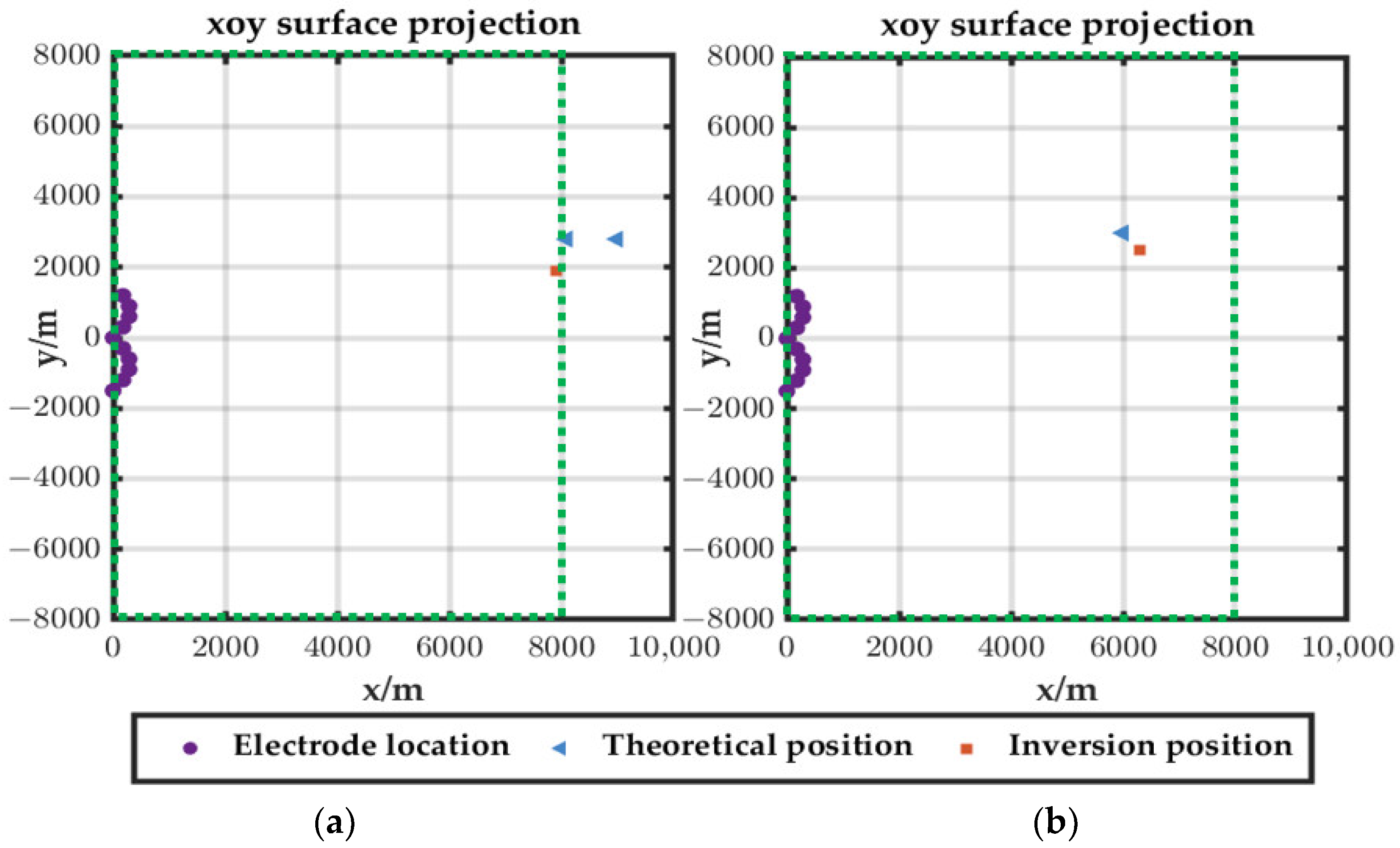
3.2.1. The Influence of Electrode Layout Range

In order to explore the influence of electrode layout range on the positioning results, under different noise conditions, keep the number of electrodes unchanged, change the electrode layout range—that is, change L—and simulate the inversion of field source position, the variation rule of the field source position deviation ${\delta }_{\left|\overline{r}\right|}$ with the electrode layout range can be obtained, as shown in Figure 8. The error band marked in the figure when S = 20 dB is used to indicate the fluctuation range of the data. It can be seen that, under the same other conditions, no matter the noise level, ${\delta }_{\left|\overline{r}\right|}$ shows a decreasing trend with the increase in L.

Figure 9 is the positioning diagram when S = 40 dB and L is replaced by 150 m, 400 m, and 650 m. It is obvious that, under the same noise conditions, with the increase in L, the inversion accuracy and the inversion point aggregation are improved, which shows that the electrode layout area is large and the positioning effect is better. In the figure, the blue dots represent the pre-arranged source positions, the green dots represent the positions of each inversion, the red dots represent the average positions of several inversions, and the purple dots represent the electrode positions. The same applies below.

The electrode layout range significantly impacts the inversion results. Specifically, when the distance between the measuring electrodes is small, the correlation among the scalar potentials obtained at the measuring points intensifies. This, in turn, enhances the correlation among the established equations, thereby increasing the complexity of solving the nonlinear equations. Consequently, the iteration process is prone to converging prematurely to a local optimal solution, ultimately reducing the positioning accuracy. Conversely, when the electrode spacing is increased, the correlation among the equations weakens, leading to more stable calculation results and a higher positioning accuracy.

3.2.2. The Influence of the Number of Electrodes

In order to further analyze the influence of the number of electrodes on the inversion results, the range of the electrodes was kept at 4000 m; that is, the y-axis coordinates of measuring electrodes were evenly distributed in the range of (−2000, 2000) m, the x-axis coordinates were $x=\left|\sin \left(\pi y/2000\right)\times 400\right|$ m, and the z-axis coordinates were randomly distributed in the range of (0, 20) m; the number of electrodes was changed, and five different noise intensity conditions were considered. The proposed BVADE algorithm was used to simulate the inversion of the field source position, and the variation in the source vector diameter deviation with the range of the electrodes was observed. The variation in the source vector diameter deviation ${\delta }_{\left|\overline{r}\right|}$ with the number of electrodes is shown in Figure 10.

It can be seen in the above figure that, when using the data of less than six measuring points for inversion, the positioning deviation is large, and it also exceeds 2% when there is no noise. When the number of electrodes is 5~10, ${\delta }_{\left|\overline{r}\right|}$ gradually decreases to less than 8% with the increase in the number of electrodes under 20 dB noise. Generally speaking, when the number of electrodes exceeds 10, ${\delta }_{\left|\overline{r}\right|}$ tends to decrease and then stabilize with the increase in the number of electrodes.

This conclusion aligns with the fundamental principles underlying the mathematical solution of positioning problems. The number of electrodes employed directly corresponds to the number of equations within the nonlinear system. In theory, assuming the dimensions of the solution space (i.e., the number of parameters to be determined) and the range of the electrode layout remain constant, an insufficient number of equations can compromise the solution’s accuracy. Conversely, while an excessive number of equations may not further enhance the solution’s accuracy, it can lead to increased computational time as the number of equations grows.

The aforementioned results demonstrate that, within a six-dimensional solution space (where the number of parameters to be solved equals six), utilizing 10 to 15 electrodes can yield superior inversion outcomes. Although increasing the number of electrodes may marginally enhance the accuracy in noisy environments, the computational time scales almost linearly with the number of electrodes. Consequently, compared to using a larger number of electrodes, employing 10 to 15 electrodes offers a superior overall performance; specifically, under the condition of maintaining positioning accuracy, it reduces the computational burden and accelerates the positioning speed.

In summary, in terms of positioning speed, the proposed algorithm achieves its first convergence at around 23 evolutionary generations and then gradually stabilizes, reaching a stable state of convergence around 50 generations and thereafter remaining almost unchanged, demonstrating a fast convergence speed overall. In terms of positioning accuracy, the preliminary simulation tests (L = 400 m, 10 electrodes, S = 40 dB) showed that the deviations in vector magnitude and field source intensity vector can be as low as 1.58% and 4.3%, respectively. In extended simulation tests under different parameters (L = 300 m, 15 electrodes, and S = ∞, 20, 30, 40, 60 dB), the deviations in vector magnitude and field source intensity vector did not exceed 7.09% and 5.72%, respectively, indicating that the algorithm can achieve low-error, high-precision positioning under different parameters, demonstrating its universal applicability. In terms of noise immunity, as the focus of this paper was on position localization rather than discrimination of field source strength, and considering the characteristics of practical applications, we primarily investigated the influence of two variables—the electrode deployment range and the number of electrodes—on the positioning accuracy. On the one hand, when the number of electrodes is fixed, the positioning accuracy decreases significantly with the increase in the electrode deployment range. Under low noise levels (S ≥ 40 dB), the positioning accuracy can decrease from approximately 5% for a small deployment range (spacing L ≤ 200 m) to approximately 0.8% for a large deployment range (spacing L ≥ 700 m). Under high noise levels (S < 40 dB), the positioning accuracy can decrease from approximately 9% for a small deployment range (spacing L ≤ 200 m) to 2.5% for a large deployment range (spacing L ≥ 700 m). On the other hand, when the deployment range is fixed, the positioning accuracy decreases significantly with the increase in the number of electrodes. Under low noise levels (S ≥ 40 dB), the positioning accuracy can decrease from approximately 5% for a small number of electrodes (≤10) to approximately 1.3% for a large number of electrodes (≥50). Under high noise levels (S < 40 dB), the positioning accuracy can decrease from approximately 7.2% for a small number of electrodes (≤10) to approximately 3.5% for a large number of electrodes (≥50). This indicates that the choice of electrode deployment range and number has a certain significance for improving positioning accuracy in practical applications. Moreover, regardless of the electrode deployment range and number chosen based on actual conditions, the algorithm can maintain small positioning errors and high positioning accuracy under both low and high noise levels, demonstrating good noise immunity. Based on the simulation test results and summarized patterns, in practical engineering applications using this method, a larger deployment range of sensors and a higher number of sensors within that range will result in higher positioning accuracy. However, it should be noted that the deployment range refers to a relative range, and the specific electrode spacing and deployment range should be determined based on the needs of the specific engineering application. For example, for long-range positioning, the electrode spacing and deployment range should be larger, while for short-range positioning, the deployment range can be relatively smaller.

4. Laboratory Verification of the Positioning Method

In the laboratory, a cuboid pool made of PE plastic with dimensions of 5.0 m × 3.0 m × 0.78 m was used to hold brine to simulate the shallow sea environment, and a solid Ag/AgCl electrode array for determining potential was arranged on the middle line of the pool (set to x = 0 m), as shown in Figure 11. We took the water surface as the xoy plane, the diagonal intersection of the water surface as the origin of the coordinates, and the vertical downward direction as the positive direction of the z-axis. The probe electrode support was 190.0 cm in length, 15.0 cm in width, 2.0 cm in thickness at the bottom, 10.0 cm in height, 1.6 cm in diameter, and 10.0 cm in spacing between holes. In order to prove the effectiveness of the proposed positioning method, platinum plates (analog current elements) were used to locate the underwater vehicle.

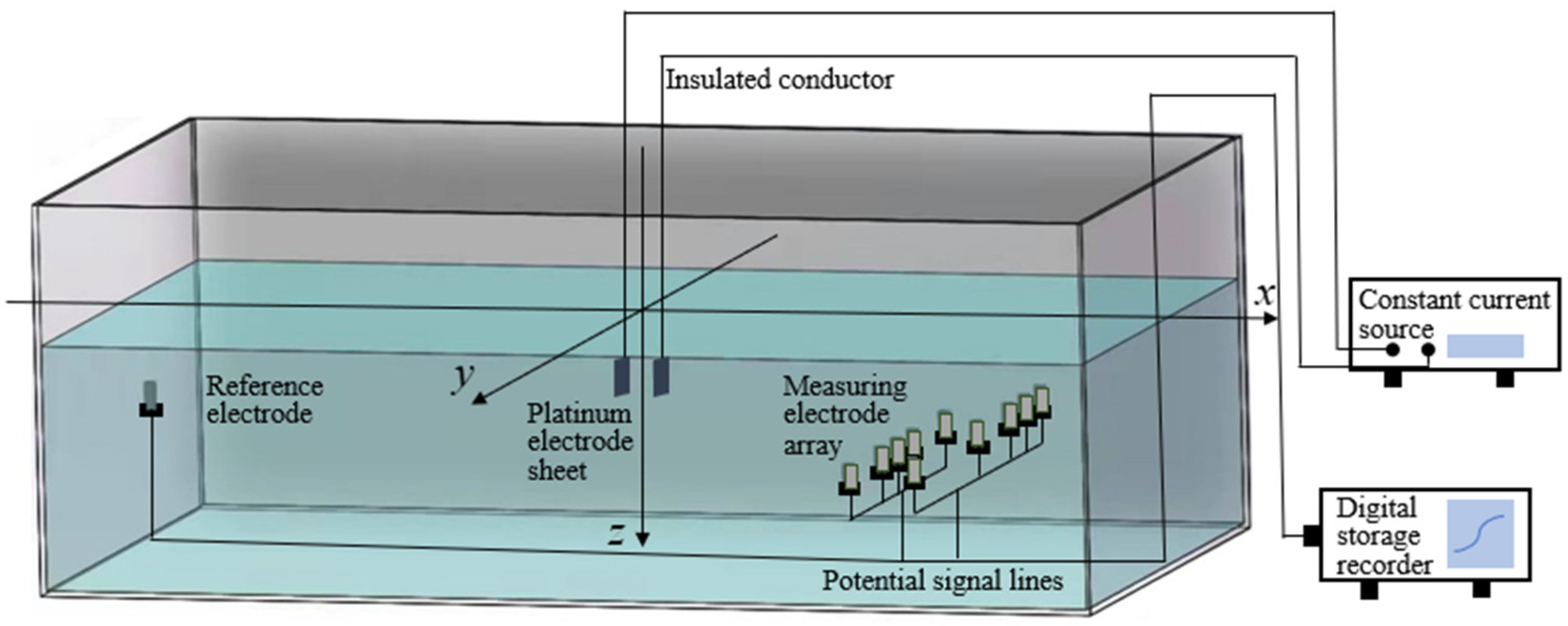
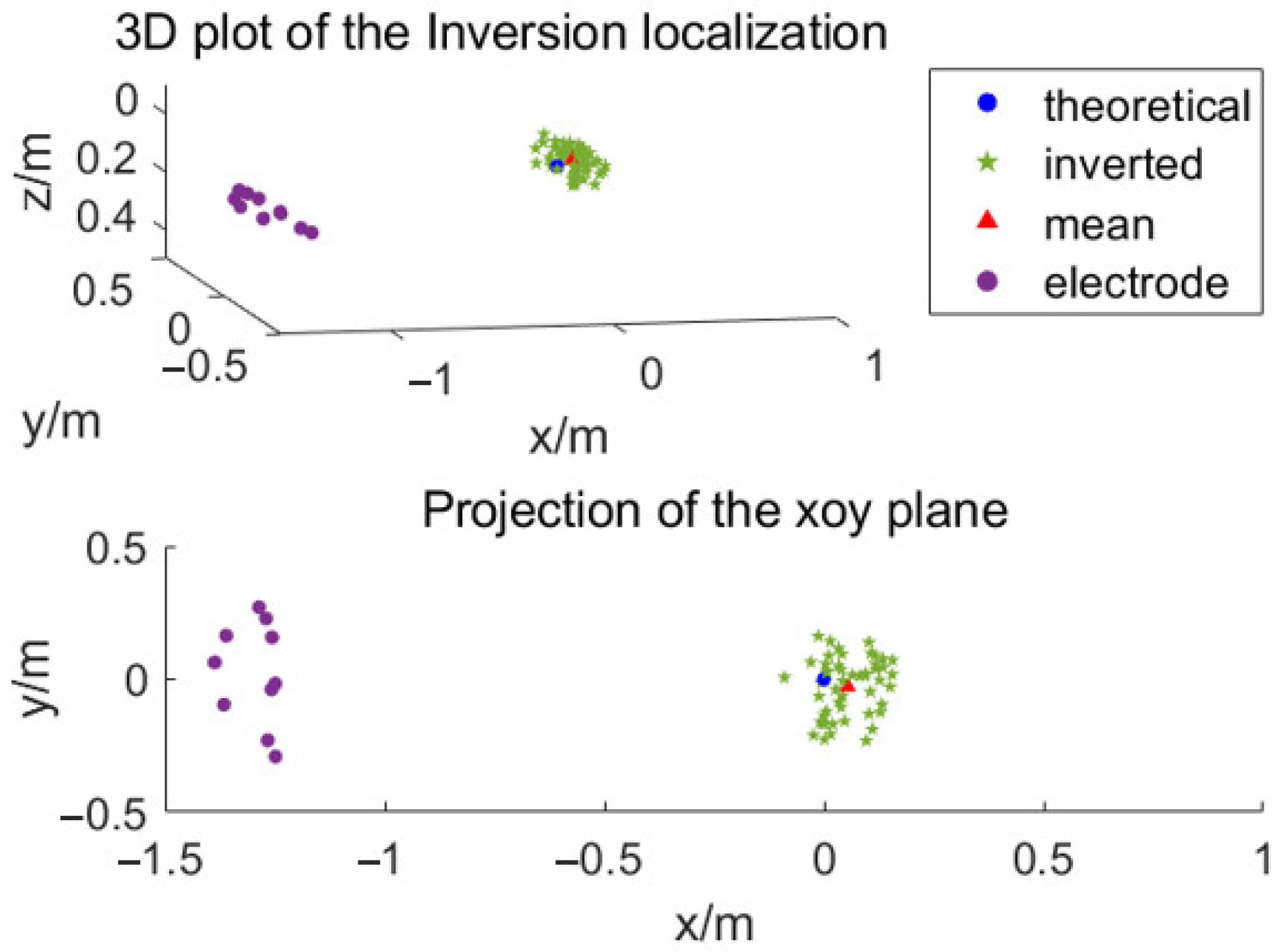
4.1. Current Element Positioning Experiment

Two platinum analog current elements with dimensions of 6.0 mm × 7.0 mm, which were placed in parallel and opposite and set 18.0 mm apart, were supplied by a DC constant current source, I = 500 mA. The simulated seawater conductivity was 0.86 S/m, the simulated seawater depth D was 37.0 cm, and the field source was located 8.5 cm below the water surface. After the analog current element was energized, it moved along the guide rail driven by the slider, and the corresponding potential value was measured synchronously by the probe electrode. After coordinate transformation, the potential distribution of the current element located at (0, 0, 0.085) m and with an intensity of about 0.009 A·m on the depth plane where the probe electrode was located could be obtained. The layout diagram of the field source and detection sensor is shown in Figure 12.

The location of the current element was determined through the utilization of experimental data following coordinate transformation. To invert the parameters of the current element, scalar potential values from 10 randomly selected positions within the measurement area were employed. Subsequently, after conducting 100 inversions, the average value was computed, and the positioning results are presented in

Table 3. Laboratory inversion results.

$\overline{\mathit{r}}/\mathbf{m}$	${\mathit{\delta }}_{\left|\overline{\mathit{r}}\right|}/\%$	$\overline{\mathit{p}}/\mathbf{A}·\mathbf{m}$	${\mathit{\delta }}_{\left|\overline{\mathit{p}}\right|}/\%$
(0.0543, −0.0274, 0.0576)	5.11	(0.0091, −0.0005, 0.0004)	7.2

and Figure 13. In the tables and figures, the theoretical positions are also referred to as the actual laboratory deployment positions. The figures and tables reflect the comparison between the simulated positions obtained through inversion and the theoretical deployment positions.

The deviation of the source radius and source intensity from the measured underwater potential data was 5.11% and 7.20%, respectively. Considering the influence of the boundary effect background noise and spatial position measurement in the experiment, this shows that the current element location in the three-layer parallel stratified sea area model can be completed by using the location method established in this paper.

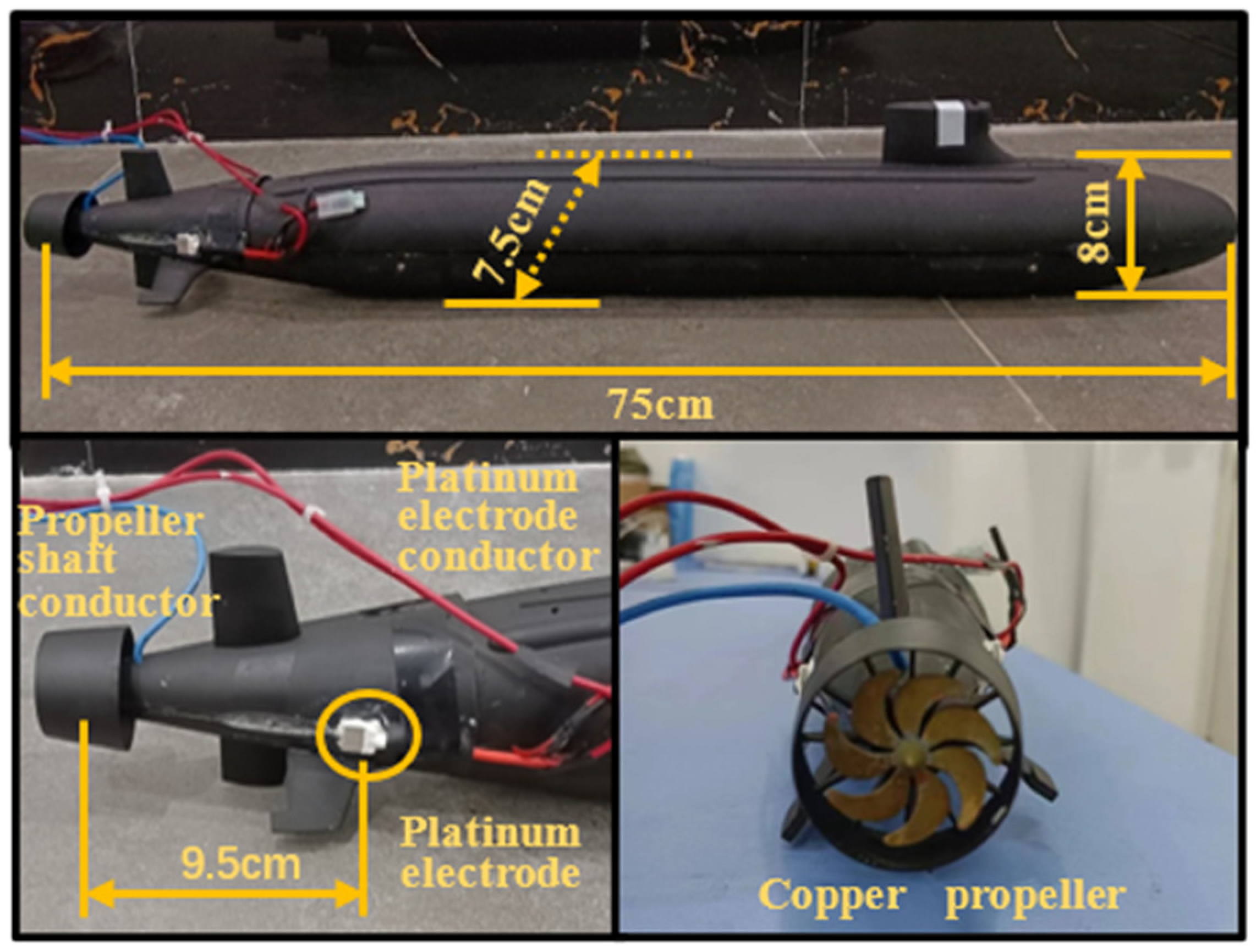
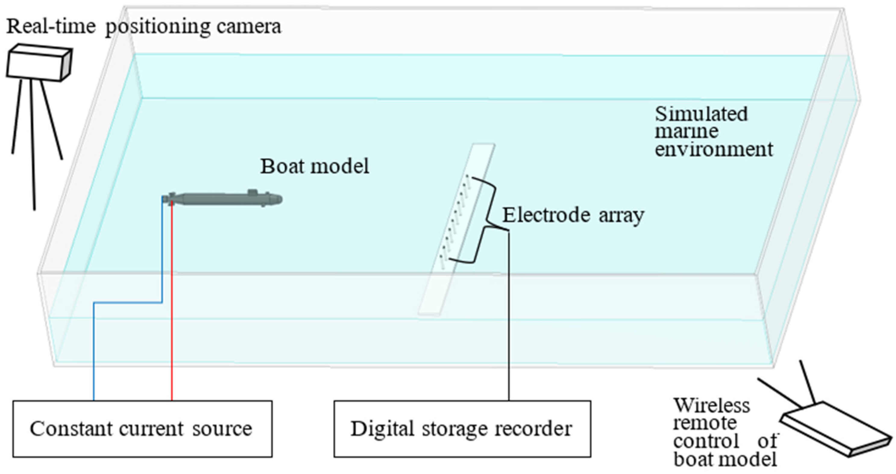
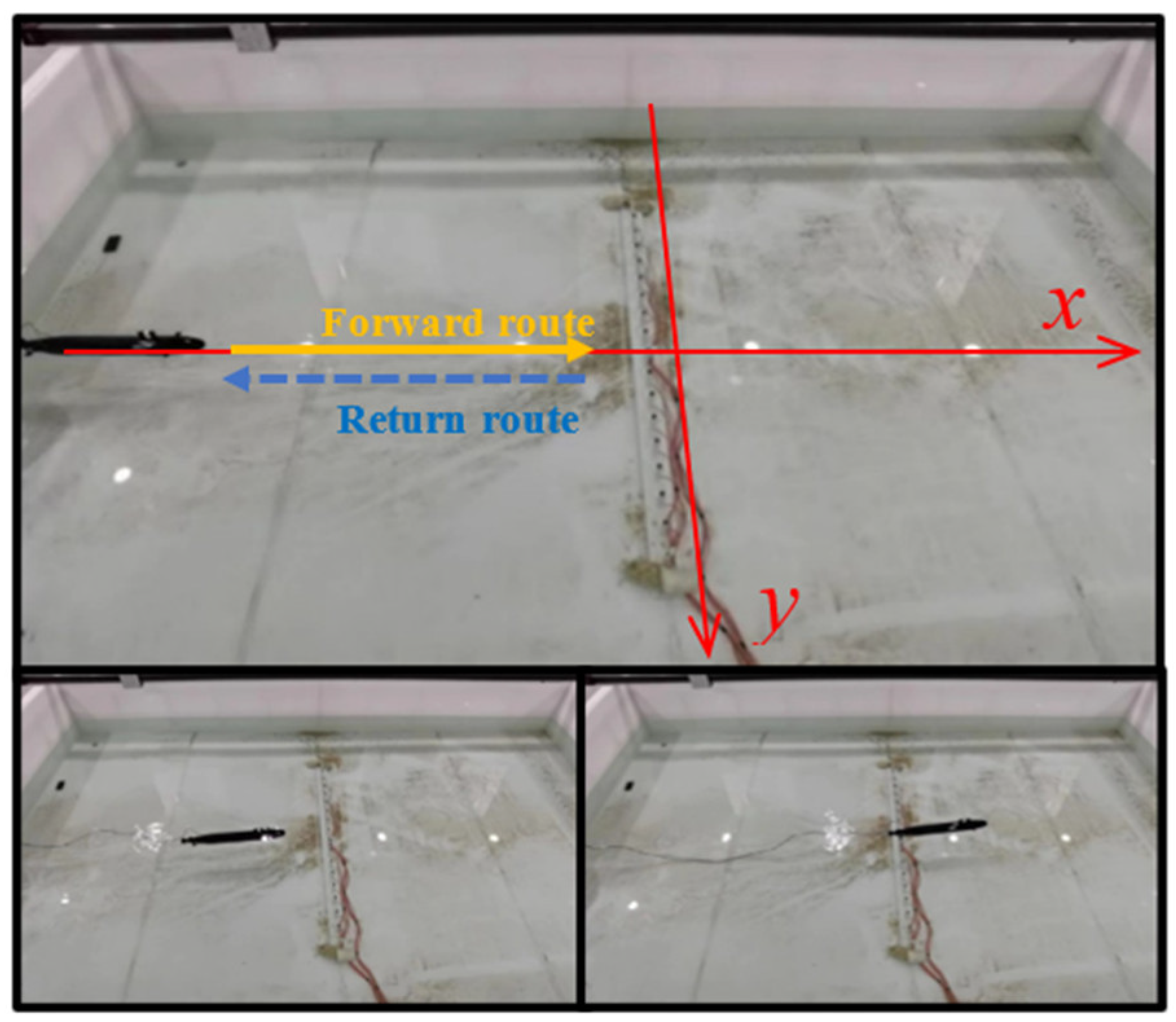
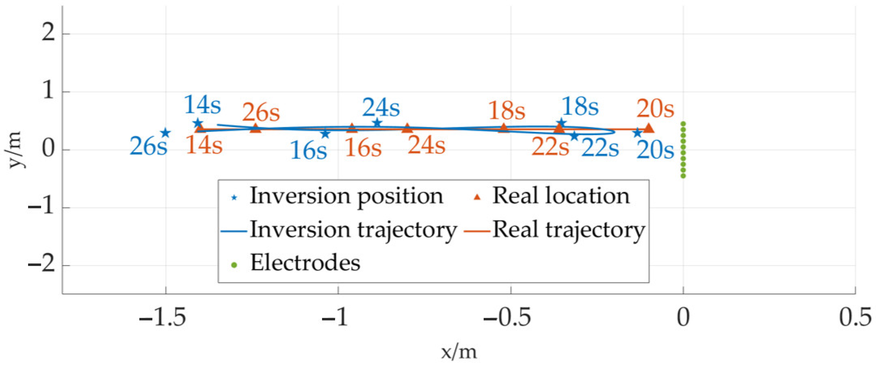
4.2. Positioning Experiment of the Moving Underwater Vehicle

To further validate the applicability of our method in practical engineering, we conducted a continuous positioning experiment using a real submarine model based on the aforementioned positioning experiments with the equivalent field source model. The model used in this experiment is shown in Figure 14.

Figure 14 shows the underwater vehicle model used. The surface of the hull is coated with insulating materials, and the stern of the underwater vehicle is equipped with copper propellers, which are driven by the motor in the underwater vehicle and controlled by wireless remote control. A pair of platinum anodes are arranged in parallel near both sides of the propeller (the dimensions of the two anodes are 6.0 mm × 7.0 mm × 0.3 mm, the distance is 5.5 cm, and the vertical distance between the centerline and the propeller plane is 9.5 cm). The platinum anode is connected to the positive electrode of the external constant current source, and the propeller drive shaft is connected to the negative electrode of the constant current source. Therefore, when electrified, the current consists of the positive electrode of the constant current source → platinum anode → seawater → propeller → shaft → negative electrode of the constant current source, which constitutes the ICCP (impressed current cathodic protection) system of the underwater vehicle and provides a cathodic protection current for the underwater vehicle. In order to calibrate the position and speed of the underwater vehicle, the camera is used to record the position of the field source in real time. The layout diagram of the whole experimental device is shown in Figure 15. The electrode array was deployed at the symmetrical position in the middle of the water area, and the model was also moved according to the symmetry axis of the experimental environment, ensuring the symmetry of the entire experimental setup. The simulated seawater depth and conductivity were the same as before, and the anode sheet on the underwater vehicle was kept at 10.0 cm below the water surface.

After the ICCP system of the underwater vehicle was electrified and stabilized, we drove the underwater vehicle remotely, traveling from the negative to the positive direction of the x-axis along the center line of the pool and controlling it to return according to the original path when the propeller crossed directly above the electrode array, as shown in Figure 16. The potential of each measuring electrode was recorded synchronously with a digital storage recorder, and after the range of each electrode pair was removed, the potential measurement value of each measuring point was obtained. In the experiment, the current of ICCP system was set to 0.3 A, and 10,896 potential signals of 16 groups were collected after sailing for 34 s.

In order to reduce the influence caused by the boundary of the water tank’s wall, the test data of 10 electrodes in the middle of the detection array were selected during positioning, and the track area of the underwater vehicle was limited to x ∈ [−1.8, −0.2] m. By recording the position and time of the underwater vehicle in the round-trip phase with a real-time recording camera, the average speed of the underwater vehicle was 0.2199 m/s, and the real position corresponding to each time of the underwater vehicle was obtained.

Using the aforementioned positioning method, the continuous positioning of the submarine model was achieved. The positioning result data and the corresponding schematic diagram of the submarine model’s trajectory positioning are shown in

Table 4. Inversion results of the underwater vehicle track.

Moment/s	Theoretical Position/m	Actual Location/m	Absolute Deviation/m
14	(−1.4, 0.36, 0.1)	(−1.41, 0.47, 0.09)	0.11
16	(−0.96, 0.36, 0.1)	(−1.04, 0.28, 0.10)	0.11
18	(−0.52, 0.36, 0.1)	(−0.35, 0.46, 0.10)	0.20
20	(−0.1, 0.36, 0.1)	(−0.13, 0.29, 0.09)	0.07
22	(−0.36, 0.36, 0.1)	(−0.31, 0.23, 0.09)	0.14
24	(−0.80, 0.36, 0.1)	(−0.89, 0.47, 0.09)	0.14
26	(−1.24, 0.36, 0.1)	(−1.50, 0.29, 0.10)	0.27

and Figure 17, respectively. These illustrate the difference in data between the target model’s movement position recorded by the high-speed camera and the simulated position derived from the positioning algorithm, as well as the intuitive display on the schematic diagram.

Considering the influence of limited experimental waters and the poor stability of the underwater vehicle’s round-trip motion, it can be seen in Table 4 and Figure 17 that the positioning track of the underwater vehicle is in good agreement with the actual track, and the inversion positioning error at each point along the almost 3-meter-long back-and-forth path is within the range of [0.07, 0.27] m. After calculation, the average positioning distance error is only 0.148 m. This level of accuracy, considering various uncertain error factors (such as manual operations), sufficiently demonstrates the effectiveness of the positioning method in the experiment, which shows that the positioning method established in this paper has a good practicability.

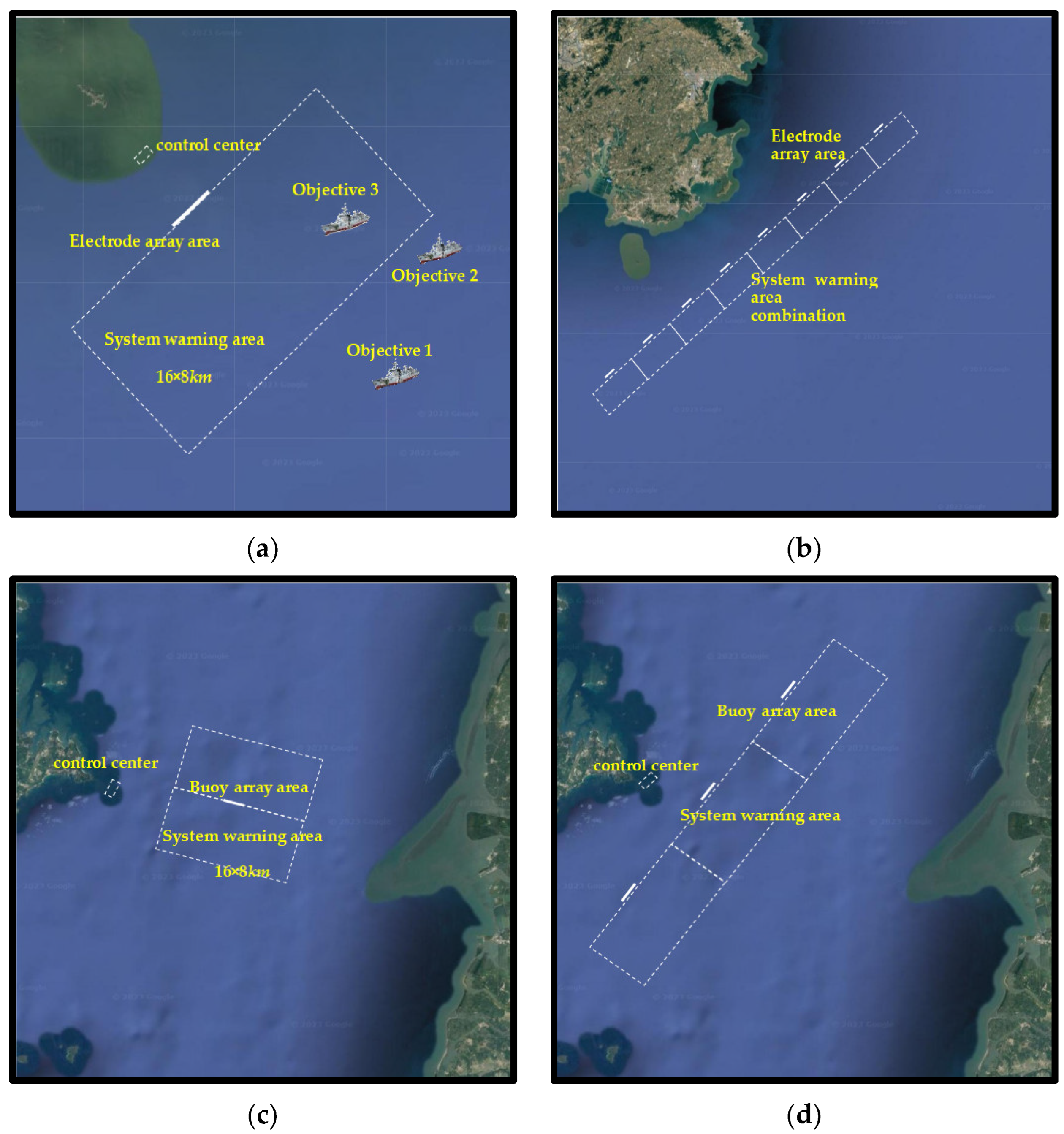
4.3. Discussion and Prospects of Practical Application Scenarios

Firstly, the positioning method proposed in this paper covers the entire search area and does not impose requirements on the location or direction of the field source. Meanwhile, for the practical application scenario of passive warning for unknown underwater vehicles, the appearance of underwater vehicles in the ocean is often random in both location and direction. The direction of the equivalent field source is closely related to the moving direction of the target’s body, and its intensity is related to the target’s size and anti-corrosion materials. Therefore, the positioning method and algorithm need to be insensitive to the orientation and movement direction of the target. Combining the characteristics of the aforementioned positioning method and the usage features of underwater vehicle positioning and warning, we believe that the proposed method can be applied to two passive warning positioning application scenarios: shore-based warning and buoy-based warning. Both are suitable for shallow sea areas and are feasible under conditions of shallow water where sensors are easily deployed, as well as challenging seabed operations where sensors are difficult to deploy. The deployment methods can be submerged, floating, or semi-submerged. The overall idea is to utilize a pre-deployed electrode array to capture underwater electric field signals, and then utilize a computing unit to invert the position parameters of the underwater vehicle in order to determine whether the target is within the warning range. From the perspective of practical warning applications, this is a very valuable approach worth considering.

Figure 18 depicts the configurations for single shore-based warning (a), combined shore-based warning (b), single buoy-based warning (c), and combined buoy-based warning (d) in a certain sea area with a water depth of 70 m. The horizontal distance between the detection electrodes, L, is 300 m, and 10 electrodes are distributed in the white solid region shown in the figure, which represents the array sensor deployment area. The combined warning approach can significantly increase the warning area coverage. The sizes of the various regions in the figure are drawn in equal proportion to the map. The warning system primarily consists of underwater detection electrode arrays, signal transmission units, computing units, control units, and other components. These work together to accomplish the functions of scalar potential detection, signal conditioning, parameter inversion, and alert notification, enabling the positioning, warning, and surveillance of underwater vehicles invading the rectangular dashed-line area.

Regarding the warning strategy, when the system is on alert, the target determination falls into three scenarios:

① If the target has not entered the warning area, as shown by Objective 1 in Figure 18a, the target is still far away from the detection electrodes, and the system is unable to capture the potential signal generated by the target and, thus, unable to invert the target’s position.

② If the target has not entered the warning area, as shown by Objective 2 in Figure 18a, the target is not too far from the detection electrodes, and the system is able to collect the weak electric field signal that it generates. However, the inverted position has exceeded the algorithm’s search area (i.e., the warning area, the rectangular region formed by the white dashed lines set earlier). When the algorithm iterates to calculate the target’s position, it will no longer be the actual position but a certain point on the boundary of the warning area. The proof is as follows:

At this time, during the iteration process of the algorithm, the objective function is actually

$${f^{\prime }}_k=\frac{\mathit{p}·{\overline{\mathit{R}}}_k}{4\pi \sigma {\left|{\overline{\mathit{R}}}_k\right|}^3}+\frac{\mathit{p}\mathit{Q}·{\overline{{\mathit{R}}^{\prime }}}_k}{4\pi \sigma {\left|{\overline{{\mathit{R}}^{\prime }}}_k\right|}^3}-{\phi }_k^m,$$

(30)

where ${\overline{\mathit{R}}}_k=(x_k-{x^{\prime }}_0,y_k-{y^{\prime }}_0,z_k-{z^{\prime }}_0)$, ${\overline{\mathit{R}}}_k\prime =(x_k-{x^{\prime }}_0,y_k-{y^{\prime }}_0,z_k+{z^{\prime }}_0)$, and theoretically, ${\phi }_k^m=\frac{\mathit{p}·{\mathit{R}}_k}{4\pi \sigma {\left|{\mathit{R}}_k\right|}^3}+\frac{\mathit{p}\mathit{Q}·{{\mathit{R}}^{\prime }}_k}{4\pi \sigma {\left|{{\mathit{R}}^{\prime }}_k\right|}^3}$, while $f^{\prime }$ represents the actual objective function. Substituting this into the previous equation provides the following:

$${f^{\prime }}_k=\frac{\mathit{p}·{\overline{\mathit{R}}}_k}{4\pi \sigma {\left|{\overline{\mathit{R}}}_k\right|}^3}+\frac{\mathit{p}\mathit{Q}·{\overline{{\mathit{R}}^{\prime }}}_k}{4\pi \sigma {\left|{\overline{{\mathit{R}}^{\prime }}}_k\right|}^3}-(\frac{\mathit{p}·{\mathit{R}}_k}{4\pi \sigma {\left|{\mathit{R}}_k\right|}^3}+\frac{\mathit{p}\mathit{Q}·{{\mathit{R}}^{\prime }}_k}{4\pi \sigma {\left|{{\mathit{R}}^{\prime }}_k\right|}^3})$$

(31)

Since the target is outside the warning zone, while ${{\mathrm{M}}^{\prime }}_0({x^{\prime }}_0,{y^{\prime }}_0,{z^{\prime }}_0)$ is within the warning zone, based on the approach of minimizing a function, the algorithm will strive to find a value of ${{\mathrm{M}}^{\prime }}_0$ that minimizes ${f^{\prime }}_k$ in Equation (31). In solving a single-target problem, when $\mathit{p}$ remains constant, ${f^{\prime }}_k$ will only be smaller if ${{\mathrm{M}}^{\prime }}_0$ is closer to ${\mathrm{M}}_0$. Therefore, the theoretical position of ${{\mathrm{M}}^{\prime }}_0$ is at the closest point on the outer edge of the warning zone to ${\mathrm{M}}_0$. As a result, the system inverts the target’s position to the boundary of the search area, as illustrated in Figure 19a. The theoretical positions of the targets in the figure are (8100, 2800, 70) and (9000, 2800, 70), both of which lie outside the system’s warning zone. As evident from the figure, the inverted positions are all situated on the perimeter of the warning zone.

③ If the target enters the warning area, as shown by Objective 3 in Figure 18a, the system is able to capture the electric field signal generated by the target and accurately calculate its position, as illustrated in Figure 19b.

Regarding the warning process, as illustrated in Figure 20, it can be divided into three parts:

① Under daily monitoring conditions, the ground control center conducts surveillance, with the detection electrodes continuously attempting to capture weak potential signals in the sea area. After filtering and amplifying the signals, if no valuable potential signals can be extracted, this proves that there are no incoming underwater vehicle targets within the detection warning range, and the system continues to monitor the area.

② If valuable potential signals can be extracted, they are sent to the computing unit for inverting the target position. If the target is located at the boundary of the warning area, this indicates that an enemy underwater vehicle or submarine target has been detected but has not yet entered the warning area, allowing the system to continue with its daily monitoring.

③ If the inverted target is located within the warning area, this indicates that an incoming target has entered the warning area, triggering the system alarm, allowing for subsequent actions to be implemented accordingly.

Since the warning system is a practical application designed based on the studied passive electric field target localization method, theoretically, it has no specific requirements for the incoming direction of the target or the direction of the field source intensity. However, in the algorithm calculations, we must set a certain computational domain, and the typically chosen calculation range is often larger than our expected warning area. However, in practical applications, there are no boundary limitations in any x, y, or z direction. As for incoming targets near the boundary, whether or not the special angle of their direction and the different field source intensity directions caused by the vehicle’s body posture will affect the positioning accuracy requires further investigation. This serves as a future outlook for the work presented in this section.

5. Conclusions

To fulfill the practical application demands of underwater vehicle passive electric field localization technology, this paper introduces a scalar-potential-based method for underwater vehicle passive electric field positioning. This method leverages the intelligent differential evolution algorithm and is suitable for a three-layer stratified marine environment. Firstly, the positioning mathematical model was formulated based on the scalar potential distribution law of current elements in the stratified marine setting. An objective function was chosen, and the positioning problem was recast as the minimization of this objective function. Secondly, given the differential evolution algorithm’s weak initial-value dependence, it was chosen as the foundation for the localization algorithm. To enhance the algorithm’s performance, avoid local optima, and improve convergence, a parameter-adaptive strategy, along with a boundary mutation processing mechanism, was introduced to enhance the performance of the algorithm. The simulation results demonstrate the algorithm’s high inversion accuracy, robust noise resistance, and broad applicability; additionally, they indicate that the proposed positioning method has no specific requirements for sensor measurement configurations, although a wide range and moderate number of sensors can enhance the electric field positioning effectiveness for shallow-water underwater vehicles. Finally, laboratory experiments were conducted to localize underwater simulated current elements and underwater vehicle tracks. The results indicate that the proposed positioning method fulfills the requirements of independent initial values, excellent noise resistance, fast positioning speed, ease of implementation, and adaptability in shallow-water environments, thereby exhibiting strong practical application potential.

References

1. Smith, T.A.; Rigby, J. Underwater Radiated Noise from Marine Vessels: A Review of Noise Reduction Methods and Technology. Ocean. Eng. 2022, 266, 112863. [Google Scholar] [CrossRef]
2. Jin, H. Underwater Target Localization and Inversion Technology Based on Magnetic Anomaly Detection. Ph.D. Thesis, Nanjing University of Science & Technology, Nanjing, China, 2022. Available online: https://link.oversea.cnki.net/doi/10.27241/d.cnki.gnjgu.2022.000073 (accessed on 10 December 2023).
3. Han, R. Development of several key technologies and equipment for high-power and wide-band digital power amplifier. Ph.D. Thesis, Hunan University, Changsha, China, 2022. Available online: https://link.oversea.cnki.net/doi/10.27135/d.cnki.ghudu.2022.000207 (accessed on 3 March 2024).
4. Zhang, J.; Yu, P.; Jiang, R.; Xie, T. Real-Time Localization for Underwater Equipment Using an Extremely Low Frequency Electric Field. Def. Technol. 2022, 26, 203–212. [Google Scholar] [CrossRef]
5. Wang, X.; Zhang, J.; Xu, Q. Influence of mass transfer process on ship electric fieldunder laminar flow condition. J. Nav. Univ. Eng. 2020, 32, 1–6+14. Available online: https://link.oversea.cnki.net/doi/10.7495/j.issn.1009-3486.2020.02.001 (accessed on 1 November 2023).
6. Kato, R.; Takahashi, M.; Ishii, N.; Chen, Q.; Yoshida, H. Investigation of a 3-D Undersea Positioning System Using Electromagnetic Waves. IEEE Trans. Antennas Propagat. 2021, 69, 4967–4974. [Google Scholar] [CrossRef]
7. Duecker, D.-A.; Geist, A.; Hengeler, M.; Kreuzer, E.; Pick, M.-A.; Rausch, V.; Solowjow, E. Embedded Spherical Localization for Micro Underwater Vehicles Based on Attenuation of Electro-Magnetic Carrier Signals. Sensors 2017, 17, 959. [Google Scholar] [CrossRef] [PubMed]
8. Mohd Aris, M.N.; Daud, H.; Mohd Noh, K.A.; Dass, S.C. Stochastic Process-Based Inversion of Electromagnetic Data for Hydrocarbon Resistivity Estimation in Seabed Logging. Mathematics 2021, 9, 935. [Google Scholar] [CrossRef]
9. Li, R.; Di, Y.; Zuo, Q.; Tian, H.; Gan, L. Enhanced Whale Optimization Algorithm for Improved Transient Electromagnetic Inversion in the Presence of Induced Polarization Effects. Mathematics 2023, 11, 4164. [Google Scholar] [CrossRef]
10. Conde Mones, J.J.; Hernández Gracidas, C.A.; Morín Castillo, M.M.; Oliveros Oliveros, J.J.; Juárez Valencia, L.H. Stable Numerical Identification of Sources in Non-Homogeneous Media. Mathematics 2022, 10, 2726. [Google Scholar] [CrossRef]
11. Chen, C.; Yang, J.; Du, C.; Si, L. Distribution Features of Underwater Static Electric Field Intensity of Ship in Typical Restricted Sea Areas. Prog. Electromagn. Res. C 2020, 102, 225–240. [Google Scholar] [CrossRef]
12. Shang, W.; Xue, W.; Li, Y.; Wu, X.; Xu, Y. An Improved Underwater Electric Field-Based Target Localization Combining Subspace Scanning Algorithm And Meta-EP PSO Algorithm. JMSE 2020, 8, 232. [Google Scholar] [CrossRef]
13. Reznichenko, I.; Podržaj, P.; Peperko, A. Calculation of Stationary Magnetic Fields Based on the Improved Quadrature Formulas for a Simple Layer Potential. Mathematics 2023, 12, 21. [Google Scholar] [CrossRef]
14. Wu, C.; Zhao, S. Study on the localization of the dectric dipole sources. J. Phys. 2007, 56, 5180–5184. Available online: https://link.oversea.cnki.net/doi/10.3321/j.issn:1000-3290.2007.09.030 (accessed on 31 August 2023).
15. Samann, F.; Rausch, A.; Schanze, T. Electrical Dipole Source Localization Using Hybrid Least Squares Method in Combination with ICA. Curr. Dir. Biomed. Eng. 2019, 5, 361–363. [Google Scholar] [CrossRef]
16. Ci, L.; Xue, W.; Dang, J.; Jia, P.; Xu, Y.; Gao, J. Underwater Target Electric Field Location Algorithm Based on Electric Dipole. In Proceedings of the IEEE Asia-Pacific Conference on Image Processing, Electronics and Computers, Dalian, China, 14–16 April 2022; pp. 222–227. [Google Scholar] [CrossRef]
17. Liu, Z.; Gao, J.; Xu, L.; Jia, P.; Pan, D.; Xue, W. Electromagnetic Fusion Underwater Positioning Technology Based on ElasticNet Regression Method. In Proceedings of the 2022 IEEE 10th International Conference on Information, Communication and Networks (ICICN); IEEE, Zhangye, China, 23 August 2022; pp. 121–126. [Google Scholar] [CrossRef]
18. Du, C.; Chen, C.; Huang, G. Study on location method of electric dipole source in parallel stratified sea area. J. Electron. 2021, 49, 1761–1767. Available online: https://link.oversea.cnki.net/doi/10.12263/DZXB.20200356 (accessed on 30 August 2023).
19. Wang, C.; Xu, Y.; Qi, J.; Shang, W.; Liu, M.; Chen, W. Passive Electromagnetic Field Positioning Method Based on BP Neural Network in Underwater 3-D Space. In Advanced Hybrid Information Processing; Liu, S., Ma, X., Eds.; Lecture Notes of the Institute for Computer Sciences, Social Informatics and Telecommunications Engineering; Springer International Publishing: Cham, Switerland, 2022; Volume 416, pp. 292–304. ISBN 978-3-030-94550-3. [Google Scholar] [CrossRef]
20. Hou, M.; Wu, H.; Peng, J.; Li, K. Long-Range and High-Precision Localization Method for Underwater Bionic Positioning System Based on Joint Active–Passive Electrolocation. Sci. Rep. 2023, 13, 21475. [Google Scholar] [CrossRef] [PubMed]
21. Chen, C.; Wu, X.; Yang, J.; Sun, J. Method for Detecting Electrical Interface in Sea Area Based on Active Electric Field. J. Phys. Conf. Ser. 2023, 2419, 012032. [Google Scholar] [CrossRef]
22. Xu, Y.; Xue, W.; Li, Y.; Guo, L.; Shang, W. Multiple Signal Classification Algorithm Based Electric Dipole Source Localization Method in an Underwater Environment. Symmetry 2017, 9, 231. [Google Scholar] [CrossRef]
23. Xu, Y. Research on Electric Field Location Technology of Underwater Target Based on Optimization Theory. Ph.D. Thesis, Harbin Engineering University, Harbin, China, 2018. [Google Scholar]
24. Chew, W. A quick way to approximate a Sommerfeld-Weyl-type integral (antenna far-field radiation). IEEE Trans. Antennas Propag. 1988, 36, 1654–1657. [Google Scholar] [CrossRef]
25. Dvorak, S. Application of the fast Fourier transform to the computation of the Sommerfeld integral for a vertical electric dipole above a half-space. IEEE Trans. Antennas Propag. 1992, 40, 798–805. [Google Scholar] [CrossRef]
26. Deng, W.; Shang, S.; Cai, X.; Zhao, H.; Song, Y.; Xu, J. An Improved Differential Evolution Algorithm and Its Application in Optimization Problem. Soft Comput. 2021, 25, 5277–5298. [Google Scholar] [CrossRef]
27. Zhao, J.; Zhang, B.; Guo, X.; Qi, L.; Li, Z. Self-Adapting Spherical Search Algorithm with Differential Evolution for Global Optimization. Mathematics 2022, 10, 4519. [Google Scholar] [CrossRef]
28. Li, Y.; Wang, S.; Yang, B. An Improved Differential Evolution Algorithm with Dual Mutation Strategies Collaboration. Expert Syst. Appl. 2020, 153, 113451. [Google Scholar] [CrossRef]
29. Tan, Z.; Li, K.; Wang, Y. Differential Evolution with Adaptive Mutation Strategy Based on Fitness Landscape Analysis. Inf. Sci. 2021, 549, 142–163. [Google Scholar] [CrossRef]
30. Tan, Z.; Li, K. Differential Evolution with Mixed Mutation Strategy Based on Deep Reinforcement Learning. Appl. Soft Comput. 2021, 111, 107678. [Google Scholar] [CrossRef]
31. Xia, X.; Gui, L.; Zhang, Y.; Xu, X.; Yu, F.; Wu, H.; Wei, B.; He, G.; Li, Y.; Li, K. A Fitness-Based Adaptive Differential Evolution Algorithm. Inf. Sci. 2021, 549, 116–141. [Google Scholar] [CrossRef]
32. Mai, W.; Liu, W.; Zhong, J. Adaptive Differential Evolution Algorithm Based on Population State Information. J. Commun. 2023, 44, 34–46. [Google Scholar]
33. Abdel-Basset, M.; Mohamed, R.; Hezam, I.M.; Alshamrani, A.M.; Sallam, K.M. An Efficient Evolution-Based Technique for Moving Target Search with Unmanned Aircraft Vehicle: Analysis and Validation. Mathematics 2023, 11, 2606. [Google Scholar] [CrossRef]
34. Boks, R.; Kononova, A.V.; Wang, H. Quantifying the Impact of Boundary Constraint Handling Methods on Differential Evolution. In Proceedings of the Genetic and Evolutionary Computation Conference Companion, Lille, France, 7 July 2021; pp. 1199–1207. [Google Scholar] [CrossRef]
35. Stanovov, V.; Semenkin, E. Adaptation of the Scaling Factor Based on the Success Rate in Differential Evolution. Mathematics 2024, 12, 516. [Google Scholar] [CrossRef]
Figure 1. Positioning field model.
Mathematics 12 01832 g001
Figure 2. Simulation diagram of the change in κ . (a) Simulation results at a depth of D = 1000 m; (b) Simulation results at a depth of D = 500 m; (c) Simulation results at a depth of D = 250 m.
Mathematics 12 01832 g002
Figure 3. Boundary mutation processing flowchart.
Mathematics 12 01832 g003
Figure 4. BVADE algorithm flowchart.
Mathematics 12 01832 g004
Figure 5. The simulation results of the BVADE algorithm.
Mathematics 12 01832 g005
Figure 6. Test results of the convergence speed of the BVADE algorithm.
Mathematics 12 01832 g006
Figure 7. Electrode array configuration.
Mathematics 12 01832 g007
Figure 8. Variation in δ r ¯ with L.
Mathematics 12 01832 g008
Figure 9. Inversion of the location map under 40 dB noise when L = 150 m (a), 400 m (b), and 650 m (c).
Mathematics 12 01832 g009
Figure 10. Variation in δ r ¯ with the number of electrodes.
Mathematics 12 01832 g010
Figure 11. Experimental pool.
Mathematics 12 01832 g011
Figure 12. Schematic diagram of the field source and detection sensor layout.
Mathematics 12 01832 g012
Figure 13. Laboratory positioning results.
Mathematics 12 01832 g013
Figure 14. Experimental model of the underwater vehicle.
Mathematics 12 01832 g014
Figure 15. Schematic diagram of the experimental device layout.
Mathematics 12 01832 g015
Figure 16. Underwater vehicle model route map.
Mathematics 12 01832 g016
Figure 17. Underwater vehicle model track inversion positioning map.
Mathematics 12 01832 g017
Figure 18. Schematic diagram of four early warning methods in a certain sea area. (a) single shore-based warning; (b) combined shore-based warning; (c) single buoy-based warning; (d) combined buoy-based warning.
Mathematics 12 01832 g018
Figure 19. Warning simulation scenario diagram. (a) Target is not in the perimeter. (b) Target has entered the perimeter.
Mathematics 12 01832 g019
Figure 20. Early warning process.
Mathematics 12 01832 g020