Group Decision-Making Method with Incomplete Intuitionistic Fuzzy Soft Information for Medical Diagnosis Model

Abstract

The medical diagnosis of many critical diseases is difficult as it usually requires the combined effort of several doctors. At this time, the process of medical diagnosis is actually a group decision-making (GDM) problem. In group medical diagnosis, considering doctors’ weight information and fusing the interaction relation of symptoms remain open issues. To address this problem, a group decision-making method for intuitionistic fuzzy soft environments is proposed for medical diagnosis because the intuitionistic fuzzy soft set (IFSS) integrates the advantages of the soft set and intuitionistic fuzzy set (IFS). Intuitionistic fuzzy soft weighted Muirhead mean operators are constructed by combining Einstein operations with the Muirhead mean (MM) operator, and some properties and results are revealed. A group medical diagnosis model with unknown doctor weight information and incomplete intuitionistic fuzzy soft information is proposed. Similarity measures of the intuitionistic fuzzy soft matrix (IFSM) given by the doctors are used to estimate the incomplete information. To take into account the advantages of objective weight and subjective weight, the combined weights of doctors are calculated based on the IFSMs’ similarity measure and doctors’ grades. The developed operators are then used to combine the evaluation information and handle the correlation of input arguments in the group medical diagnosis process. Finally, a numerical problem is selected to illustrate the superiority of the proposed approach compared to related methods. The combined weights are determined to overcome the shortcomings of the single-weight method to some extent. Meanwhile, the proposed method is more comprehensive, and can provide more flexible and reasonable choices for group medical diagnosis problems.

1. Introduction

Medical diagnosis is a process that directly affects people’s health and lives. One main task in medical science is to obtain an accurate diagnosis [1]. Many scholars have conducted extensive research to find suitable methods for improving the accuracy of medical diagnosis [2,3,4,5,6]. Medical diagnosis for critical diseases is a complex decision-making problem that contains a great deal of symptom analysis. Therefore, a doctor may find it difficult to draw firm conclusions about such diseases without the assistance of their colleagues when assessing the health problem and providing precise diagnosis [7]. Therefore, medical diagnosis is a group decision-making (GDM) problem [8,9]. Two main problems in the GDM process must be solved: one is obtaining evaluation information, that is, weights and evaluation values, and the other is selecting an appropriate method for aggregating this information [10].

In the real world, this may be difficult as people may not be able to provide accurate evaluation values in complex decision-making environments. Generally, the inherent uncertainty in patient history and current signs and symptoms may make it difficult to find the precise diagnosis [11]. As an extension of the fuzzy set (FS) [12], the intuitionistic fuzzy set (IFS) can better describe the complexity and fuzziness of information that contains membership, non-membership, and hesitation information [13]. Medical diagnosis models based on FS theory have been widely investigated. Li et al. applied an approach to medical diagnosis using fuzzy soft sets [14]. Based on the ambiguity measure and Dempster–Shafer theory of evidence, a decision-making method was presented and applied to medical diagnosis [15]. Xiao utilized a hybrid method based on fuzzy soft sets to address medical diagnoses [16]. Thao et al. proposed the concept of a divergence measure of picture fuzzy sets and a new multi-criteria decision-making algorithm for medical diagnosis [17]. An algorithm for medical diagnosis using score matrices has been proposed [18]. For a double-hierarchy hesitant fuzzy linguistic environment, Zhang et al. proposed novel correlation measures for medical diagnoses in Chinese medicine [19]. The theory of fuzzy soft matrices has also been applied in medical diagnosis [20]. Farhadinia developed a divergence-based medical decision-making process for COVID-19 diagnosis in a hesitant fuzzy environment [21]. A novel algorithm for the decision-making problem of neutrosophic soft sets was proposed and applied to medical diagnosis [22]. Considering FS theory’s inherent difficulties and the inadequacy of the parametrization tool, Molodtsov put forward the concept of the soft set [23]. Parameterization in soft set theory is expressed with the aid of words, sentences, and other forms. It is difficult to provide preferences appropriately and accurately using soft sets in uncertain situations. Maji et al. established an intuitionistic fuzzy soft set (IFSS) that integrates the advantages of soft sets and IFSs [24]. Evaluation values in the form of IFSSs can help achieve appropriate results closer to the actual reality because IFSSs can describe decision-makers’ positive, negative, and hesitant traits. The IFSS theory has been further developed. Fuzzy information measures, which include distance measures and fuzzy entropy [25,26], similarity measures [27,28], and correlation coefficients [29], have been widely used in medical diagnosis, pattern recognition, cluster analysis, decision analysis, and other fields. Furthermore, the approximation ideal solution (TOPSIS method) [29], ranking priority relation (PROMETHE) [30], and prospect theory [31] have been developed to deal with practical problems with intuitionistic fuzzy soft information.

Aggregation of information and preferences in the GDM process is important. Various aggregation operators, which are mathematical tools for combining information, have been constructed to combine decision information in different situations. To express information more clearly and elaborately, Seikh and Mandal defined the p,q-quasirung orthopair fuzzy set and proposed its weighted averaging and geometric aggregation operators [32]. Arora and Garg developed some intuitionistic fuzzy soft prioritized and robust aggregation operators for decision-making problems [33,34]. Garg and Arora proposed an intuitionistic fuzzy soft Bonferroni mean operator for integrating the different preferences [35]. Subsequently, Hu et al. proposed a weighted intuitionistic fuzzy soft Bonferroni mean operator to solve the group medical diagnosis problem [36]. In group medical diagnosis problems, the symptoms of a disease, which are described by certain parameters, usually interact with one another. Doctors also interact with each other when providing evaluation information. Hence, the interrelation between multi-input arguments, including different attributes or different experts, should be considered. To synthesize the comprehensive value of each parameter and identify the relationship between individual arguments, the Maclaurin symmetric mean (MSM) operator [37] and BM operator [38] were applied to the IFSS [35,39]. In the general case of the BM and MSM operators, the Muirhead mean (MM) operator can capture the intrinsic relationships between any number of arguments based on parameter variation [40]. It can reduce the influence of relevant factors on the ranking results by eliminating the overlapping influence of non-orthogonal terms [41]. MM operators have been found to be suitable for solving practical decision-making problems as they provide reasonable and effective fusing information. Hong et al. applied the MM operator to aggregate hesitant fuzzy information [42]. A series of hesitant fuzzy linguistic MM operators has been proposed [43,44]. Zhu utilized the proposed Pythagorean fuzzy MM operators to solve multiple-criteria GDM problems [45]. Wang studied financial investment risk appraisal models based on interval number MM operators [46]. Novel operators were developed by applying the MM operator to interval-valued linear Diophantine fuzzy data [47].

Generally, aggregation operators are formed using operations in various fuzzy environments. The majority of operations are algebraic, Einstein, Hamacher, etc. Based on the Archimedean t-norm, the generalized MSM aggregation operators of the IFSS, which could reflect the interrelation between the input arrangements, were given [39]. Seikh and Mandal [48] proposed intuitionistic fuzzy Dombi operators that prioritize variability with information operations. The Archimedean t-conorms and t-norm operations presented in a q-rung orthopair fuzzy environment have been extended and applied to MADM issues [49]. The algebraic product and sum are the most common operations used to model intersections and unions; however, they are not unique. As another typical case of strict Archimedes t-norms and Archimedean t-conorms, the Einstein t-norm and t-conorm also have the best approximations for the sum and product. Du established aggregation operators on q-rung orthopair fuzzy values based on the Einstein operational laws [50]. Using Einstein operations, Wang and Liu [51] developed intuitionistic fuzzy aggregation operators. To overcome the shortcomings of the Einstein operations of the IFSs described in [51], Garg redefined the Einstein norms and conorms of the IFSs and presented a class of intuitionistic fuzzy interactive geometric operators [52]. Einstein operations were also applied to Pythagorean fuzzy sets [53]. Based on the new Einstein interactive operational rules for the intuitionistic fuzzy numbers, Liu and Wang presented the intuitionistic fuzzy Einstein interactive weighted averaging operators [54]. Arora [55] provided the Einstein operation for IFSSs and presented the corresponding operators. Inspired by these ideas, this study extends the MM operator to IFSSs to capture the interrelation between arguments for a group medical diagnosis based on Einstein norms [55].

Similarly, the weights of decision-makers must be considered in GDM problems. Different decision-makers have different levels of knowledge and ability; therefore, they contribute different expertise and have different importance. The weight information of the decision-makers directly affects the accuracy of the overall GDM results [56,57,58]. Therefore, numerous scholars have focused more on mining and studying weight information. Different approaches have been studied to obtain weight information by considering objective or subjective factors. The subjective weights can reflect people’s preferences; therefore, the decision-making results may be very subjective and random. The objective weights depend on strong mathematical theory and can avoid the arbitrariness of decision-making results; thus, they cannot reflect the willingness of people. In this study, similarity measures of IFSSs and the comparison matrices constructed by doctors’ grades are used to obtain the objective and subjective weights of doctors, respectively. Subsequently, doctors’ comprehensive weights are obtained by combining subjective and objective factors. Moreover, considering the complexity of GDM and the knowledge limitation of decision-makers, some may not provide complete evaluation information. Das et al. utilized probabilistic weight and distance information to estimate the missing or unknown information in incomplete fuzzy soft sets [59]. Based on the methods in [60,61], a minimum-trust discount coefficient model was designed to estimate the missing values in an IFSS [62]. Qin and Ma presented a filling approach for incomplete information using the data analysis approaches of interval-valued fuzzy soft sets [63]. Qin et al. presented a method to fill in the missing information by fully considering and employing the characteristics of the interval-valued IFSS itself [64]. Ma et al. proposed a K-nearest neighbors data filling algorithm for the incomplete interval-valued fuzzy soft sets[65]. Therefore, it is very necessary to study the situations where group medical diagnosis problems involve incomplete information.

Based on the considerations above, it is crucial to present a GDM model for a medical diagnosis problem with incomplete intuitionistic fuzzy soft information. The remainder of this paper is structured as follows: Section 2 introduces some basic concepts and theories related to IFSSs and the MM mean operator. Subsequently, to identify the interrelation of the arguments, we propose an intuitionistic fuzzy soft weighted MM operator and its dual weighted MM operator based on the Einstein operations in Section 3. Meanwhile, some properties of these presented operators are studied. In Section 4, we propose a model for solving group medical diagnosis problems with incomplete intuitionistic fuzzy soft information based on the novel operators. Section 5 presents a numerical example and analyzes the results to illustrate the validity, rationality, and flexibility of the proposed model. The conclusion of this paper is in Section 6.

2. Preliminaries

Some basic concepts and theories about the IFSS are reviewed in this section. Furthermore, we introduce the concept of the MM operator.

2.1. Intuitionistic Fuzzy Soft Set

Let $X=\{x_1,x_2,\cdots ,x_m\}$ be an initial universal set of objects and $E=\{e_1,e_2,\cdots ,e_n\}$ be a set of parameters with respect to X, which usually describes the attributes, properties, or characteristics of objects.

Definition 1

([23]). Let $P\left(X\right)$ be the power set of X and $A\subseteq E$. A pair $\langle F,A\rangle$ is called a soft set over U, where F is a mapping given by $F:A\to P\left(X\right)$.

Definition 2

([13]). An IFS A on X is defined with the form $A=\{<x,{\xi }_A\left(x\right),{\eta }_A\left(x\right)>|x\in X\}$, where its membership degree ${\xi }_A$ and non-membership degree ${\eta }_A$ satisfy the conditions

$${\xi }_A:X\to [0,1],{\eta }_A:X\to [0,1],0\le {\xi }_A\left(x\right)+{\eta }_A\left(x\right)\le 1.$$

(1)

Combining the concept of the soft set with IFS theory, Maji et al. defined the IFSS [24], which has the advantages of both the soft set and the IFS.

Definition 3

([24]). Let $IFS\left(X\right)$ denote the set of all IFSs over X and $A\subseteq E$. A pair $\langle F,A\rangle$ is an IFSS over X, where F is a mapping given by $F:A\to IFS\left(X\right)$.

Generally speaking, $F\left(e\right)=\{<x,{\xi }_F(x,e),{\eta }_F(x,e)>|x\in X\}$$(\forall e\in E)$, where ${\xi }_F(x,e)$ and ${\eta }_F(x,e)$ are called the membership degree and non-membership degree of each element $x\in X$ to the set E, respectively. For the sake of simplicity, $F(x_i,e_j)={\psi }_{ij}=(\xi (x_i,e_j),\eta (x_i,e_j))$ is named as the intuitionistic fuzzy soft number (IFSN).

Definition 4

([8]). Let the IFSN ${\psi }_{ij}=(\xi (x_i,e_j),\eta (x_i,e_j)$ $(i=1,2,\cdots ,m.j=1,2,\cdots ,n)$, which corresponds with $x_i$ in $F\left(e_j\right)$. The IFSS $\langle F,E\rangle =\tilde{F}={\left({\psi }_{ij}\right)}_{m\times n}$ is called the intuitionistic fuzzy soft matrix (IFSM).

According to information theory, a similarity measure is an important concept that can be used to describe the degree of similarity between two objects. Based on the degrees of membership and non-membership, Hu et al. provided the following definition of the similarity measure of IFSSs [36]. It is then used to obtain the weight information.

Definition 5

([36]). Let $\tilde{F}=\langle F,E\rangle ={({\xi }_F(u_i,e_j),{\eta }_F(u_i,e_j))}_{m\times n}$ and $\tilde{G}=\langle G,E\rangle =\left({\xi }_G\right(u_i,e_j),$ and ${\eta }_G(u_i,e_j){)}_{m\times n}$ be two IFSMs over X. The similarity measure between the IFSSs $\tilde{F}$ and $\tilde{G}$ is defined as follows:

$$SI(\tilde{F},\tilde{G})=\frac{1}{n}\sum _{j=1}^n\left(\frac{{\displaystyle \sum _{i=1}^m}(1-min\{|{\xi }_F(u_i,e_j)-{\xi }_G(u_i,e_j)|,|{\eta }_F(u_i,e_j)-{\eta }_G(u_i,e_j)\left|\right\})}{{\displaystyle \sum _{i=1}^m}(1-max\{|{\xi }_F(u_i,e_j)-{\xi }_G(u_i,e_j)|,|{\eta }_F(u_i,e_j)-{\eta }_G(u_i,e_j)\left|\right\})}\right).$$

(2)

In addition to the basic algebraic product and algebraic sum, the Einstein operations are representative examples of the class of strict Archimedean norms. The sum and product of Einstein are defined, respectively, as follows:

$$a\oplus b=\frac{a+b}{1+ab},a\otimes b=\frac{ab}{1+(1-a)(1-b)},\forall (a,b)\in {[0,1]}^2.$$

Motivated by Einstein operations, Arora applied these operations to IFSSs for the following forms [55]:

Definition 6

([55]). Let $\psi =(\xi ,\eta )$, ${\psi }_{11}=({\xi }_{11},{\eta }_{11})$, and ${\psi }_{12}=({\xi }_{12},{\eta }_{12})$ be three IFSNs, $\lambda \in R^{+}$. The Einstein operations of the IFSNs are as follows:

$${\psi }_{11}\oplus {\psi }_{12}=\left(\frac{{\xi }_{11}+{\xi }_{12}}{1+{\xi }_{11}{\xi }_{12}},\frac{{\eta }_{11}{\eta }_{12}}{1+(1-{\eta }_{11})(1-{\eta }_{12})}\right),$$

$${\psi }_{11}\otimes {\psi }_{12}=\left(\frac{{\xi }_{11}{\xi }_{12}}{1+(1-{\xi }_{11})(1-{\xi }_{12})},\frac{{\eta }_{11}+{\eta }_{12}}{1+{\eta }_{11}{\eta }_{12}}\right),$$

$$\lambda \psi =\left(\frac{{(1+\xi )}^{\lambda }-{(1-\xi )}^{\lambda }}{{(1+\xi )}^{\lambda }+{(1-\xi )}^{\lambda }},\frac{2{\eta }^{\lambda }}{{(2-\eta )}^{\lambda }+{\eta }^{\lambda }}\right),$$

$${\psi }^{\lambda }=\left(\frac{2{\xi }^{\lambda }}{{(2-\xi )}^{\lambda }+{\xi }^{\lambda }},\frac{{(1+\eta )}^{\lambda }-{(1-\eta )}^{\lambda }}{{(1+\eta )}^{\lambda }+{(1-\eta )}^{\lambda }}\right).$$

2.2. The Muirhead Mean Operator

In 1902, the following MM operator was proposed [40]:

Definition 7.

For a vector of parameters $P=(p_1,p_2,\cdots ,p_n)\in R^n$, ${\varphi }_i(i=1,2,\cdots ,n)$ is a set of nonnegative real numbers. The $\mathrm{MM}$ operator is defined by

$${\mathrm{MM}}^P({\varphi }_1,{\varphi }_2,\cdots ,{\varphi }_n)={\left(\frac{1}{n!}\sum _{\theta \in {\kappa }_n}\prod _{j=1}^n{\varphi }_{\theta \left(j\right)}^{p_j}\right)}^{\frac{1}{{\displaystyle \sum _{j=1}^n}{p}_j}},$$

(3)

where $\theta \left(j\right)(j=1,2,\cdots ,n)$ is any permutation of $(1,2,\cdots ,n)$, and ${\kappa }_n$ is the collection of all permutations of $(1,2,\cdots ,n)$.

Based on the concept of the MM operator, Qin and Liu considered the weight of ${\varphi }_i(i=1,2,\cdots ,n)$ and extended it to the weighted Muirhead mean operator and weighted dual Muirhead mean operator [66].

Definition 8

([66]). Let ${\varphi }_i(i=1,2,\cdots ,n)$ be a set of nonnegative real numbers and $P=(p_1,p_2,\cdots ,p_n)\in R^n$ be a vector of parameters. Then, the weighted Muirhead mean ($\mathrm{WMM}$) operator and weighted dual Muirhead mean ($\mathrm{WDMM}$) operator are defined, respectively, as follows:

$${\mathrm{WMM}}^P({\varphi }_1,{\varphi }_2,\cdots ,{\varphi }_n)={\left(\frac{1}{n!}\sum _{\theta \in {\kappa }_n}\prod _{i=1}^n{\left(n{\omega }_{\theta \left(i\right)}{\varphi }_{\theta \left(i\right)}\right)}^{p_j}\right)}^{\frac{1}{{\displaystyle \sum _{i=1}^n}{p}_i}},$$

(4)

$${\mathrm{WDMM}}^P({\varphi }_1,{\varphi }_2,\cdots ,{\varphi }_n)=\frac{1}{{\displaystyle \sum _{j=1}^n}{p}_j}{\left(\prod _{\theta \in {\kappa }_n}\sum _{j=1}^n(p_j{\varphi }_{\theta \left(j\right)}^{n{\omega }_{\theta \left(j\right)}})\right)}^{\frac{1}{n!}},$$

(5)

where ${\displaystyle \sum _{i=1}^n}{\omega }_i=1$, ${\omega }_i\in [0,1](i=1,2,\cdots ,n)$. $\theta \left(j\right)(j=1,2,\cdots ,n)$ is any permutation of $(1,2,\cdots ,n)$, and ${\kappa }_n$ is the set of all permutations of $(1,2,\cdots ,n)$.

In what follows, by taking different values of the parameters P, some special cases of Equations (4) and (5) are obtained.

• If $P=(1,0,\cdots ,0)$, the $\mathrm{WMM}$ operator and the $\mathrm{WDMM}$ operator reduce to the weighted arithmetic averaging operator and weighted geometric averaging operator, respectively:

  $${\mathrm{WMM}}^{(1,0,\cdots ,0)}({\varphi }_1,{\varphi }_2,\cdots ,{\varphi }_n)=\sum _{j=1}^n{\omega }_j{\varphi }_j,$$

  $${\mathrm{WDMM}}^{(1,0,\cdots ,0)}({\varphi }_1,{\varphi }_2,\cdots ,{\varphi }_n)=\prod _{j=1}^n{\varphi }_j^{{\omega }_j};$$
• If $P=(\frac{1}{n},\frac{1}{n},\cdots ,\frac{1}{n})$ or $P=(1,1,\cdots ,1)$, then

  $${\mathrm{WMM}}^{(\frac{1}{n},\frac{1}{n},\cdots ,\frac{1}{n})}({\varphi }_1,{\varphi }_2,\cdots ,{\varphi }_n)={\mathrm{WMM}}^{(1,1,\cdots ,1)}({\varphi }_1,{\varphi }_2,\cdots ,{\varphi }_n)=n\prod _{i=1}^n{\left({\omega }_i{\varphi }_i\right)}^{\frac{1}{n}},$$

  $${\mathrm{WDMM}}^{(\frac{1}{n},\frac{1}{n},\cdots ,\frac{1}{n})}({\varphi }_1,{\varphi }_2,\cdots ,{\varphi }_n)={\mathrm{WDMM}}^{(1,1,\cdots ,1)}({\varphi }_1,{\varphi }_2,\cdots ,{\varphi }_n)=\frac{1}{n}\sum _{i=1}^n{\varphi }_i^{n{\omega }_i};$$
• If $P=(1,1,0,0,\cdots ,0)$, we have the following results:

  $${\mathrm{WMM}}^{(1,1,0,0,\cdots ,0)}({\varphi }_1,{\varphi }_2,\cdots ,{\varphi }_n)={\left(\frac{n}{n-1}\sum _{\genfrac{}{}{0pt}{}{i,j=1}{i\ne j}}^n\left({\omega }_i{\varphi }_i\right)\left({\omega }_j{\varphi }_j\right)\right)}^{\frac{1}{2}},$$

  $${\mathrm{WDMM}}^{(1,1,0,0,\cdots ,0)}({\varphi }_1,{\varphi }_2,\cdots ,{\varphi }_n)=\frac{1}{2}\prod _{\genfrac{}{}{0pt}{}{i,j=1}{i\ne j}}^n{\left({\varphi }_i^{n{\omega }_i}+{\varphi }_j^{n{\omega }_j}\right)}^{\frac{1}{n(n-1)}}.$$

3. Intuitionistic Fuzzy Soft Einstein Weighted Muirhead Mean Operators

As the generalization of most existing aggregation operators, the WMM and WDMM operators identify the overall interrelationships among the aggregated arguments and consider the importance of ${\varphi }_i(i=1,2,\cdots ,n)$. This is more feasible for the GDM process. There are several methods for constructing aggregation operators for IFSNs. Similar to the basic algebraic product and algebraic sum, the Einstein operations typically yield the same smooth approximations. The Einstein product and sum were selected to model the intersection and union of the IFSSs [55]. Motivated by this idea, we develop two WMM operators for intuitionistic fuzzy soft information based on Einstein operations and analyze some desirable properties of these novel operators.

3.1. Two Novel Einstein Weighted Muirhead Mean Operators

Definition 9.

For a collection of IFSMs, ${\tilde{F}}^k={\left({\psi }_{ij}^k\right)}_{m\times n}\in IFSM\left(X\right)(k=1,2,\cdots ,q)$, and ${\lambda }_k(k=1,2,\cdots ,q)$ is the weight of ${\tilde{F}}^k$ such that ${\lambda }_k\in [0,1]$ and ${\displaystyle \sum _{k=1}^q}{\lambda }_k=1$. Let $P=(p_1,p_2,\cdots ,p_q)\in R^q$ be a vector of parameters. Then, the intuitionistic fuzzy soft Einstein weighted Muirhead mean (IFSEWMM) operator and intuitionistic fuzzy soft Einstein weighted dual Muirhead mean (IFSEWDMM) operator are defined, respectively, as follows:

$${\mathrm{IFSEWMM}}^P({\psi }_{ij}^1,{\psi }_{ij}^2,\cdots ,{\psi }_{ij}^q)={\left(\frac{1}{q!}\underset{\theta \in {\kappa }_q}{⨁}\underset{k=1}{\overset{q}{⨂}}{\left(q{\lambda }_{\theta \left(k\right)}{\psi }_{ij}^{\theta \left(k\right)}\right)}^{p_k}\right)}^{\frac{1}{{\displaystyle \sum _{k=1}^q}{p}_k}},$$

(6)

$${\mathrm{IFSEWDMM}}^P({\psi }_{ij}^1,{\psi }_{ij}^2,\cdots ,{\psi }_{ij}^q)=\frac{1}{{\displaystyle \sum _{k=1}^q}{p}_k}{\left(\underset{\theta \in {\kappa }_q}{⨂}\underset{k=1}{\overset{q}{⨁}}(p_k{\left({\psi }_{ij}^{\theta \left(k\right)}\right)}^{q{\lambda }_{\theta \left(k\right)}})\right)}^{\frac{1}{q!}},$$

(7)

where $\theta \left(k\right)(1,2,\cdots ,q)$ is any permutation of $(1,2,\cdots ,q)$, and ${\kappa }_q$ is the collection of all permutations of $(1,2,\cdots ,q)$.

Using one of above operators $m\times n$ times, the q IFSMs ${\tilde{F}}^1,{\tilde{F}}^2,\cdots ,{\tilde{F}}^q$ can be aggregated to an IFSM. Obviously, the proposed operators can be also applied to one IFSM.

Corollary 1.

For an IFSM, $\tilde{F}={\left({\psi }_{ij}\right)}_{m\times n}$, ${\omega }_j(j=1,2,\cdots ,n)$ is the weight of $e_j$ such that ${\omega }_j\in [0,1]$ and ${\displaystyle \sum _{j=1}^n}{\omega }_j=1$. Let $P=(p_1,p_2,\cdots ,p_n)\in R^n$ be a vector of parameters. Then,

$${\mathrm{IFSEWMM}}_1^P({\psi }_{i1},{\psi }_{i2},\cdots ,{\psi }_{in})={\left(\frac{1}{n!}\underset{\theta \in {\kappa }_n}{⨁}\underset{j=1}{\overset{n}{⨂}}{\left(n{\omega }_{\theta \left(j\right)}{\psi }_{i\theta \left(j\right)}\right)}^{p_j}\right)}^{\frac{1}{{\displaystyle \sum _{j=1}^n}{p}_j}},$$

(8)

$${\mathrm{IFSEWDMM}}_1^P({\psi }_{i1},{\psi }_{i2},\cdots ,{\psi }_{in})=\frac{1}{{\displaystyle \sum _{j=1}^n}{p}_j}{\left(\underset{\theta \in {\kappa }_n}{⨂}\underset{j=1}{\overset{n}{⨁}}(p_j{\psi }_{i\theta \left(j\right)}^{n{\omega }_{\theta \left(j\right)}})\right)}^{\frac{1}{n!}},$$

(9)

where $\theta \left(j\right)(1,2,\cdots ,n)$ is any permutation of $(1,2,\cdots ,n)$, and ${\kappa }_n$ is the collection of all permutations of $(1,2,\cdots ,n)$. The IFSM $\tilde{F}={\left({\psi }_{ij}\right)}_{m\times n}$ can be aggregated to an $m\times 1$ matrix.

Subsequently, we will study the IFSEWMM operator and IFSEWDMM operator and analyze their properties. Because both operators perform a similar analysis, for simplicity, the discussion about the IFSEWDMM operator is omitted here.

Theorem 1.

Let ${\tilde{F}}^k={\left({\psi }_{ij}^k\right)}_{m\times n}(k=1,2,\cdots ,q)$ and ${\lambda }_k(k=1,2,\cdots ,q)$ be the weight of ${\tilde{F}}^k$ such that ${\lambda }_k\in [0,1]$ and ${\displaystyle \sum _{k=1}^q}{\lambda }_k=1$. Then, the aggregation result from (6) can be obtained:

$${\mathrm{IFSEWMM}}^P({\psi }_{ij}^1,{\psi }_{ij}^2,\cdots ,{\psi }_{ij}^q)=\left(\frac{2{(U_1-U_2)}^{\frac{1}{\delta }}}{{(U_1+3U_2)}^{\frac{1}{\delta }}+{(U_1-U_2)}^{\frac{1}{\delta }}},\frac{{(V_1+3V_2)}^{\frac{1}{\delta }}-{(V_1-V_2)}^{\frac{1}{\delta }}}{{(V_1+3V_2)}^{\frac{1}{\delta }}+{(V_1-V_2)}^{\frac{1}{\delta }}}\right),$$

(10)

where $U_1={\left(2{\displaystyle \prod _{\theta \in {\kappa }_q}}\left({\displaystyle \prod _{k=1}^q}{(2-{\mu }_{\theta \left(k\right)})}^{p_k}+3{\displaystyle \prod _{k=1}^q}{\mu }_{\theta \left(k\right)}^{p_k}\right)\right)}^{\frac{1}{q!}}$, $U_2={\left(2{\displaystyle \prod _{\theta \in {\kappa }_q}}\left({\displaystyle \prod _{k=1}^q}{(2-{\mu }_{\theta \left(k\right)})}^{p_k}-{\displaystyle \prod _{k=1}^q}{\mu }_{\theta \left(k\right)}^{p_k}\right)\right)}^{\frac{1}{q!}},$ $V_1={\left(2{\displaystyle \prod _{\theta \in {\kappa }_q}}\left({\displaystyle \prod _{k=1}^q}{(1+{\nu }_{\theta \left(k\right)})}^{p_k}+3{\displaystyle \prod _{k=1}^q}{(1-{\nu }_{\theta \left(k\right)})}^{p_k}\right)\right)}^{\frac{1}{q!}}$, $V_2={\left(2{\displaystyle \prod _{\theta \in {\kappa }_q}}\left({\displaystyle \prod _{k=1}^q}{(1+{\nu }_{\theta \left(k\right)})}^{p_k}-{\displaystyle \prod _{k=1}^q}{(1-{\nu }_{\theta \left(k\right)})}^{p_k}\right)\right)}^{\frac{1}{q!}},$

$${\mu }_{\theta \left(k\right)}=\frac{{(1+{\xi }_{ij}^{\theta \left(k\right)})}^{q{\lambda }_{\theta \left(k\right)}}-{(1-{\xi }_{ij}^{\theta \left(k\right)})}^{q{\lambda }_{\theta \left(k\right)}}}{{(1+{\xi }_{ij}^{\theta \left(k\right)})}^{q{\lambda }_{\theta \left(k\right)}}+{(1-{\xi }_{ij}^{\theta \left(k\right)})}^{q{\lambda }_{\theta \left(k\right)}}},{\nu }_{\theta \left(k\right)}=\frac{2{\left({\eta }_{ij}^{\theta \left(k\right)}\right)}^{q{\lambda }_{\theta \left(k\right)}}}{{(2-{\eta }_{ij}^{\theta \left(k\right)})}^{q{\lambda }_{\theta \left(k\right)}}+{\left({\eta }_{ij}^{\theta \left(k\right)}\right)}^{q{\lambda }_{\theta \left(k\right)}}},\delta ={\displaystyle \sum _{k=1}^q}{p}_k.$$

Proof. 

According to the Einstein operations of the IFSNs in Definition 6, we obtain

$$q{\lambda }_{\theta \left(k\right)}{\phi }_{ij}^{\theta \left(k\right)}=\left(\frac{{(1+{\xi }_{ij}^{\theta \left(k\right)})}^{q{\lambda }_{\theta \left(k\right)}}-{(1-{\xi }_{ij}^{\theta \left(k\right)})}^{q{\lambda }_{\theta \left(k\right)}}}{{(1+{\xi }_{ij}^{\theta \left(k\right)})}^{q{\lambda }_{\theta \left(k\right)}}+{(1-{\xi }_{ij}^{\theta \left(k\right)})}^{q{\lambda }_{\theta \left(k\right)}}},\frac{2{\left({\eta }_{ij}^{\theta \left(k\right)}\right)}^{q{\lambda }_{\theta \left(k\right)}}}{{(2-{\eta }_{ij}^{\theta \left(k\right)})}^{q{\lambda }_{\theta \left(k\right)}}+{\left({\eta }_{ij}^{\theta \left(k\right)}\right)}^{q{\lambda }_{\theta \left(k\right)}}}\right).$$

(11)

For convenience, let ${\mu }_{\theta \left(k\right)}=\frac{{(1+{\xi }_{ij}^{\theta \left(k\right)})}^{q{\lambda }_{\theta \left(k\right)}}-{(1-{\xi }_{ij}^{\theta \left(k\right)})}^{q{\lambda }_{\theta \left(k\right)}}}{{(1+{\xi }_{ij}^{\theta \left(k\right)})}^{q{\lambda }_{\theta \left(k\right)}}+{(1-{\xi }_{ij}^{\theta \left(k\right)})}^{q{\lambda }_{\theta \left(k\right)}}}$ and ${\nu }_{\theta \left(k\right)}=\frac{2{\left({\eta }_{ij}^{\theta \left(k\right)}\right)}^{q{\lambda }_{\theta \left(k\right)}}}{{(2-{\eta }_{ij}^{\theta \left(k\right)})}^{q{\lambda }_{\theta \left(k\right)}}+{\left({\eta }_{ij}^{\theta \left(k\right)}\right)}^{q{\lambda }_{\theta \left(k\right)}}}$, then

$${\left(q{\lambda }_{\theta \left(k\right)}{\phi }_{ij}^{\theta \left(k\right)}\right)}^{p_k}=\left(\frac{2{\mu }_{\theta \left(k\right)}^{p_k}}{{(2-{\mu }_{\theta \left(k\right)})}^{p_k}+{\mu }_{\theta \left(k\right)}^{p_k}},\frac{{(1+{\nu }_{\theta \left(k\right)})}^{p_k}-{(1-{\nu }_{\theta \left(k\right)})}^{p_k}}{{(1+{\nu }_{\theta \left(k\right)})}^{p_k}+{(1-{\nu }_{\theta \left(k\right)})}^{p_k}}\right).$$

(12)

Next,

$$\underset{k=1}{\overset{q}{⨂}}{\left(q{\lambda }_{\theta \left(k\right)}{\phi }_{ij}^{\theta \left(k\right)}\right)}^{p_k}=\left(\frac{2{\displaystyle \prod _{k=1}^q}{\mu }_{\theta \left(k\right)}^{p_k}}{{\displaystyle \prod _{k=1}^q}{(2-{\mu }_{\theta \left(k\right)})}^{p_k}+{\displaystyle \prod _{k=1}^q}{\mu }_{\theta \left(k\right)}^{p_k}},\frac{{\displaystyle \prod _{k=1}^q}{(1+{\nu }_{\theta \left(k\right)})}^{p_k}-{\displaystyle \prod _{k=1}^q}{(1-{\nu }_{\theta \left(k\right)})}^{p_k}}{{\displaystyle \prod _{k=1}^n}{(1+{\nu }_{\theta \left(k\right)})}^{p_k}+{\displaystyle \prod _{k=1}^q}{(1-{\nu }_{\theta \left(k\right)})}^{p_k}}\right).$$

(13)

Further,

$$\begin{array}{cc}\hfill \underset{\theta \in {\kappa }_q}{⨁}\underset{k=1}{\overset{q}{⨂}}{\left(q{\lambda }_{\theta \left(k\right)}{\phi }_{ij}^{\theta \left(k\right)}\right)}^{p_k}=& \left(\frac{{\displaystyle \prod _{\theta \in {\kappa }_q}}(1+\frac{2{\displaystyle \prod _{k=1}^q}{\mu }_{\theta \left(k\right)}^{p_k}}{{\displaystyle \prod _{k=1}^q}{(2-{\mu }_{\theta \left(k\right)})}^{p_k}+{\displaystyle \prod _{k=1}^q}{\mu }_{\theta \left(k\right)}^{p_k}})-{\displaystyle \prod _{\theta \in {\kappa }_q}}(1-\frac{2{\displaystyle \prod _{k=1}^q}{\mu }_{\theta \left(k\right)}^{p_k}}{{\displaystyle \prod _{k=1}^q}{(2-{\mu }_{\theta \left(k\right)})}^{p_k}+{\displaystyle \prod _{k=1}^q}{\mu }_{\theta \left(k\right)}^{p_k}})}{{\displaystyle \prod _{\theta \in {\kappa }_q}}(1+\frac{2{\displaystyle \prod _{k=1}^q}{\mu }_{\theta \left(k\right)}^{p_k}}{{\displaystyle \prod _{k=1}^q}{(2-{\mu }_{\theta \left(k\right)})}^{p_k}+{\displaystyle \prod _{k=1}^q}{\mu }_{\theta \left(k\right)}^{p_k}})+{\displaystyle \prod _{\theta \in {\kappa }_q}}(1-\frac{2{\displaystyle \prod _{k=1}^q}{\mu }_{\theta \left(k\right)}^{p_k}}{{\displaystyle \prod _{k=1}^q}{(2-{\mu }_{\theta \left(k\right)})}^{p_k}+{\displaystyle \prod _{k=1}^q}{\mu }_{\theta \left(k\right)}^{p_k}})},\right.\hfill \\ \hfill & \left.\frac{2{\displaystyle \prod _{\theta \in {\kappa }_q}}\frac{{\displaystyle \prod _{k=1}^q}{(1+{\nu }_{\theta \left(k\right)})}^{p_k}-{\displaystyle \prod _{k=1}^q}{(1-{\nu }_{\theta \left(k\right)})}^{p_k}}{{\displaystyle \prod _{k=1}^q}{(1+{\nu }_{\theta \left(k\right)})}^{p_k}+{\displaystyle \prod _{k=1}^q}{(1-{\nu }_{\theta \left(k\right)})}^{p_k}}}{{\displaystyle \prod _{\theta \in {\kappa }_q}}(2-\frac{{\displaystyle \prod _{k=1}^q}{(1+{\nu }_{\theta \left(k\right)})}^{p_k}-{\displaystyle \prod _{k=1}^q}{(1-{\nu }_{\theta \left(k\right)})}^{p_k}}{{\displaystyle \prod _{k=1}^q}{(1+{\nu }_{\theta \left(k\right)})}^{p_k}+{\displaystyle \prod _{k=1}^q}{(1-{\nu }_{\theta \left(k\right)})}^{p_k}})+{\displaystyle \prod _{\theta \in {\kappa }_q}}\frac{{\displaystyle \prod _{k=1}^q}{(1+{\nu }_{\theta \left(k\right)})}^{p_k}-{\displaystyle \prod _{k=1}^q}{(1-{\nu }_{\theta \left(k\right)})}^{p_k}}{{\displaystyle \prod _{k=1}^q}{(1+{\nu }_{\theta \left(k\right)})}^{p_k}+{\displaystyle \prod _{k=1}^q}{(1-{\nu }_{\theta \left(k\right)})}^{p_k}}}\right)\hfill \\ \hfill =& \left(\frac{{\displaystyle \prod _{\theta \in {\kappa }_q}}\left({\displaystyle \prod _{k=1}^q}{(2-{\mu }_{\theta \left(k\right)})}^{p_k}+3{\displaystyle \prod _{k=1}^q}{\mu }_{\theta \left(k\right)}^{p_k}\right)-{\displaystyle \prod _{\theta \in {\kappa }_q}}\left({\displaystyle \prod _{k=1}^q}{(2-{\mu }_{\theta \left(k\right)})}^{p_k}-{\displaystyle \prod _{k=1}^q}{\mu }_{\theta \left(k\right)}^{p_k}\right)}{{\displaystyle \prod _{\theta \in {\kappa }_q}}\left({\displaystyle \prod _{k=1}^q}{(2-{\mu }_{\theta \left(k\right)})}^{p_k}+3{\displaystyle \prod _{k=1}^q}{\mu }_{\theta \left(k\right)}^{p_k}\right)+{\displaystyle \prod _{\theta \in {\kappa }_q}}\left({\displaystyle \prod _{k=1}^q}{(2-{\mu }_{\theta \left(k\right)})}^{p_k}-{\displaystyle \prod _{k=1}^q}{\mu }_{\theta \left(k\right)}^{p_k}\right)},\right.\hfill \\ \hfill & \left.\frac{2{\displaystyle \prod _{\theta \in {\kappa }_q}}\left({\displaystyle \prod _{k=1}^q}{(1+{\nu }_{\theta \left(k\right)})}^{p_k}-{\displaystyle \prod _{k=1}^q}{(1-{\nu }_{\theta \left(k\right)})}^{p_k}\right)}{{\displaystyle \prod _{\theta \in {\kappa }_q}}\left({\displaystyle \prod _{k=1}^q}{(1+{\nu }_{\theta \left(k\right)})}^{p_k}+3{\displaystyle \prod _{k=1}^q}{(1-{\nu }_{\theta \left(k\right)})}^{p_k}\right)+{\displaystyle \prod _{\theta \in {\kappa }_q}}\left({\displaystyle \prod _{k=1}^q}{(1+{\nu }_{\theta \left(k\right)})}^{p_k}-{\displaystyle \prod _{k=1}^q}{(1-{\nu }_{\theta \left(k\right)})}^{p_k}\right)}\right).\hfill \end{array}$$

(14)

Let

$$\mu =\frac{{\displaystyle \prod _{\theta \in {\kappa }_q}}\left({\displaystyle \prod _{k=1}^q}{(2-{\mu }_{\theta \left(k\right)})}^{p_k}+3{\displaystyle \prod _{k=1}^q}{\mu }_{\theta \left(k\right)}^{p_k}\right)-{\displaystyle \prod _{\theta \in {\kappa }_q}}\left({\displaystyle \prod _{k=1}^q}{(2-{\mu }_{\theta \left(k\right)})}^{p_k}-{\displaystyle \prod _{k=1}^q}{\mu }_{\theta \left(k\right)}^{p_k}\right)}{{\displaystyle \prod _{\theta \in {\kappa }_q}}\left({\displaystyle \prod _{k=1}^q}{(2-{\mu }_{\theta \left(k\right)})}^{p_k}+3{\displaystyle \prod _{k=1}^q}{\mu }_{\theta \left(k\right)}^{p_k}\right)+{\displaystyle \prod _{\theta \in {\kappa }_q}}\left({\displaystyle \prod _{k=1}^q}{(2-{\mu }_{\theta \left(k\right)})}^{p_k}-{\displaystyle \prod _{k=1}^q}{\mu }_{\theta \left(k\right)}^{p_k}\right)},$$

(15)

$$\nu =\frac{2{\displaystyle \prod _{\theta \in {\kappa }_q}}\left({\displaystyle \prod _{k=1}^q}{(1+{\nu }_{\theta \left(k\right)})}^{p_k}-{\displaystyle \prod _{k=1}^q}{(1-{\nu }_{\theta \left(k\right)})}^{p_k}\right)}{{\displaystyle \prod _{\theta \in {\kappa }_q}}\left({\displaystyle \prod _{k=1}^q}{(1+{\nu }_{\theta \left(k\right)})}^{p_k}+3{\displaystyle \prod _{k=1}^q}{(1-{\nu }_{\theta \left(k\right)})}^{p_k}\right)+{\displaystyle \prod _{\theta \in {\kappa }_q}}\left({\displaystyle \prod _{k=1}^q}{(1+{\nu }_{\theta \left(k\right)})}^{p_k}-{\displaystyle \prod _{k=1}^q}{(1-{\nu }_{\theta \left(k\right)})}^{p_k}\right)}.$$

(16)

So, we have

$$\begin{array}{cc}\hfill {\left(\frac{1}{q!}\underset{\theta \in {\kappa }_q}{⨁}\underset{k=1}{\overset{q}{⨂}}{\left(q{\lambda }_{\theta \left(k\right)}{\phi }_{\theta \left(k\right)}\right)}^{p_k}\right)}^{\frac{1}{{\displaystyle \sum _{k=1}^q}{p}_k}}=& \left(\frac{2{[{(1+\mu )}^{\frac{1}{q!}}-{(1-\mu )}^{\frac{1}{q!}}]}^{\frac{1}{{\displaystyle \sum _{k=1}^q}{p}_k}}}{{[{(1+u)}^{\frac{1}{q!}}+3{(1-u)}^{\frac{1}{q!}}]}^{\frac{1}{{\displaystyle \sum _{k=1}^q}{p}_k}}+{[{(1+\mu )}^{\frac{1}{q!}}-{(1-\mu )}^{\frac{1}{q!}}]}^{\frac{1}{{\displaystyle \sum _{k=1}^q}{p}_k}}},\right.\hfill \\ \hfill & \left.\frac{{[{(2-\nu )}^{\frac{1}{q!}}+3{\nu }^{\frac{1}{q!}}]}^{\frac{1}{{\displaystyle \sum _{k=1}^q}{p}_k}}-{[{(2-\nu )}^{\frac{1}{q!}}-{\nu }^{\frac{1}{q!}}]}^{\frac{1}{{\displaystyle \sum _{k=1}^q}{p}_k}}}{{[{(2-\nu )}^{\frac{1}{q!}}+3{\nu }^{\frac{1}{q!}}]}^{\frac{1}{{\displaystyle \sum _{k=1}^q}{p}_k}}+{[{(2-\nu )}^{\frac{1}{q!}}-v^{\frac{1}{q!}}]}^{\frac{1}{{\displaystyle \sum _{k=1}^q}{p}_k}}}\right),\hfill \\ \hfill =& \left(\frac{2{(U_1-U_2)}^{\frac{1}{{\displaystyle \sum _{k=1}^q}{p}_k}}}{{(U_1+3U_2)}^{\frac{1}{{\displaystyle \sum _{k=1}^q}{p}_k}}+{(U_1-U_2)}^{\frac{1}{{\displaystyle \sum _{k=1}^q}{p}_k}}},\frac{{(V_1+3V_2)}^{\frac{1}{{\displaystyle \sum _{k=1}^q}{p}_k}}-{(V_1-V_2)}^{\frac{1}{{\displaystyle \sum _{k=1}^q}{p}_k}}}{{(V_1+3V_2)}^{\frac{1}{{\displaystyle \sum _{k=1}^q}{p}_k}}+{(V_1-V_2)}^{\frac{1}{{\displaystyle \sum _{k=1}^q}{p}_k}}}\right),\hfill \end{array}$$

(17)

where $U_1={\left(2{\displaystyle \prod _{\theta \in {\kappa }_q}}\left({\displaystyle \prod _{k=1}^q}{(2-{\mu }_{\theta \left(k\right)})}^{p_k}+3{\displaystyle \prod _{k=1}^q}{\mu }_{\theta \left(k\right)}^{p_k}\right)\right)}^{\frac{1}{q!}}$, $U_2={\left(2{\displaystyle \prod _{\theta \in {\kappa }_q}}\left({\displaystyle \prod _{k=1}^q}{(2-{\mu }_{\theta \left(k\right)})}^{p_k}-{\displaystyle \prod _{k=1}^q}{\mu }_{\theta \left(k\right)}^{p_k}\right)\right)}^{\frac{1}{q!}}$, $V_1={\left(2{\displaystyle \prod _{\theta \in {\kappa }_q}}\left({\displaystyle \prod _{k=1}^q}{(1+{\nu }_{\theta \left(k\right)})}^{p_k}+3{\displaystyle \prod _{k=1}^q}{(1-{\nu }_{\theta \left(k\right)})}^{p_k}\right)\right)}^{\frac{1}{q!}}$, and $V_2=(2{\displaystyle \prod _{\theta \in {\kappa }_q}}({\displaystyle \prod _{k=1}^q}{(1+{\nu }_{\theta \left(k\right)})}^{p_k}-$${\displaystyle \prod _{k=1}^q}{(1-{\nu }_{\theta \left(k\right)})}^{p_k}){)}^{\frac{1}{q!}}$.

In this way, the theorem is proven. □

Example 1.

Let ${\tilde{F}}^k(k=1,2,3)$ be three IFSMs as follows:

$${\tilde{F}}^1=\left(\begin{array}{cccc}(0.5,0.4)& (0.5,0.3)& (0.2,0.6)& (0.4,0.4)\\ (0.7,0.3)& (0.7,0.3)& (0.6,0.2)& (0.6,0.2)\\ (0.5,0.4)& (0.6,0.4)& (0.6,0.2)& (0.5,0.3)\\ (0.8,0.2)& (0.7,0.2)& (0.4,0.2)& (0.5,0.2)\\ (0.4,0.3)& (0.4,0.2)& (0.4,0.5)& (0.4,0.6)\end{array}\right),$$

$${\tilde{F}}^2=\left(\begin{array}{cccc}(0.4,0.5)& (0.6,0.2)& (0.5,0.4)& (0.5,0.3)\\ (0.5,0.4)& (0.6,0.2)& (0.6,0.3)& (0.7,0.3)\\ (0.4,0.5)& (0.3,0.5)& (0.4,0.4)& (0.2,0.6)\\ (0.5,0.4)& (0.7,0.2)& (0.4,0.4)& (0.6,0.2)\\ (0.6,0.3)& (0.7,0.2)& (0.4,0.2)& (0.7,0.2)\end{array}\right),$$

$${\tilde{F}}^3=\left(\begin{array}{cccc}(0.4,0.2)& (0.5,0.2)& (0.5,0.3)& (0.5,0.2)\\ (0.5,0.3)& (0.5,0.3)& (0.6,0.2)& (0.7,0.2)\\ (0.4,0.4)& (0.3,0.4)& (0.4,0.3)& (0.3,0.3)\\ (0.5,0.3)& (0.5,0.3)& (0.3,0.5)& (0.5,0.2)\\ (0.6,0.2)& (0.6,0.4)& (0.4,0.4)& (0.6,0.3)\end{array}\right).$$

Let $P_1=(1,1,1),\lambda =(\frac{1}{3},\frac{1}{3},\frac{1}{3})$. Using Equation (6) 20 times, we obtain the following $5\times 4$ IFSM.

$${\tilde{F}}^{\#}=\left(\begin{array}{cccc}(0.4316,0.3730)& (0.5321,0.2339)& (0.3755,0.4426)& (0.4649,0.3022)\\ (0.5623,0.3342)& (0.5968,0.2673)& (0.6000,0.2339)& (0.6658,0.2339)\\ (0.4316,0.4346)& (0.3835,0.4346)& (0.4606,0.3022)& (0.3150,0.4115)\\ (0.5915,0.3022)& (0.6291,0.2339)& (0.3641,0.3730)& (0.5321,0.2000)\\ (0.5273,0.2673)& (0.5574,0.2695)& (0.4000,0.3730)& (0.5574,0.3815)\end{array}\right).$$

Let $P_2=(1,1,1,1),\omega =(0.25,0.25,0.25,0.25)$. According to Equation (8), a $5\times 1$ matrix is obtained as follows:

$${\tilde{F}}^{*}=\left(\begin{array}{c}(0.4485,0.3403)\\ (0.6056,0.2678)\\ (0.3946,0.3970)\\ (0.5219,0.2787)\\ (0.5075,0.3239)\end{array}\right).$$

3.2. Properties of the Proposed Operators

This subsection discusses the properties of the proposed operator described in Equation (6). To prove the monotonicity of the IFSEWMM operator, the following lemma is given:

Lemma 1.

$\forall x_1,x_2,y_1,y_2\in [0,1]$, if $x_1\ge y_1,x_2\ge y_2$, and we have

$$\frac{x_1{x}_2}{1+(1-x_1)(1-x_2)}\ge \frac{y_1{y}_2}{1+(1-y_1)(1-y_2)},$$

(18)

$$\frac{x_1+x_2}{1+x_1{x}_2}\ge \frac{y_1+y_2}{1+y_1{y}_2}.$$

(19)

Proof. 

The proof of Lemma 1 is shown in Appendix A. □

Theorem 2

(Monotonicity). Let ${\psi }_{ij}^k=({\xi }_{ij}^k,{\eta }_{ij}^k)$ and ${\varphi }_{ij}^k=({\varsigma }_{ij}^k,{\zeta }_{ij}^k)$$(k=1,2,\cdots ,q)$ be two sets of IFSNs. If ${\xi }_{ij}^k\ge {\varsigma }_{ij}^k,{\eta }_{ij}^k\le {\zeta }_{ij}^k$, $\forall k\in \{1,2,\cdots ,q\}$, then

$$\begin{array}{c}\hfill {\mathrm{IFSEWMM}}^P({\psi }_{ij}^1,{\psi }_{ij}^2,\cdots ,{\psi }_{ij}^q)\ge {\mathrm{IFSEWMM}}^P({\varphi }_{ij}^1,{\varphi }_{ij}^2,\cdots ,{\varphi }_{ij}^q).\end{array}$$

(20)

Proof. 

The proof of Theorem 2 is shown in Appendix B. □

Theorem 3

(Boundedness). Let ${\psi }_{ij}^k=({\xi }_{ij}^k,{\eta }_{ij}^k)(i=1,2,\cdots ,q)$ be a set of IFSNs. Then,

$$\begin{array}{c}\hfill {\mathrm{IFSEWMM}}^P({{\psi }_{ij}^1}^{-},{{\psi }_{ij}^2}^{-},\cdots ,{{\psi }_{ij}^q}^{-})\le {\mathrm{IFSEWMM}}^P({\psi }_{ij}^1,{\psi }_{ij}^2,\cdots ,{\psi }_{ij}^q)\le {\mathrm{IFSEWMM}}^P({{\psi }_{ij}^1}^{+},{{\psi }_{ij}^2}^{+},\cdots ,{{\psi }_{ij}^q}^{+}).\end{array}$$

(21)

where ${{\psi }_{ij}^k}^{-}=(min\left({\xi }_{ij}^k\right),max\left({\eta }_{ij}^k\right)),{{\psi }_{ij}^k}^{+}=(max\left({\xi }_{ij}^k\right),min\left({\eta }_{ij}^k\right))$.

Proof. 

The proof of Theorem 3 is shown in Appendix C. □

However, the IFSEWMM operator is not idempotent. See the following example for details.

Example 2.

Let ${\psi }_{11}^1={\psi }_{11}^2={\psi }_{11}^3=(0.5,0.3)$. From Theorem 1, we have the following results:

Table 1. Aggregation values by the IFSEWMM operator.

Weight Vector  $\mathit{\lambda }$	Parameter Vector P	${\mathbf{IFSEWMM}}^{\mathit{P}}({\mathit{\psi }}_{11}^1,{\mathit{\psi }}_{11}^2,{\mathit{\psi }}_{11}^3)$
	$(1,0,0)$	$(0.5,0.3)$
$(\frac{1}{3},\frac{1}{3},\frac{1}{3})$	$(1,1,0)$	$(0.5,0.3)$
	$(1,1,1)$	$(0.5,0.3)$
	$(1,0,0)$	$(0.5,0.3)$
$(0.5,0.3,0.2)$	$(1,1,0)$	$(0.4818,0.3324)$
	$(1,1,1)$	$(0.4690,0.3452)$
	$(1,0,0)$	$(0.5,0.3)$
$(0.35,0.5,0.15)$	$(1,1,0)$	$(0.4765,0.3419)$
	$(1,1,1)$	$(0.4516,0.3700)$

presents the IFSEWMM operator as not idempotent. However, there are two interesting findings. One is that ${\mathrm{IFSEWMM}}^{(1,0,0)}({\psi }_{11}^1,{\psi }_{11}^2,{\psi }_{11}^3)=(0.5,0.3)$ for all $\lambda$ values. The other is ${\mathrm{IFSEWMM}}^P({\psi }_{11}^1,{\psi }_{11}^2,{\psi }_{11}^3)=(0.5,0.3)$ when $\lambda =(\frac{1}{3},\frac{1}{3},\frac{1}{3})$. Let $P=(1,0,0)$; the IFSEWMM operator reduces to the intuitionistic fuzzy soft weighted averaging, which has idempotency. When $\lambda =(\frac{1}{q},\frac{1}{q},\cdots ,\frac{1}{q})$, the IFSEWMM operator reduces to the intuitionistic fuzzy soft Einstein Muirhead mean (IFSEMM) operator. As a special case of the IFSEWMM operator, we can infer that the IFSEMM operator is idempotent.

Theorem 4

(Idempotency). Let ${\psi }_{ij}^k(k=1,2,\cdots ,q)$ be a set of IFSNs. If ${\psi }_{ij}^k=(\xi ,\eta )$ for all k values, we have

$$\begin{array}{c}\hfill {\mathrm{IFSEMM}}^P({\psi }_{ij}^1,{\psi }_{ij}^2,\cdots ,{\psi }_{ij}^q)=(\xi ,\eta ).\end{array}$$

Proof. 

The proof of Theorem 4 is shown in Appendix D. □

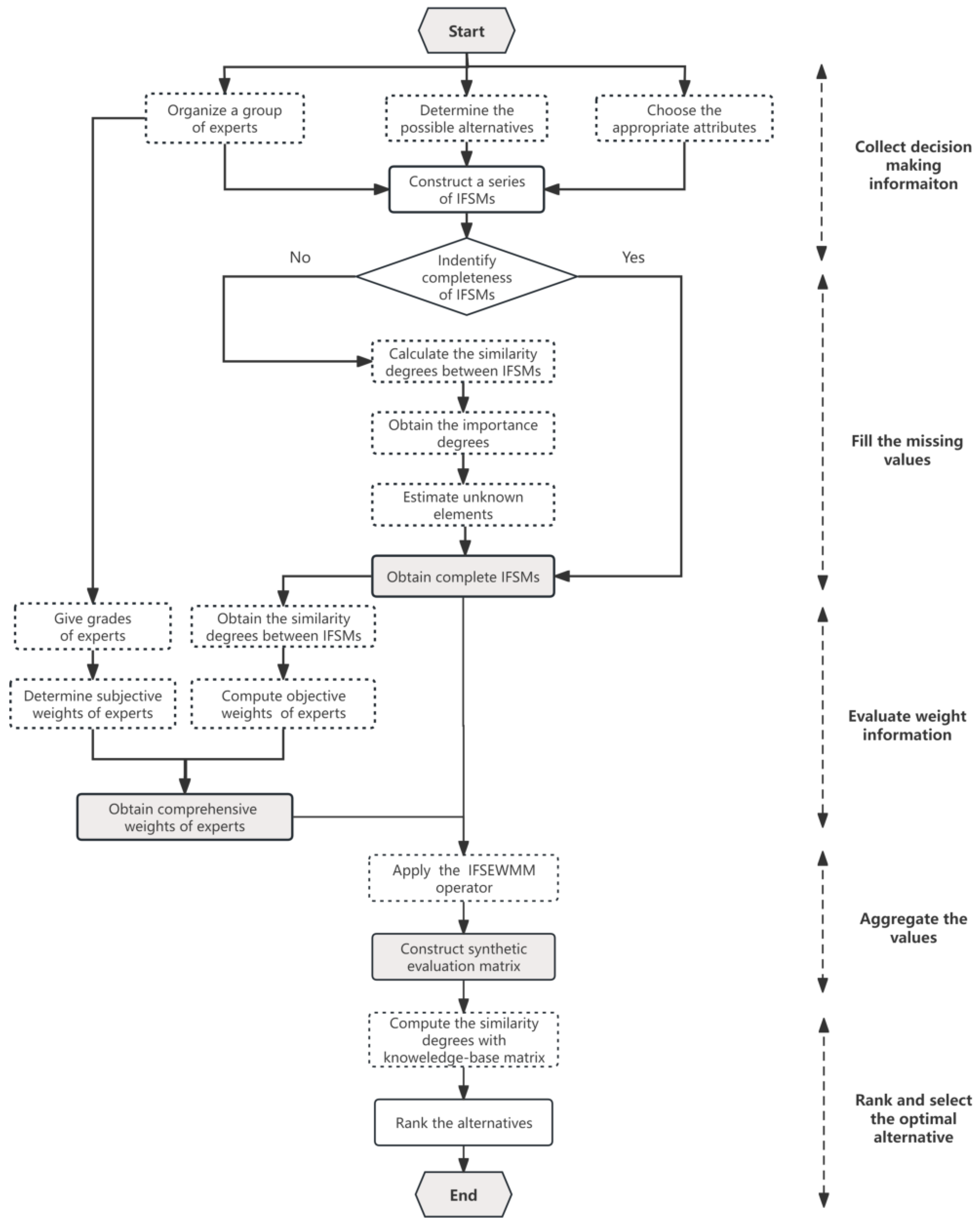
4. Group Medical Diagnosis Model with Incomplete Intuitionistic Fuzzy Soft Information

In a group medical diagnosis problem, m possible alternatives $\{x_1,x_2,\cdots ,x_m\}$ with respect to n parameters of symptoms $\{e_1,e_2,\cdots ,e_n\}$ are evaluated by q doctors $\{D_1,D_2,\cdots ,D_q\}$. Suppose that the weight ${\lambda }_k$ of doctor $D_k$ is completely unknown. The evaluation value ${\psi }_{ij}^k=({\xi }_{ij}^k,{\eta }_{ij}^k)$ of $x_i$ with respect to $e_j$ is an IFSN given by the doctor $D_k$. These values can be constructed as a series of IFSMs ${\tilde{F}}^k={\left({\psi }_{ij}^k\right)}_{m\times n}$. After fruitful discussions among the corresponding medical experts, a medical knowledge-base is expressed in terms of $\overline{F}={\left({\overline{\psi }}_{ij}^k\right)}_{m\times n}$, which consists of a set of diseases and the related set of symptoms concerned with a specific disease.

In real life, doctors have different abilities, experiences, and levels; therefore, they are always classified into different grades. Without a loss of generality, we assume that doctors can be divided into nine grades; see

Table 2. Grades of doctors.

Level	Years of Obtaining the Level	Grade
Intern	/	1
Resident doctor	$<5$	2
Resident doctor	$\ge 5$	3
Attending doctor	$<5$	4
Attending doctor	$\ge 5$	5
Associate chief physician	$<5$	6
Associate chief physician	$\ge 5$	7
Chief physician	$<5$	8
Chief physician	$\ge 5$	9

for details. Moreover, owing to the complexity of medical diagnosis problems, doctors sometimes provide incomplete evaluation values. Subsequently, we address the medical diagnosis problems step by step, which is depicted in Figure 1.

4.1. Estimation of the Missing Values of Intuitionistic Fuzzy Soft Matrices

Let ${\tilde{F}}^k={\left({\psi }_{ij}^k\right)}_{m\times n}$ be an IFSM with incomplete information. The elements ${\psi }_{ij}^k$$(i=1,2,\cdots ,m.j=1,2,\cdots ,n)$ in ${\tilde{F}}^k$ can be divided into two categories: known and missing. They are denoted, respectively, as follows:

$${ }^{+}{F}^k=\left\{{(}^{+}{\xi }_{ij}^k{,}^{+}{\eta }_{ij}^k)\right|{\xi }_{ij}^k\mathrm{and}{\eta }_{ij}^k\mathrm{are}\mathrm{known}\},$$

$${ }^{*}{F}^k=\left\{{(}^{*}{\xi }_{ij}^k,{ }^{*}{\eta }_{ij}^k)\right|{\xi }_{ij}^k\mathrm{and}{\eta }_{ij}^k\mathrm{are}\mathrm{missing}\}.$$

Obviously, ${ }^{+}{F}^k\cap { }^{*}{F}^k=\varnothing$.

Let $M^k=\left\{(i,j)\right|{(}^{*}{\xi }_{ij}^k,{ }^{*}{\eta }_{ij}^k)\in { }^{*}{F}^k\}$. $A_{ij}^k=\left\{{\tilde{F}}^l\right|{(}^{*}{\xi }_{ij}^k,{ }^{*}{\eta }_{ij}^k)\in { }^{*}{F}^k,{(}^{+}{\xi }_{ij}^l{,}^{+}{\eta }_{ij}^l)\in { }^{+}{F}^l\}$ denotes the set of IFSMs that help estimate the missing value ${\psi }_{ij}^k={(}^{*}{\xi }_{ij}^k,{ }^{*}{\eta }_{ij}^k)$.

Step 1: Calculate the degree of similarity between ${\tilde{F}}^k$ and the other matrices ${\tilde{F}}^l(l\ne k)$,

$$S{I}^{*}({\tilde{F}}^k,{\tilde{F}}^l)=\frac{1}{n-n^{kl}}\sum _{j=1}^n\left(\frac{{\displaystyle \sum _{\genfrac{}{}{0pt}{}{i=1}{(i,j)\notin M^k\cup M^l}}^m}(1-min\{|{\xi }_{ij}^k-{\xi }_{ij}^l|,|{\eta }_{ij}^k-{\eta }_{ij}^l\left|\right\})}{{\displaystyle \sum _{\genfrac{}{}{0pt}{}{i=1}{(i,j)\notin M^k\cup M^l}}^m}(1-max\{|{\xi }_{ij}^k-{\xi }_{ij}^l|,|{\eta }_{ij}^k-{\eta }_{ij}^l\left|\right\})}\right),$$

(22)

where $n^{kl}=\left|\left\{j\right|(i,j)\in M^k\cup M^l,\forall i\}\right|$.

Step 2: For unknown element ${\psi }_{ij}^k$, obtain the importance degree of ${\tilde{F}}^l\in A_{ij}^k$,

$${\lambda }_{ij}^{kl}=\frac{S{I}^{*}({\tilde{F}}^k,{\tilde{F}}^l)}{{\displaystyle \sum _{{\tilde{F}}^l\in A_{ij}^k}}S{I}^{*}({\tilde{F}}^k,{\tilde{F}}^l)}.$$

(23)

Step 3: Estimate unknown element ${\psi }_{ij}^k={(}^{*}{\xi }_{ij}^k{,}^{*}{\eta }_{ij}^k)$.

$${ }^{*}{\xi }_{ij}^k=\sum _{l\in \left\{t\right|{\tilde{F}}^t\in A_{ij}^k\}}{\lambda }_{ij}^{kl}{ }^{+}{\xi }_{ij}^l,{ }^{*}{\eta }_{ij}^k=\sum _{l\in \left\{t\right|{\tilde{F}}^t\in A_{ij}^k\}}{\lambda }_{ij}^{kl}{ }^{+}{\eta }_{ij}^l,({ }^{+}{\xi }_{ij}^l,{ }^{+}{\eta }_{ij}^l)\in { }^{+}{F}^l.$$

(24)

According to the method above, all missing values can be determined, and the IFSMs are complete.

4.2. Evaluation of Weight Information

Based on the merits and demerits of the subjective and objective information, we use the similarity measure of complete IFSMs and doctors’ grades to obtain the objective and subjective weights, respectively. Subsequently, both weights are organically combined as the comprehensive weights of doctors to overcome the shortcomings of the single-weight method to a certain extent.

Suppose that ${\lambda }^1={({\lambda }_1^1,{\lambda }_2^1,\cdots ,{\lambda }_q^1)}^T$ and ${\lambda }^2={({\lambda }_1^2,{\lambda }_2^2,\cdots ,{\lambda }_q^2)}^T$ are the subjective and objective weight vectors of the doctors, respectively. They are both completely unknown; ${\lambda }_k^1,{\lambda }_k^2\ge 0$, and ${\displaystyle \sum _{k=1}^q}{\lambda }_k^1=1,{\displaystyle \sum _{k=1}^q}{\lambda }_k^2=1$.

After obtaining the complete IFSMs using the method described in Section 4.1, the methodology for determining the comprehensive weights of the doctors includes the following steps:

Step 1: Calculate the subjective weight ${\lambda }_1^k$ of doctor $D_k$.

1.1: Use doctors’ grades to construct the preference relationship of q doctors according to the information in Table 2.

$$H={\left(d_{kt}\right)}_{q\times q}={\left(\frac{g_k}{g_t}\right)}_{q\times q},$$

(25)

where $g_k$ is the grade of doctor $D_k$.

1.2: Determine subjective weight ${\lambda }_1^k$ of the doctor $D_k$ by the analytic hierarchy process (AHP) [67].

Step 2: Utilize Equation (2) to obtain the similarity degrees between ${\tilde{F}}^k$ given by doctor $D_k$ and the other doctor’s evaluation ${\tilde{F}}^l(l\ne k)$.

$$S{I}_k=\sum _{t=1,t\ne k}^{q}SI(\widetilde{F^k},\widetilde{F^t}).$$

(26)

Step 3: Compute the objective weight ${\lambda }_2^k$ of doctor $D_k$ using the following formula,

$${\lambda }_2^k=\frac{S{I}_k}{{\displaystyle \sum _{k=1}^q}S{I}_k}.$$

(27)

Step 4: Obtain the comprehensive weight of the doctor $D_k$.

$${\lambda }^k=\alpha {\lambda }_1^k+(1-\alpha ){\lambda }_2^k,\alpha \in [0,1].$$

(28)

The appropriate parameter $\alpha$ can be chosen to describe people’s preferences for the objective and subjective weights. In the doctors’ final weights, the proportion and role of ${\lambda }_1$ and ${\lambda }_2$ will vary with the change of the parameter $\alpha$ in Equation (28). Different values of $\alpha$ may make the weights of the doctors more elastic and produce distinct results.

4.3. Approach to Group Medical Diagnosis Problem

In this subsection, we construct a model to solve group medical diagnosis problems with incomplete IFSMs, described as follows:

Step 1: Collect relevant information regarding the group medical diagnosis problems, including sets of X and E. Simultaneously, select suitable doctors and determine their grades. Later, obtain IFSM ${\tilde{F}}^{\left(k\right)}={\left({\psi }_{ij}^k\right)}_{m\times n}$ of the doctor $D_k,k\in \{1,2,\cdots ,q\}$.

Step 2: Fill in the missing values in the IFSMs (see Section 4.1 for more details). Thus, all IFSMs have complete information.

Step 3: According to the method in Section 4.2, the weight vector $\lambda ={({\lambda }_1,{\lambda }_2,\cdots ,{\lambda }_q)}^T$ is determined. Based on the unity of the subjective and objective weights, the comprehensive weights consider both people’s subjective preferences for doctors and objective differences between pieces of evaluation information. This will produce a more reliable medical diagnosis.

Step 4: Adopt the IFSEWMM operator $m\times n$ times to aggregate the values ${\psi }_{ij}^k(k=1,2,\cdots ,q)$. Construct the synthetic evaluation matrix ${\tilde{F}}^{\#}={\left({\psi }_{ij}\right)}_{m\times n}$, where ${\psi }_{ij}$ is the synthetic evaluation value of $x_i$ with respect to $e_j$:

$${\psi }_{ij}={\mathrm{IFSEWMM}}^P({\psi }_{ij}^1,{\psi }_{ij}^2,\cdots ,{\psi }_{ij}^q),(i=1,2,\cdots ,m;j=1,2,\cdots ,n).$$

(29)

Step 5: Compute the similarity degrees between $\tilde{F}\left(x_i\right)$ and $\overline{F}\left(x_i\right)$ according to Equation (2).

$$SI(\tilde{F},\overline{F})=\frac{1}{n}\sum _{j=1}^n\left(\frac{{\displaystyle \sum _{i=1}^m}(1-min\{|{\xi }_{ij}-{\overline{\xi }}_{ij}|,|{\eta }_{ij}-{\overline{\eta }}_{ij}\left|\right\})}{{\displaystyle \sum _{i=1}^m}(1-max\{|{\xi }_{ij}-{\overline{\xi }}_{ij}|,|{\eta }_{ij}-{\overline{\eta }}_{ij}\left|\right\})}\right)$$

(30)

where ${\psi }_{ij}=({\xi }_{ij},{\eta }_{ij}),{\overline{\psi }}_{ij}=({\overline{\xi }}_{ij},{\overline{\eta }}_{ij}).$

Step 6: Based on the final ranking index, select the optimal result. The larger $SI\left(x_i\right)$ is, the greater the disease $x_i$ is.

5. Numerical Example

We select a group medical diagnosis problem from [36] to illustrate the feasibility and practicality of the proposed model. Four doctors $\{D_1,D_2,D_3,D_4\}$ are grouped to determine the possible medical diagnosis of the patient. As presented in Table 2, the grades of these four doctors are $7,6,8,9$, respectively. The five possible diseases are $x_1=\mathrm{viral}\mathrm{fever}$, $x_2=\mathrm{malaria}$, $x_3=\mathrm{typhoid}$, $x_4=\mathrm{gastric}\mathrm{ulcer}$, and $x_5=\mathrm{pneumonia}$. The set of symptom parameters is $E=\{\mathrm{temperature},\mathrm{headache},\mathrm{stomach}\mathrm{pain},\mathrm{cough},\mathrm{chest}\mathrm{pain}\}$.

Table 3. Medical knowledge-base table.

	Temperature	Headache	Stomach Pain	Cough	Chest Pain
Viral fever	$(0.6,0.3)$	$(0.6,0.1)$	$(0.4,0.5)$	$(0.2,0.7)$	$(0.3,0.5)$
Malaria	$(0.7,0.1)$	$(0.3,0.6)$	$(0.1,0.6)$	$(0.5,0.4)$	$(0.1,0.8)$
Typhoid	$(0.4,0.1)$	$(0.3,0.1)$	$(0.2,0.4)$	$(0.4,0.3)$	$(0.1,0.5)$
Gastric ulcer	$(0.1,0.7)$	$(0.2,0.4)$	$(0.6,0.2)$	$(0.2,0.7)$	$(0.2,0.7)$
Pneumonia	$(0.1,0.8)$	$(0.2,0.5)$	$(0.3,0.5)$	$(0.4,0.5)$	$(0.6,0.1)$

presents the medical knowledge-base. The four doctors provide their evaluation information by means of the IFSNs shown in

Table 4. Evaluation values of doctor $D_1$.

	Temperature	Headache	Stomach Pain	Cough	Chest Pain
Viral fever	(0.3, 0.1)	(0.4, 0.1)	(0.3, 0.6)	(0.3, 0.1)	${(}^{*}{\xi }_{15}^1,{ }^{*}{\eta }_{15}^1)$
Malaria	(0.4, 0.5)	(0.1, 0.7)	(0.6, 0.2)	(0.4, 0.5)	(0.1, 0.8)
Typhoid	(0.6, 0.3)	(0.4, 0.3)	(0.5, 0.3)	(0.6, 0.2)	(0.1, 0.5)
Gastric ulcer	(0.4, 0.1)	(0.5, 0.2)	(0.5, 0.1)	(0.7, 0.2)	(0.2, 0.7)
Pneumonia	${(}^{*}{\xi }_{51}^1,{ }^{*}{\eta }_{51}^1)$	(0.2, 0.3)	(0.5, 0.3)	(0.8, 0.1)	(0.6, 0.1)

,

Table 5. Evaluation values of doctor $D_2$.

	Temperature	Headache	Stomach Pain	Cough	Chest Pain
Viral fever	(0.4, 0.2)	(0.6, 0.1)	(0.3, 0.2)	(0.2, 0.7)	(0.8, 0.1)
Malaria	(0.3, 0.5)	${(}^{*}{\xi }_{22}^2,{ }^{*}{\eta }_{22}^2)$	(0.3, 0.5)	(0.5, 0.4)	(0.4, 0.5)
Typhoid	(0.5, 0.3)	(0.5, 0.3)	(0.2, 0.4)	${(}^{*}{\xi }_{34}^2,{ }^{*}{\eta }_{34}^2)$	(0.6, 0.4)
Gastric ulcer	(0.6, 0.2)	(0.4, 0.2)	(0.6, 0.3)	(0.2, 0.7)	(0.6, 0.2)
Pneumonia	(0.4, 0.5)	(0.2, 0.5)	(0.4, 0.3)	(0.4, 0.5)	(0.4, 0.3)

,

Table 6. Evaluation values of doctor $D_3$.

	Temperature	Headache	Stomach Pain	Cough	Chest Pain
Viral fever	${(}^{*}{\xi }_{11}^3,{ }^{*}{\eta }_{11}^3)$	(0.6, 0.1)	(0.1, 0.9)	(0.3, 0.6)	(0.2, 0.4)
Malaria	(0.1, 0.7)	(0.9, 0.1)	(0.1, 0.6)	(0.4, 0.5)	(0.8, 0.1)
Typhoid	(0.5, 0.2)	(0.6, 0.3)	(0.2, 0.4)	(0.7, 0.1)	(0.9, 0.1)
Gastric ulcer	(0.6, 0.2)	(0.4, 0.5)	(0.6, 0.2)	(0.6, 0.2)	(0.3, 0.2)
Pneumonia	(0.7, 0.2)	(0.3, 0.4)	${(}^{*}{\xi }_{53}^3,{ }^{*}{\eta }_{53}^3)$	(0.5, 0.2)	(0.5, 0.4)

and

Table 7. Evaluation values of doctor $D_4$.

	Temperature	Headache	Stomach Pain	Cough	Chest Pain
Viral fever	(0.5, 0.1)	(0.2, 0.4)	(0.4, 0.6)	(0.9, 0.1)	(0.2, 0.4)
Malaria	(0.3, 0.5)	(0.5, 0.1)	(0.3, 0.5)	(0.4, 0.5)	(0.8, 0.1)
Typhoid	(0.6, 0.2)	(0.5, 0.3)	(0.2, 0.5)	(0.7, 0.1)	(0.9, 0.1)
Gastric ulcer	(0.6, 0.3)	(0.4, 0.3)	(0.4, 0.6)	(0.6, 0.2)	(0.3, 0.2)
Pneumonia	(0.4, 0.2)	(0.3, 0.5)	(0.8, 0.2)	(0.5, 0.2)	(0.5, 0.4)

, respectively. $({ }^{*}{\xi }_{ij}^k,{ }^{*}{\eta }_{ij}^k)$ denotes the corresponding missing values of $x_i$ under parameter $e_j$ given by the doctor $D_k$. Suppose that the doctors’ final weight vector $\lambda ={({\lambda }_1,{\lambda }_2,\cdots ,{\lambda }_q)}^T$ is completely unknown, where ${\lambda }_k\ge 0$ and ${\displaystyle \sum _{k=1}^q}{\lambda }_k=1$.

5.1. The Group Medical Diagnosis Process

According to the method presented in Section 4, the group medical diagnosis steps for the most likely disease the patient suffers from are described as follows:

Step 1. Estimate the missing values in the IFSMs.

1.1 Using Equation (22), the similarity measures between $F^k$ and $F^l$ $(k\ne l)$ are obtained (See details in

Table 8. Similarity measures between $F^k$ and $F^l$$(k\ne l)$.

	${\mathit{F}}_1$	${\mathit{F}}_2$	${\mathit{F}}_3$	${\mathit{F}}_4$
$F_1$	/	$0.6983$	$0.6405$	$0.6739$
$F_2$	$0.6983$	/	$0.7219$	$0.6971$
$F_3$	$0.6405$	$0.7219$	/	$0.8100$
$F_4$	$0.6739$	$0.6971$	$0.8100$	/

).

1.2 Obtain the weights of $F^l$ to aid $F^k$ by using Equation (23). See details in

Table 9. Weights of $F^l$ to aid $F^k$.

	${\mathit{F}}_1$	${\mathit{F}}_2$	${\mathit{F}}_3$	${\mathit{F}}_4$
$F_1$	/	$0.3469$	$0.3182$	$0.3348$
$F_2$	$0.3298$	/	$0.3410$	$0.3292$
$F_3$	$0.2948$	$0.3323$	/	$0.3729$

.

1.3 By using Equation (24), the filled values of intuitionistic fuzzy information are as follows:

$${(}^{*}{\xi }_{15}^1{,}^{*}{\eta }_{15}^1)=(0.4082,0.2959),{(}^{*}{\xi }_{51}^1{,}^{*}{\eta }_{51}^1)=(0.4955,0.3041),{(}^{*}{\xi }_{22}^2{,}^{*}{\eta }_{22}^2)=(0.5062,0.3099),$$

$${(}^{*}{\xi }_{34}^2{,}^{*}{\eta }_{34}^2)=(0.6773,0.1364),{(}^{*}{\xi }_{11}^3{,}^{*}{\eta }_{11}^3)=(0.4078,0.1332),{(}^{*}{\xi }_{53}^3{,}^{*}{\eta }_{53}^3)=(0.5786,0.2627).$$

Step 2. Determine the weight vector of the doctors.

2.1 The preference matrix according to the grades of the doctors is

$$H=\left(\begin{array}{cccc}1& \frac{7}{6}& \frac{7}{8}& \frac{7}{9}\\ \frac{6}{7}& 1& \frac{6}{8}& \frac{6}{9}\\ \frac{8}{7}& \frac{8}{6}& 1& \frac{8}{9}\\ \frac{9}{7}& \frac{9}{6}& \frac{9}{8}& 1\end{array}\right).$$

By the analytic hierarchy process (AHP), the subjective weight vector of the doctors is obtained as

$${\lambda }_1={(0.2333,0.2,0.2667,0.3)}^T.$$

2.2 Utilize Equation (2) to calculate the similarity measures between IFMSs with the complete information obtained in Step 1. See details in

Table 10. Similarity measures between $F^k$ and $F^l$.

	${\mathit{F}}_1$	${\mathit{F}}_2$	${\mathit{F}}_3$	${\mathit{F}}_4$
$F_1$	/	$0.6869$	$0.6666$	$0.6838$
$F_2$	$0.6869$	/	$0.7268$	$0.7117$
$F_3$	$0.6666$	$0.7268$	/	$0.8164$
$F_4$	$0.6838$	$0.7117$	$0.8164$	/

.

By using Equation (27), the objective weight vector of the doctors is obtained as

$${\lambda }_2={(0.2373,0.2476,0.2574,0.2577)}^T.$$

2.3 $\alpha =0.5$, so the weight vector of the doctors is $\lambda ={(0.2353,0.2238,0.2621,0.2788)}^T.$

Step 3. Let $P=(1,1,1,1)$. Using Equation (29), obtain the collective evaluation value ${\psi }_{ij}$ of $x_i$ with respect to the $e_j$ in

Table 11. Collective evaluation values.

	Temperature	Headache	Stomach Pain	Cough	Chest Pain
Viral fever	(0.4029, 0.0983)	(0.4318, 0.1248)	(0.2592, 0.3681)	(0.3603, 0.2669)	(0.3663, 0.2185)
Malaria	(0.2613, 0.3605)	(0.4144, 0.2295)	(0.2917, 0.3127)	(0.4316, 0.3267)	(0.4174, 0.2704)
Typhoid	(0.5419, 0.1889)	(0.4968, 0.2238)	(0.2696, 0.2871)	(0.6456, 0.0993)	(0.4875, 0.2060)
Gastric ulcer	(0.5380, 0.1467)	(0.4316, 0.2234)	(0.5220, 0.2228)	(0.4840, 0.2467)	(0.3407, 0.2470)
Pneumonia	(0.4922, 0.2259)	(0.2587, 0.3007)	(0.5396, 0.2002)	(0.5362, 0.1880)	(0.4972, 0.2199)

.

Step 4. Compute the similarity degrees $SI\left(x_i\right)$ between $\tilde{F}\left(x_i\right)$ and $\overline{F}\left(x_i\right)(i=1,2,3,4,5)$, which yields the following:

$$SI\left(x_1\right)=0.7896,SI\left(x_2\right)=0.6965,SI\left(x_3\right)=0.7910,SI\left(x_4\right)=0.6682,SI\left(x_5\right)=0.7146.$$

Step 5. Based on the ranking index for each disease, the diseases are ranked as $x_3\succ x_1\succ x_5\succ x_2\succ x_4$. Obviously, typhoid is most likely the disease that the patient suffers from.

5.2. Discussion

5.2.1. Comparative Analysis

To illustrate the superiority of the proposed group medical diagnosis model further, we use the methods described in Refs. [7,8,36,55,62] to solve the medical diagnosis problem above.

Table 12. Diagnosis results obtained by different methods.

Method	Parameter Values	Ranking Order	Diagnosis Result
Mao (2013) [8]	/	$x_1\succ x_3\succ x_5\succ x_2\succ x_4$	Viral fever
Das (2014) [7]	/	$x_3\succ x_1\succ x_5\succ x_2\succ x_4$	Typhoid
Hu (2019) [36]	$p=1,q=1$	$x_3\succ x_1\succ x_5\succ x_4\succ x_2$	Typhoid
Arora (2020) [55]	/	$x_3\succ x_1\succ x_5\succ x_4\succ x_2$	Typhoid
Chen (2020) [62]	/	$x_3\succ x_1\succ x_5\succ x_4\succ x_2$	Typhoid
	$P=(1,0,0,0)$	$x_3\succ x_1\succ x_5\succ x_4\succ x_2$	Typhoid
The proposed	$P=(1,1,0,0)$	$x_3\succ x_1\succ x_5\succ x_4\succ x_2$	Typhoid
method	$P=(1,1,1,0)$	$x_1\succ x_3\succ x_5\succ x_2\succ x_4$	Viral fever
	$P=(1,1,1,1)$	$x_3\succ x_1\succ x_5\succ x_2\succ x_4$	Typhoid

shows the diagnosis results obtained using the different methods. It has been documented that the results obtained by the proposed method are comparable to those obtained by the predominating methods. This indicates that the proposed model is valid and feasible.

As presented in Table 12, the diagnosis results of the six methods are slightly different. Comparative analyses of the proposed method with the prevailing approaches are elaborated as follows:

(1)

The intuitionstic fuzzy soft weighted Einstein averaging operator is based on Einstein operations [55], which is the same as the IFSEWMM operator. The intuitionstic fuzzy soft weighted Einstein averaging operator can fuse fuzzy information easily. However, it considers that the aggregated arguments are independent. The IFSEWMM operator captures the interrelationships among the input arguments, whereas the intuitionstic fuzzy soft weighted Einstein averaging operator does not possess this property. By taking the parameter $P=(1,0,\cdots ,0)$, the IFSEWMM operator reduces to the intuitionstic fuzzy soft weighted Einstein averaging operator. Hence, the IFSEWMM operator can handle both cases, that is, whether the input arguments are dependent or independent. Therefore, the IFSEWMM operator is more general and flexible than the intuitionstic fuzzy soft weighted Einstein averaging operator in [55];

(2)

The weighted intuitionstic fuzzy soft Bonferroni mean operator was constructed based on the BM operator [36]. It considers only the relationships between any two input arguments [36]. In actual decision-making problems, the interrelationship among more than two input arguments must be considered. The weighted intuitionstic fuzzy soft Bonferroni mean operator cannot solve this problem. Similar to the MM operator, the presence of parameter P makes the IFSEWMM operator consider the interconnection among two or more arguments. Compared to the weighted intuitionstic fuzzy soft Bonferroni mean operator, the IFSEWMM operator is more flexible;

(3)

In [62], missing values of ${\tilde{F}}^k$ were estimated according to the average of known values in other IFSMs ${\tilde{F}}^l(k\ne l)$. Owing to the relationship between doctors, the IFSMs given by different doctors work differently. Therefore, we cannot ignore the degree of importance of other IFSMs. Evidently, the higher the degree of similarity between IFSM ${\tilde{F}}^k$ and IFSM ${\tilde{F}}^l$ is, the closer the values are. Thus, the higher the degree of similarity between ${\tilde{F}}^k$ and ${\tilde{F}}^l$, the greater the weight of the doctor $D_l$ that should be assigned in the estimation of unknown values process. In this study, we use the similarity degrees between ${\tilde{F}}^k$ and the other matrices ${\tilde{F}}^l(l\ne k)$ to determine the importance degree of ${\tilde{F}}^l$ for ${\tilde{F}}^l$. Those estimated values are closer to reality.

5.2.2. Sensitivity Analysis

This subsection analyzes the influences of parameter vector P on the IFSEWMM operator and $\alpha$ in Equation (28) for the diagnosis results.

To recognize the impact of parameter vector P during group medical diagnosis, an analysis is conducted to choose different values of P. Let the weight vector of doctors be $\lambda ={(0.2353,0.2238,0.2621,0.2788)}^T$. The realization of the IFSEWMM operator is performed according to the parameter vector P. Figure 2 provides an intuitive sense of the influence of the parameter P on the medical diagnosis results. When P is $(1,1,1,0)$, the patient is most likely to suffer from viral fever. All the other cases are typhoid. When $P=(1,0,0,0),(2,0,0,0)$, or $(3,0,0,0)$, the interrelationships among the attributes are not considered. The vectors $P=(1,1,0,0)$ and $P=(1,1,1,0)$ capture the interrelationship between any two or three attributes. However, $P=(1,1,1,1)$ and $P=(0.25,0.25,0.25,0.25)$ both recognize the interrelationships among all objects.

Let $P=(1,1,1,1)$. The medical diagnosis results with different $\alpha$ values in Equation (28) are illustrated in Figure 3. As shown in Figure 3, the ordering of alternatives is slightly different, with a varying value of $\alpha$, which confers people’s preferences. Thus, when a different $\alpha$ is chosen, the decision-making results will be changed accordingly. This can provide more flexible and reasonable choices for doctors. Therefore, the significance of $\alpha$ must be precisely considered in group medical diagnosis problems. This also shows that doctors’ weights affect the diagnosis results. Additionally, the weights of doctors are determined either by a completely subjective method or by the established norms in Refs. [7,8,55,62]. As in [36], we obtain the comprehensive weight information for each doctor by considering both subjective and objective weights. The objective weights are calculated based on similarity measures between IFSMs. Conversely, according to the doctor’ grades, a comparison matrix is constructed to obtain subjective weights. The comprehensive weights of doctors are obtained using a linear combination, and are more reasonable and comprehensive than the results obtained by a single method.

Based on the comparison and sensitivity analysis, the advantages of the proposed approach for group medical diagnosis problems with incomplete intuitionistic fuzzy soft information are summarized as follows:

(a)

Different parameter vectors may produce different ranking results because parameter vector P represents the risk preferences of people. Additionally, many operators become special cases of the proposed operators under some suitable conditions (when P or $\lambda$ is assigned a specific number). Novel operators are more generalized and flexible in handling different GDM problems;

(b)

Weight information about experts obtained by combining subjective and objective weights can reflect people’s preferences while reducing the randomness of the results;

(c)

Considering the different influences of other IFSMs, the estimated values in an incomplete IFSM are more in line with the actual situation.

In summary, the proposed method is more comprehensive, and can provide more flexible and reasonable choices for GDM models.

6. Conclusions

This study combines the MM operator with Einstein operations to develop two novel intuitionistic fuzzy soft weighted Muirhead mean operators. These two novel operators are bounded and monotonic with respect to the input arguments but not idempotent. Furthermore, a group decision-making model with incomplete intuitionistic fuzzy soft information for medical diagnosis is constructed. The similarity measures of IFSMs given by experts fill in the missing values in a mathematical manner that differs from previous works. Subsequently, the grades of the doctors and similarity degrees of the IFSMs are utilized to obtain the subjective and objective weights, respectively. Simultaneously, the combined weights, which can overcome the shortcomings of the single-weight method to some extent, are determined. Finally, the GDM model is implemented to investigate its applicability to a group medical diagnosis problem. Through comparison and analysis of the practical diagnosis process, the proposed model is demonstrated as being effective.

The following are limitations and future research directions: (1) Unlike the basic algebraic sum and product operations, the calculations for the Einstein sum and product are more complicated. Therefore, when the newly constructed intuitionistic fuzzy soft operators based on Einstein operations are used to aggregate information, the number of calculations increases. The question of how to use a simple and appropriate method to solve GDM problems quickly and effectively requires further study; (2) The proposed model will be adjusted or improved for application to other extensions of fuzzy sets, and different decision problems will be handled according to different application backgrounds; (3) Using relevant data from the machine learning repository dataset, medical diagnoses will be simulated to further validate the rationality of the algorithm and optimize the model. We will consult doctors and use clinical data to determine the main diagnostic features and medical knowledge-base of different diseases. It can be used to provide basic diagnostic consulting services.

References

1. Nan, T.B.; Zhang, H.; He, Y. Pythagorean fuzzy full implication triple i method and its application in medical diagnosis. Int. J. Fuzzy Syst. 2022, 24, 2250–2263. [Google Scholar] [CrossRef]
2. Ding, J.J.; Li, D.Y.; Zhang, C.; Lin, M.W. Three-way group decisions with evidential reasoning in incomplete hesitant fuzzy information systems for liver disease diagnosis. Appl. Intell. 2023, 53, 29693–29712. [Google Scholar] [CrossRef]
3. Pham, H.V.; Hoang, T.L.; Hung, N.Q.; Phung, T.K. Proposed intelligent decision support system using hedge algebra integrated with picture fuzzy relations for improvement of decision-making in medical diagnoses. Int. J. Fuzzy Syst. 2023, 25, 3260–3270. [Google Scholar] [CrossRef]
4. Shao, Z.; Kosari, S.; Rashmanlou, H.; Mofidnakhaei, F. Fuzzy decision making in medical diagnosis using vague sets. J. Mult.-Valued Log. Soft Comput. 2023, 40, 137–153. [Google Scholar]
5. Liu, M.; Zhang, X.; Mo, Z. A modified correlation coefficient of probabilistic hesitant fuzzy sets and its applications of decision making, medical diagnosis, cluster analysis. Int. J. Fuzzy Syst. 2023, 25, 2609–2627. [Google Scholar] [CrossRef]
6. Ye, J.; Sun, B.Z.; Bai, J.C.; Bao, Q.; Chu, X.L.; Bao, K. A preference-approval structure-based non-additive three-way group consensus decision-making approach for medical diagnosis. Inform. Fusion 2024, 101, 102008. [Google Scholar] [CrossRef]
7. Das, S.; Kar, S. Group decision making in medical system: An intuitionistic fuzzy soft set approach. Appl. Soft Comput. 2014, 24, 196–211. [Google Scholar] [CrossRef]
8. Mao, J.; Yao, D.; Wang, C. Group decision making methods based on intuitionistic fuzzy soft matrices. Appl. Math. Model. 2013, 37, 6425–6436. [Google Scholar] [CrossRef]
9. Hussain, A.; Zhu, X.Y.; Ullah, K.; Sarfaraz, M.; Yin, S.; Pamucar, D. Multi-attribute group decision-making based on Pythagorean fuzzy rough Aczel-Alsina aggregation operators and its applications to Medical diagnosis. Heliyon 2023, 9, e23067. [Google Scholar] [CrossRef]
10. Hwang, C.L.; Lin, M.J. Group Decision Making under Multiple Criteria: Methods and Applications; Springer Science & Business Media: Berlin/Heidelberg, Germany, 2012. [Google Scholar]
11. Adlassnig, K.P. Fuzzy set theory in medical diagnosis. IEEE Trans. Syst. Man Cybern. 1986, 16, 260–265. [Google Scholar] [CrossRef]
12. Zadeh, L.A. Fuzzy sets. Inf. Control 1965, 8, 338–353. [Google Scholar] [CrossRef]
13. Atanassov, K.T. Intuitionistic fuzzy set. Fuzzy Sets Syst. 1986, 20, 87–96. [Google Scholar] [CrossRef]
14. Li, Z.W.; Wen, G.; Xie, N. An Approach to Fuzzy Soft Sets in Decision Making Based on Grey Relational Analysis and Dempster-Shafer Theory of Evidence: An Application in Medical Diagnosis; Elsevier Science Publishers Ltd.: Amsterdam, The Netherlands, 2015. [Google Scholar]
15. Wang, J.; Hu, Y.; Xiao, F.; Deng, X.; Deng, Y. A novel method to use fuzzy soft sets in decision making based on ambiguity measure and dempster-shafer theory of evidence: An application in medical diagnosis. Artif. Intell. Med. 2016, 69, 1–11. [Google Scholar] [CrossRef] [PubMed]
16. Xiao, F.Y. A hybrid fuzzy soft sets decision making method in medical diagnosis. IEEE Access 2018, 6, 25300–25312. [Google Scholar] [CrossRef]
17. Thao, N.X.; Ali, M.; Nhung, L.T.; Gianey, H.K.; Smarandache, F. A new multi-criteria decision making algorithm for medical diagnosis and classification problems using divergence measure of picture fuzzy sets. J. Intell. Fuzzy Syst. 2019, 37, 7785–7796. [Google Scholar] [CrossRef]
18. Guleria, A.B.R.K. On pythagorean fuzzy soft matrices, operations and their applications in decision making and medical diagnosis. Soft Comput. 2019, 23, 7889–7900. [Google Scholar] [CrossRef]
19. Zhang, R.C.; Gou, X.; Xu, Z. A multi-attribute decision-making framework for Chinese medicine medical diagnosis with correlation measures under double hierarchy hesitant fuzzy linguistic environment. Comput. Ind. Eng. 2021, 156, 107243. [Google Scholar] [CrossRef]
20. Sangodapo, T.O.; Onasanya, B.O.; Mayerova-Hoskova, S. Decision-making with fuzzy soft matrix using a revised method: A case of medical diagnosis of diseases. Mathematics 2021, 9, 2327. [Google Scholar] [CrossRef]
21. Farhadinia, B. A divergence-based medical decision-making process of COVID-19 diagnosis. Math. Probl. Eng. 2022, 2022, 7685033. [Google Scholar] [CrossRef]
22. Bui, Q.T.; Ngo, M.P.; Snasel, V.; Pedrycz, W.; Vo, B. The sequence of neutrosophic soft sets and a decision-making problem in medical diagnosis. Int. J. Fuzzy Syst. 2022, 24, 2036–2053. [Google Scholar] [CrossRef]
23. Molodtsov, D. Soft set theory—First results. Comput. Math. Appl. 1999, 37, 19–31. [Google Scholar] [CrossRef]
24. Maji, P.K.; Biswas, R.; Roy, A.R. Intuitionistic fuzzy soft sets. J. Fuzzy Math. 2001, 9, 677–692. [Google Scholar]
25. Jiang, Y.; Tang, Y.; Liu, H.; Chen, Z. Entropy on intuitionistic fuzzy soft sets and on interval-valuedfuzzy soft sets. Inf. Sci. 2013, 240, 95–114. [Google Scholar] [CrossRef]
26. Khalid, A.; Abbas, M. Distance measures and operations in intuitionistic and interval-values intuitionistic fuzzy soft set theory. Int. J. Fuzzy Syst. 2015, 17, 490–497. [Google Scholar] [CrossRef]
27. Muthukumar, P.; Krishnan, G.S.S. A similarity measure of intuitionistic fuzzy soft sets and its application in medical diagnosis. Appl. Soft Comput. 2016, 41, 148–156. [Google Scholar] [CrossRef]
28. Rajarajeswari, P.; Dhanalakshmi, D.P. Similarity measures of intuitionistic fuzzy soft sets and their application in medical diagnosis. Int. J. Math. Arch. 2014, 5, 143–149. [Google Scholar]
29. Garg, H.; Arora, R. TOPSIS method based on correlation coefficient for solving decision-making problems with intuitionistic fuzzy soft set information. Aims Math. 2020, 5, 2944–2966. [Google Scholar] [CrossRef]
30. Feng, F.; Xu, Z.S.; Fujita, H.; Liang, M.Q. Enhancing PROMETHEE method with intuitionistic fuzzy soft sets. Int. J. Intell. Syst. 2020, 35, 1071–1104. [Google Scholar] [CrossRef]
31. Xie, N.X.; Li, Z.W.; Zhang, G.Q. An intuitionistic fuzzy soft set method for stochastic decision-making applying prospect theory and grey relational analysis. J. Intell. Fuzzy Syst. 2017, 33, 15–25. [Google Scholar] [CrossRef]
32. Seikh, M.R.; Mandal, U. Multiple attribute group decision making based on quasirung orthopair fuzzy sets: Application to electric vehicle charging station site selection problem. Eng. Appl. Artif. Intell. 2022, 115, 105299. [Google Scholar] [CrossRef]
33. Arora, R.; Garg, H. Prioritized averaging/geometric aggregation operators under the intuitionistic fuzzy soft set environment. Sci. Iran. 2018, 25, 466–482. [Google Scholar] [CrossRef]
34. Arora, R.; Garg, H. Robust aggregation operators for multi-criteria decision-making with intuitionistic fuzzy soft set environment. Sci. Iran. Trans. E Ind. Eng. 2018, 25, 931–942. [Google Scholar] [CrossRef]
35. Garg, H.; Arora, R. Bonferroni mean aggregation operators under intuitionistic fuzzy soft set environment and their applications to decision-making. J. Oper. Res. Soc. 2018, 69, 1711–1724. [Google Scholar] [CrossRef]
36. Hu, J.H.; Pan, L.; Yang, Y.; Chen, H.W. A group medical diagnosis model based on intuitionistic fuzzy soft sets. Appl. Soft Comput. 2019, 77, 453–466. [Google Scholar] [CrossRef]
37. Maclaurin, C. A second letter to Martin Folkes, Esq; concerning the roots of equations, with demonstration of other rules of algebra. Philos. Trans. R. Soc. A 1729, 36, 59–96. [Google Scholar]
38. Bonferroni, C. Sulle medie multiple di potenze. Boll. de Uni. Mate Ital. 1950, 5, 267–270. [Google Scholar]
39. Garg, H.; Arora, R. Generalized Maclaurin symmetric mean aggregation operators based on Archimedean t norm of the intuitionistic fuzzy soft set information. Art Intell. Rev. 2021, 54, 3173–3213. [Google Scholar] [CrossRef]
40. Muirhead, R.F. Some methods applicable to identities and inequalities of symmetric algebraic functions of n letters. Proc. Edinb. Math. Soc. 1902, 21, 144–162. [Google Scholar] [CrossRef]
41. Zhong, Y.R.; Zhang, H.N.; Cao, L.B.; Li, Y.Y.; Qin, Y.C.; Luo, X.N. Power Muirhead mean operators of interval-valued intuitionistic fuzzy values in the framework of Dempster-Shafer theory for multiple criteria decision-making. Soft Comput. 2023, 27, 763–782. [Google Scholar] [CrossRef]
42. Hong, Z.; Rong, Y.; Qin, Y. Hesitant fuzzy dual Muirhead mean operators and its application to multiple attribute decision making. J. Intell. Fuzzy Syst. 2018, 35, 2161–2172. [Google Scholar] [CrossRef]
43. Wang, J.; Zhang, R.; Zhu, X. Some hesitant fuzzy linguistic Muirhead means with their application to multiattribute group decision-making. Complexity 2018, 2018, 5087851. [Google Scholar] [CrossRef]
44. Liu, P.; Li, Y.; Zhang, M. Multiple-attribute decision-making method based on hesitant fuzzy linguistic Muirhead mean aggregation operators. Soft Comput. 2018, 2, 5513–5524. [Google Scholar] [CrossRef]
45. Zhu, J.; Li, Y. Pythagorean fuzzy Muirhead mean operators and their application in multiple-criteria group decision-Making. Information 2018, 9, 142. [Google Scholar] [CrossRef]
46. Wang, R. Research on the application of the financial investment risk appraisal models with some interval number muirhead mean operators. J. Intell. Fuzzy Syst. 2019, 19, 1064–1246. [Google Scholar] [CrossRef]
47. Mahmood, T.; Haleemzai, I.; Ali, Z.; Pamucar, D.; Marinkovic, D. Power muirhead mean operators for interval-valued linear diophantine fuzzy sets and their application in decision-making strategies. Mathematics 2022, 10, 70. [Google Scholar] [CrossRef]
48. Seikh, M.R.; Mandal, U. Intuitionistic fuzzy dombi aggregation operators and their application to multiple attribute decision-making. Granular Comput. 2021, 6, 473–488. [Google Scholar] [CrossRef]
49. Seikh, M.R.; Mandal, U. q-Rung Orthopair Fuzzy Archimedean Aggregation Operators: Application in the Site Selection for Software Operating Units. Symmetry 2023, 15, 1680. [Google Scholar] [CrossRef]
50. Du, W.S. A further investigation on q-rung orthopair fuzzyEinstein aggregation operators. J. Intell. Fuzzy Syst. 2021, 41, 6655–6673. [Google Scholar] [CrossRef]
51. Wang, W.Z.; Liu, X.W. Intuitionistic fuzzy information aggregation using Einstein operations. IEEE Trans. Fuzzy Syst. 2012, 20, 923–938. [Google Scholar] [CrossRef]
52. Garg, H. Generalized intuitionistic fuzzy interactive geometric interation operators using Einstein t-norm and t-conorm and their application to decision making. Comput. Ind. Eng. 2016, 101, 53–69. [Google Scholar] [CrossRef]
53. Khan, M.S.A.; Abdullah, S.; Ali, A. Multiattribute group decision-making based on Pythagorean fuzzy Einstein prioritized aggregation operators. Int. J. Intell. Syst. 2019, 34, 1001–1033. [Google Scholar] [CrossRef]
54. Liu, P.D.; Wang, P. Multiple attribute group decision making method based on intuitionistic fuzzy Einstein interactive operations. Int. J. Fuzzy Syst. 2020, 22, 790–809. [Google Scholar] [CrossRef]
55. Arora, R. Intuitionistic fuzzy soft aggregation operator based on einstein norms and its applications in decision-making. In Proceedings of the Intelligent Systems Design and Applications: 18th International Conference on Intelligent Systems Design and Applications (ISDA 2018), Vellore, India, 6–8 December 2018; Volume 940, pp. 998–1008. [Google Scholar]
56. Zhang, X.L.; Xu, Z.S. Soft computing based on maximizing consensus and fuzzy TOPSIS approach to interval-valued intuitionistic fuzzy group decision making. Appl. Soft Comput. 2015, 26, 42–56. [Google Scholar] [CrossRef]
57. Abootalebi, S.; Hadi-Vencheh, A.; Jamshidi, A. An improvement to determining expert weights in group multiple attribute decision making problem. Group Decis. Negot. 2018, 27, 215–221. [Google Scholar] [CrossRef]
58. Li, W.M.; Ye, J. MAGDM model using an intuitionstic fuzzy matrix energy method and its application in the selection issue of hospital locations. Axioms 2023, 12, 766. [Google Scholar] [CrossRef]
59. Das, S.; Ghosh, S.; Kar, S.; Pal, T. An algorithmic approach for predicting unknown information in incomplete fuzzy soft set. Arab. J. Sci. Eng. 2017, 42, 3563–3571. [Google Scholar] [CrossRef]
60. Zou, Y.; Xiao, Z. Data analysis approaches of soft sets under incomplete information. Knowl. Based Syst. 2008, 21, 941–945. [Google Scholar] [CrossRef]
61. Kong, Z.; Zhang, G.D.; Wang, L.F.; Wu, Z.X.; Qi, S.Q.; Wang, H.F. An efficient decision making approach in incomplete soft set. Appl. Math. Model. 2014, 38, 2141–2150. [Google Scholar] [CrossRef]
62. Chen, X.G.; Yu, G.F.; Wu, J.; Yang, Y. A minimum trust discount coefficient model for incomplete information in group decision making with intuitionistic fuzzy soft set. Int. J. Fuzzy Syst. 2020, 22, 2025–2040. [Google Scholar] [CrossRef]
63. Qin, H.; Ma, X. Data analysis approaches of interval-valued fuzzy soft sets under incomplete information. IEEE Access 2019, 7, 3561–3571. [Google Scholar] [CrossRef]
64. Qin, H.W.; Li, H.F.; Ma, X.Q.; Gong, Z.Y.; Cheng, Y.T.; Fei, Q.H. Data analysis approach for incomplete interval-valued intuitionistic fuzzy soft sets. Symmetry 2020, 12, 1061. [Google Scholar] [CrossRef]
65. Ma, X.; Han, Y.; Qin, H.; Wang, P. KNN data filling algorithm for incomplete interval-valued fuzzy soft sets. Int. J. Comput. Int. Syst. 2023, 16, 30. [Google Scholar] [CrossRef]
66. Qin, J.D.; Liu, X.W. 2-tuple linguistic Muirhead mean operators for multiple attribute group decision making and its application to supplier selection. Kybe 2016, 45, 2–29. [Google Scholar] [CrossRef]
67. Saaty, T.L. The Analytic Hierarchy Process; McGraw-Hill: New York, NY, USA, 1980. [Google Scholar]
Figure 1. General framework of the proposed model.
Mathematics 12 01823 g001
Figure 2. Diagnosis results of different parameter vector P.
Mathematics 12 01823 g002
Figure 3. Diagnosis results under different α values when P = (1,1,1,1).
Mathematics 12 01823 g003