Influence of the Effective Reproduction Number on the SIR Model with a Dynamic Transmission Rate

Abstract

In this paper, we examine the epidemiological model B-SIR, focusing on the dynamic law that governs the transmission rate $\mathbf{B}$. We define this dynamic law by the differential equation ${\mathbf{B}}^{\prime }/\mathbf{B}={\mathbf{F}}_{\oplus }-{\mathbf{F}}_{\ominus }$, where ${\mathbf{F}}_{\ominus }$ represents a reaction factor reflecting the stress proportional to the active group’s percentage variation. Conversely, ${\mathbf{F}}_{\oplus }$ is a factor proportional to the deviation of $\mathbf{B}$ from its intrinsic value. We introduce the notion of contagion impulse f and explore its role within the model. Specifically, for the case where ${\mathbf{F}}_{\oplus }=0$, we derive an autonomous differential system linking the effective reproductive number with f and subsequently analyze its dynamics. This analysis provides new insights into the model’s behavior and its implications for understanding disease transmission.

1. Introduction

At the beginning of the COVID-19 pandemic, when no vaccines were available, one of the natural concerns in almost all countries was to flatten the epidemic curve to avoid the collapse of the healthcare sector [1,2,3]. Through the ordinance and implementation of non-pharmaceutical mitigation measures recommended by experienced or specialized agencies, such as WHO, the urgent task was not to exceed the maximum healthcare capacity [4,5], thus saving the lives of critically ill patients and avoiding having to make difficult decisions about who should receive care [6,7]. However, the instances of hospital collapses increased as the pandemic progressed. This collapse was not limited to care but extended to postmortem services: forensic work, morgues, funeral services, and cemeteries [8,9,10,11].

The concern about not exceeding the capacity of the healthcare systems became prominent among modelers at the beginning of the pandemic [12,13]. It was important for models to be simple enough in technical terms to be understood and, simultaneously, to capture the structure of the relationships of the determinants and their connection with the variables of epidemiological interest. This strategic character [14], summarized in expressions such as “The simplest models can be of great benefit in predicting and monitoring epidemics, helping to understand the dynamics of the COVID-19 pandemic and contribute to decision-making” [15], or “Models should not be simpler than necessary, but also not more complex than needed”, became necessary and valued [16,17,18].

In the experience of the COVID-19 pandemic, one of the critical indicators for decision making, even in the first months of the pandemic, was the effective reproductive number, here denoted as ${\mathcal{R}}_e$, [19,20,21,22]. Among the curves to be followed for frequent follow-up by health teams, apart from new daily cases, total cases, or cumulative cases, the curve of ${\mathcal{R}}_e$ versus time is prioritized. Non-pharmaceutical mitigation efforts had, in this number, been an indicator of the disease’s state and its reflection of the effectiveness of the control exercised.

This article is inspired by work that aims to incorporate human behavior, which, for a specific population, translates into alterations in transmission rate, incorporating variability. In particular, focusing on the case in which a specific law governs the transmission rate, as is the case of the $\beta$-SEIR model introduced in [23,24], the objective of this paper is to show situations in which the command and response of the citizenry reach a certain correspondence with a control that monitors ${\mathcal{R}}_e$, more precisely, its proximity to the unitary threshold, which marks the possibility of slowing down the spread of the disease.

Although, in the case of advanced development, we are referring to when the number of susceptible people has dropped considerably, ${\mathcal{R}}_e$ naturally decreases, the critical thing is that the control of the daily number of new infections is vital to not saturating systems so that they can adequately meet the demand and not become another source of infection and ethical conflicts associated with whom and whom not to treat.

We will analyze two cases depending on the immediacy of the reaction to the ${\mathcal{R}}_e$ indicator: (a) one when the citizen response to the control is rapid and at different scales of compliance and another (b) when there is a lag or delay in the materialization of control, occurring at different levels of compliance. An important aspect to consider is that if ${\mathcal{R}}_e$ is less than one, there is room to relax the system somewhat.

2. Materials and Methods

In a previous study [23], a transmission rate $\mathbf{B}$ is proposed that is in permanent tension between a force that reacts to lower the transmission rate and another that aims to resist or restore its intrinsic value. More precisely, it takes the following form:

$${\mathbf{B}}^{\prime }/\mathbf{B}={\mathbf{F}}_{\oplus }-{\mathbf{F}}_{\ominus },$$

where the minuend and subtrahend, ${\mathbf{F}}_{\oplus }$ and ${\mathbf{F}}_{\ominus }$, are called the restitution factor and reaction factor, respectively. Thus, $\mathbf{B}$ decreases or increases as ${\mathbf{F}}_{\ominus }$ is greater or less than ${\mathbf{F}}_{\oplus }$.

Let us note that an important assumption for specific formulations of ${\mathbf{F}}_{\ominus }$ is that the health authority, to mitigate action (lowering the transmission rate), makes decisions from a measure that reflects the current risk of contagion, and this is from some of the state variables that could be followed as data. Therefore, assuming a baseline SIR-type propagation model, it is understood that the reaction factor responds to an evaluation of the $(S,I,R)$ state variable, i.e.,

$${\mathbf{F}}_{\ominus }={\mathbf{F}}_{\ominus }(S,I,R,S^{\prime },I^{\prime },R^{\prime })$$

It is a direct function of some state components or their variations and how fast they vary.

In [23], the authors study a case in which, at each instant, the mitigating reaction depends on evaluating the number of assets, i.e.,

$$\left(\mathrm{a}\right) {\mathbf{F}}_{\ominus }\left(I\right)=\mu ·I, \mathrm{with} \mu >0.$$

On the other hand, in [24], a case in which this reaction depends on the daily variation of the active group, i.e.,

$$\left(\mathrm{b}\right) {\mathbf{F}}_{\ominus }\left(I^{\prime }\right)=\mu ·I^{\prime }, \mathrm{with} \mu >0,$$

is also analyzed.

Regarding case (a), criticism arises from the observation that the number of infectious agents a few days after an epidemic begins differs significantly from that after months. In response, the paper assumes that the µ coefficient varies over time, illustrated by its association with the rigor of the moment, such as the stringency index. In case (b), the same observation can be made; it is not the same to have a variation of one thousand cases if the active group is five thousand as if the base of this variation is twenty thousand.

In this sense, the commonality between cases (a) and (b) is that they are reaction factors based on absolute numbers, like the number of infections in case (a) or their variation per unit of time (e.g., daily) for (b). A reaction that considers a relative appreciation of the situation seems more adequate to measure the moment’s impact. That is, as a measure of the magnitude of the contagion process, it is more comparable when, given five thousand active cases yesterday, we see an increase to 500 new cases, compared with having a base of ten thousand active cases and increasing to 1000 cases, representing a similar increase of 10% in both cases.

Thus, a reaction factor that is associated with a risk perception proportional to the percentage variation, for example, daily, of the active group, can be expressed as follows:

$$\left(\mathrm{c}\right) {\mathbf{F}}_{\ominus }=\mu ·\{I^{\prime }/I\}, \mathrm{with} \mu >0.$$

If we continue to assume the SIR model as the base model, we have the following:

$$I^{\prime }/I=\beta (S/N)-\gamma =\gamma \left({\mathcal{R}}_e-1\right).$$

Thus, assuming a well-behaved population (full compliance as expected), i.e., $F_{\oplus }=0$, we will have the following:

$${\mathbf{B}}^{\prime }/\mathbf{B}=-\mu \gamma ({\mathcal{R}}_e-1).$$

Thus, the circularity $\mathbf{B}\to {\mathcal{R}}_e\to \mathbf{B}$ feeds back downward (resp. upward) as long as ${\mathcal{R}}_e>1$ (resp. >). Moreover, ${\mathbf{B}}^{\prime }=0$ and $I^{\prime }=0$ are simultaneous events with ${\mathcal{R}}_e=1$.

In what follows, we will assume that, concerning restitution, we have the following:

$${\mathbf{F}}_{\oplus }=\nu \{{\mathbf{B}}_{*}-\mathbf{B}\},\mathrm{with}\nu \ge 0,$$

where ${\mathbf{B}}_{*}$ is the so-called intrinsic (cultural and environmental) rate, which a specific population would have without any reactive measures, such as risk perception. Then, the restitution factor is higher (respectively, lower), and the more (respectively, less) the reaction has successfully distanced B from its intrinsic value.

Therefore, the general model to be considered in this article corresponds to the following system of differential equations:

$$\left\{\begin{array}{ccc}{\mathbf{B}}^{\prime }& =& \{{\mathbf{F}}_{\oplus }-\mu \gamma ({\mathcal{R}}_e-1)\}\mathbf{B}\hfill \\ S^{\prime }& =& -\mathbf{B}SI/N\hfill \\ I^{\prime }& =& +\mathbf{B}SI/N-\gamma I\hfill \\ R^{\prime }& =& +\gamma I.\hfill \end{array}\right.$$

(1)

3. Results

3.1. Analytical Results

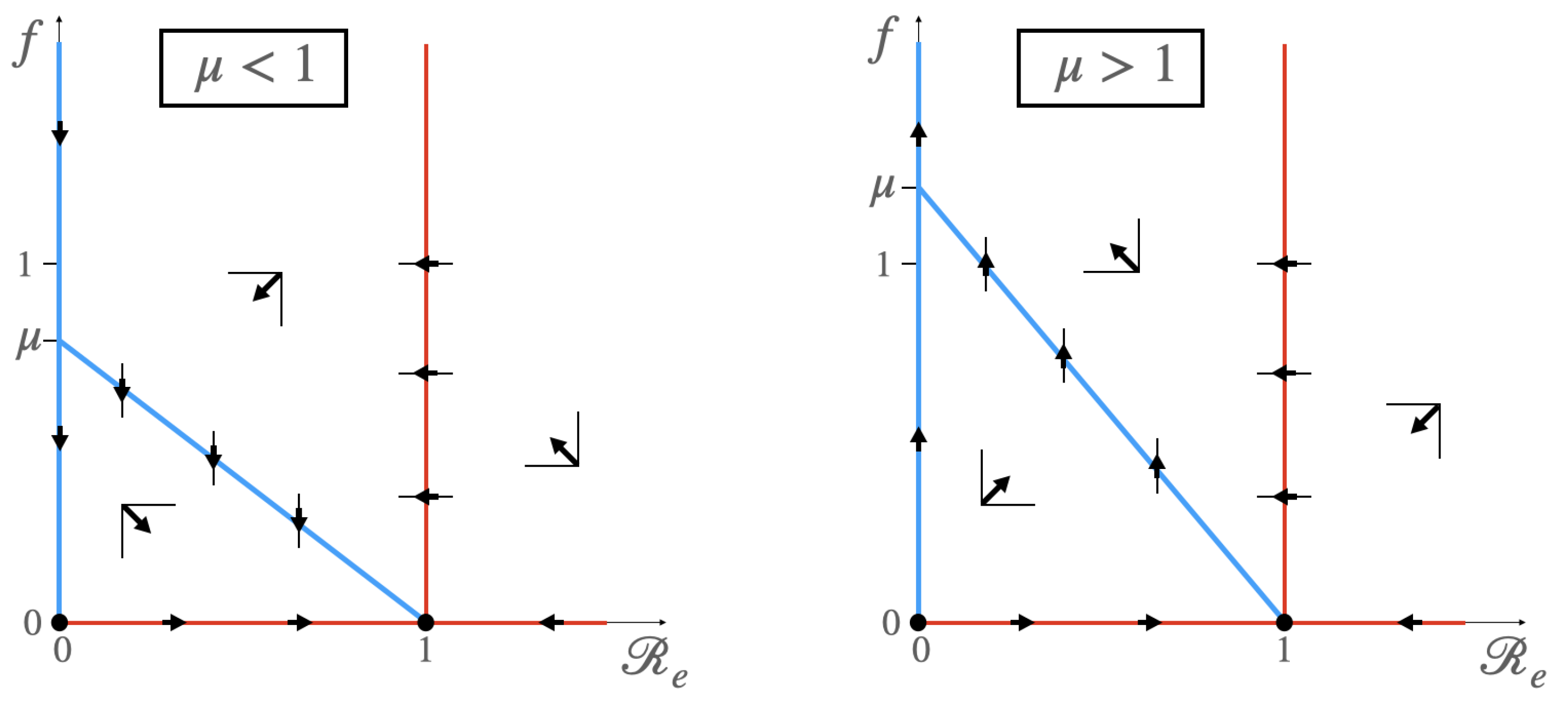
In what follows, we will use a composite variable, denoted by f, which is $\mathbf{B}(I/N)$, the so-called force of infection (transition rate from susceptible to infectious), multiplied by the length of the infectious period ${\gamma }^{-1}$. Thus, f is interpreted as the force (of infection) applied during the specific time (period of infectivity). This fits well with the mechanical concept of impulse (of contagion); that is, f represents the contagion impulse of a generation of active cases.

3.1.1. Case ${\mathbf{F}}_{\oplus }=0$

Theorem 1.

Given (1), the pair effective reproductive number ${\mathcal{R}}_e(·):=(\mathbf{B}/\gamma )(S/N)$ and contagion impulse $f(·):=(\mathbf{B}/\gamma )(I/N)$ satisfy the following planar system:

$$\left\{\begin{array}{ccc}{\mathcal{R}}_e^{\prime }& =& -\gamma \mu \left\{{\mathcal{R}}_e-[1+f/\mu ]\right\}{\mathcal{R}}_e\hfill \\ f^{\prime }& =& +\gamma (1-\mu )({\mathcal{R}}_e-1)f.\hfill \end{array}\right.$$

(2)

Remark 1.

Let us note that ${\mathcal{R}}_e$ (resp. f) corresponds to the number of effective contacts that an individual (anyone in the population) can have with the susceptible group (resp. infective group) during a period of infectiousness. The factor $\mathbf{B}/\gamma$ connects the variables ${\mathcal{R}}_e$ and f through the relationship ${\mathcal{R}}_e·I=f·S$, equality that reflects two ways of counting the number of contacts that occur in the population in which one of the individuals ends up being infected. Another way of expressing the relationship is as a reading of proportion (equality between ratios), that is, ${\mathcal{R}}_e:f=S:I$. Let us also note that if in (2) we change the time variable $\tau =\gamma t$ (i.e., the infectiousness period as a unit of time), the γ parameter disappears in both equations.

Proof of Theorem 1. 

(Considering ${\mathbf{F}}_{\oplus }=0$ in the first equation of the system (1) and first amplifying by ${\gamma }^{-1}(S/N)$ and then summing $\mathbf{B}(S^{\prime }/N)/\gamma$, we obtain the following:

$${\mathbf{B}}^{\prime }\frac{S}{\gamma N}+\frac{\mathbf{B}}{\gamma }\frac{S^{\prime }}{N}=-\mu \gamma ({\mathcal{R}}_e-1)\mathbf{B}\frac{S}{\gamma N}+\frac{\mathbf{B}}{\gamma }\frac{S^{\prime }}{N}.$$

Now, expressing the left-hand side as the derivative of a product and on the right-hand side using for $S^{\prime }$ the second Equation (1), we conclude the following expression:

$${\left(\frac{\mathbf{B}}{\gamma }\frac{S}{N}\right)}^{\prime }=-\mu \gamma ({\mathcal{R}}_e-1)\left(\frac{\mathbf{B}}{\gamma }\frac{S}{N}\right)-\gamma \left(\frac{\mathbf{B}}{\gamma }\frac{S}{N}\right)\left(\frac{\mathbf{B}}{\gamma }\frac{I}{N}\right).$$

Finally, by making substitutions ${\mathcal{R}}_e=(\mathbf{B}/\gamma )(S/N)$ and $f=(\mathbf{B}/\gamma )(I/N)$, there follows, via factorization by ${\mathcal{R}}_e$ on the right-hand side, the first Equation (2).

Concerning f, note that $\gamma Nf=\mathbf{B}I$, so deriving $\gamma N{f}^{\prime }={\mathbf{B}}^{\prime }I+\mathbf{B}{I}^{\prime }$. Then, $\gamma N{f}^{\prime }=-\mu \gamma ({\mathcal{R}}_e-1)\mathbf{B}I+\mathbf{B}\gamma ({\mathcal{R}}_e-1)I$. Dividing by $\gamma N$, we have $f^{\prime }=\{-\mu \gamma ({\mathcal{R}}_e-1)$$+\gamma ({\mathcal{R}}_e-1)\left)\right\}f$, and therefore, factoring by $\gamma ({\mathcal{R}}_e-1)$, we arrive at the second system Equation (2). □

Then, considering that the case of interest is ${\mathcal{R}}_0>1$, we have that as long as the reaction coefficient exceeds the contagion impulse, i.e., $\mu >f$, ${\mathcal{R}}_e$ is decreasing (${\mathcal{R}}_e^{\prime }<0$).

The Jacobian matrix associated with (2) is as follows:

$$\mathcal{J}=\gamma \left(\begin{array}{cc}{a}_{11}& {\mathcal{R}}_e\\ (1-\mu )f& -(1-\mu )\end{array}\right)$$

with $a_{11}=-\mu \{2{\mathcal{R}}_e-[1+f/\mu ]\}$. Moreover, this system has only two equilibria $({\mathcal{R}}_e,f)$, namely, $(0,0)$ and $(1,0)$.

Theorem 2.

Concerning the equilibria associated with the system (2), there are two possible configurations:

(a) 

If $\mu <1$, then $(0,0)$ is a saddle point, and $(1,0)$ is an attractor node.

(b) 

If $\mu >1$, then $(0,0)$ is a repulsor, and $(1,0)$ is a saddle point.

Remark 2.

This result tells us that, in the ideal case of ${\mathbf{F}}_{\oplus }=0$, there is not a contrary force for the mitigation implemented, and there are two long-term possibilities concerning ${\mathcal{R}}_e$. If $\mu <1$ (let us call it weak mitigation reaction), then ${\mathcal{R}}_e$ will go lower than level 1, but in the long term, it will grow and will approach the said level. Now, if $\mu >1$ (let us say strong mitigation reaction), then ${\mathcal{R}}_e$ not only lowers the barrier to value one but also goes to zero out in infinite time.

Proof of Theorem 2. 

Regarding (a), note that $\mathcal{J}(0,0)$ is lower triangular with the eigenvalues $\gamma \mu$ and $-\gamma (1-\mu )$. At the same time, $\mathcal{J}(1,0)$ is upper triangular with the eigenvalues $-\gamma \mu$ and $-\gamma (1-\mu )$. The proof of (b) follows by observation of the change of sign of the factor $(1-\mu )$ in the respective eigenvalues. □

Note that a point $Q({\mathcal{R}}_e,f)$ on a certain trajectory in the phase space of the origin $P(0,0)$ determines an angle $\theta$ formed by the segment $\overline{PQ}$ concerning the axis ${\mathcal{R}}_e$, which satisfies the following:

$$tan\left(\theta \left(t\right)\right)=f/{\mathcal{R}}_e=I\left(t\right)/S\left(t\right).$$

When $\mu <1$, we have that $\theta \to 0$ if $t\to \infty$ (see Figure 1 and Figure 2) so that $tan\left(\theta \right)\to 0$ and as $S(·)$ is a bounded variable, necessarily $I\left(t\right)\to 0$. Similarly, if the case is $\mu >1$, then $\theta \to \pi /2$ if $t\to \infty$ (see Figure 1 and Figure 3) so that $tan\left(\theta \right)\to \infty$ and as $I(·)$ is a bounded variable, necessarily $S\left(t\right)\to 0$, metaphorically indicating that the epidemic is terminated by fuel agorism.

3.1.2. Case ${\mathbf{F}}_{\oplus }\ne 0$

Let us go back to (1) assuming the following condition:

$${\mathbf{F}}_{\oplus }=\nu ({\mathbf{B}}_{*}-\mathbf{B}).$$

This expression assumes that the population, in the presence of a non-zero reaction factor, exhibits a secondary response termed ‘restoration’, characterized by elements of depletion or resistance, leading to reduced adherence. This secondary response occurs at a rate that increases the further the transmission rate deviates from its intrinsic value ${\mathbf{B}}_{*}$ or ‘normality’, towards which it naturally seeks to revert.

The condition that must be fulfilled for ${\mathbf{B}}^{\prime }=0$, e.g., if we ask for a minimum, is ${\mathbf{F}}_{\oplus }={\mathbf{F}}_{\ominus }$, in which the pair $Q:=(\mathbf{B},{\mathcal{R}}_e)$ belongs to the following segment:

$$\mathcal{L}:{\mathcal{R}}_e=1+\frac{\nu }{\mu \gamma }\left\{{\mathbf{B}}_{*}-\mathbf{B}\right\},\mathbf{B}\in [0,{\mathbf{B}}_{\infty }].{\mathbf{B}}_{\infty }:={\mathbf{B}}_{*}+\mu \gamma /\nu .$$

We are interested in the dynamics of the pair $Q(·)$ with respect to its relative position concerning $\mathcal{L}$ (see Figure 4), particularly its dynamics inside the triangle bounded by the axes ${\mathcal{R}}_e=0$, $\mathbf{B}=0$, and the straight line $\mathcal{L}$. This triangular region is a confinement for the trajectories of $Q(·)$ since in its legs $({\mathcal{R}}_e^{\prime },{\mathbf{B}}^{\prime })=(0,0)$, and as will be proved, if it is in $\mathcal{L}$, the dynamics point to its interior.

Let us note that the pair $({\mathbf{B}}_{*},1)$ belongs to $\mathcal{L}$. However, initially, $Q_0:=Q\left(0\right)=({\mathbf{B}}_{*},{\mathcal{R}}_0)$, so $Q_0$ is above $\mathcal{L}$ since the intrinsic assumption is ${\mathcal{R}}_0>1$. Furthermore, ${\mathbf{B}}^{\prime }\left(0\right)=({\mathbf{F}}_{\oplus }\left(0\right)$ $- {\mathbf{F}}_{\ominus }\left(0\right)){\mathbf{B}}_{*}=-\mu \gamma ({\mathcal{R}}_0-1){\mathbf{B}}_{*}<0$ and

$${\mathcal{R}}_e^{\prime }\left(0\right)={\gamma }^{-1}\{{\mathbf{B}}^{\prime }\left(0\right)S\left(0\right)+\mathbf{B}\left(0\right)S^{\prime }\left(0\right)\}/N=-\{\mu ({\mathcal{R}}_0-1)+{\mathcal{R}}_0\}{\mathbf{B}}_{*}/N<0,$$

so $Q_0$ shows a forward direction to the left and downward. In the two components of the motion, it starts approaching $\mathcal{L}$, as seen in Figure 4.

On the other hand, if a first-time $\tau >0$ exists in which $Q_1:=Q\left(\tau \right)\in \mathcal{L}$, then ${\mathbf{B}}^{\prime }\left(\tau \right)=0$ and

$${\mathcal{R}}_e^{\prime }\left(\tau \right)=-\gamma {\mathcal{R}}_e\left(\tau \right)·f\left(\tau \right)<0.$$

This shows a period after time $\tau$, where $Q\left(t\right)$ is below the straight line $\mathcal{L}$.

Once a point $Q(·)$ is below the straight line $\mathcal{L}$, it is always forced by the left to approach $\mathcal{L}$ (because ${\mathbf{B}}^{\prime }>0$); if it reaches $\mathcal{L}$, it receives an impulse to descend (because ${\mathbf{R}}_e^{\prime }<0$ and ${\mathbf{B}}^{\prime }=0$) and returns to below $\mathcal{L}$. In summary, when entering the triangle, the trajectory of $Q(·)$ (see Figure 4) does not leave it and makes a trajectory of constant advance to the right. In the vertical component, it goes down (potentially with oscillations) and ultimately converges (in infinite time) to the point $(0,{\mathbf{B}}_{\infty })$.

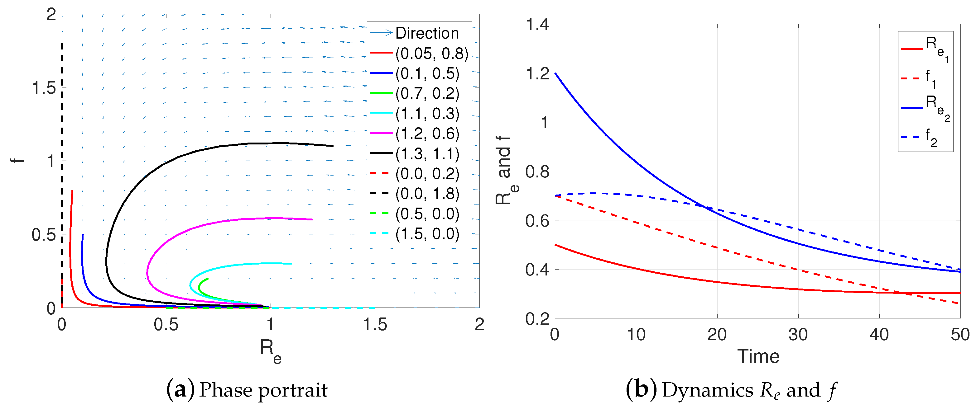
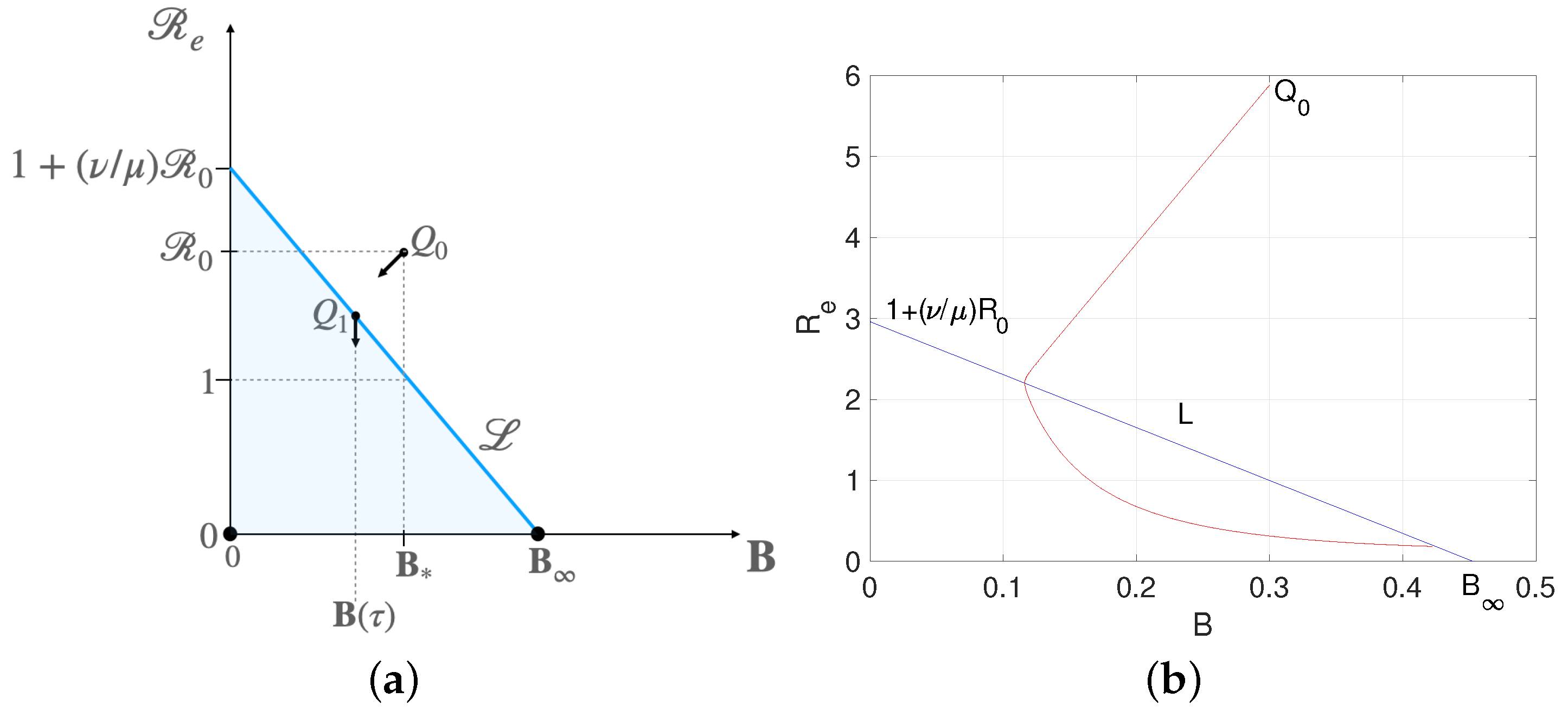
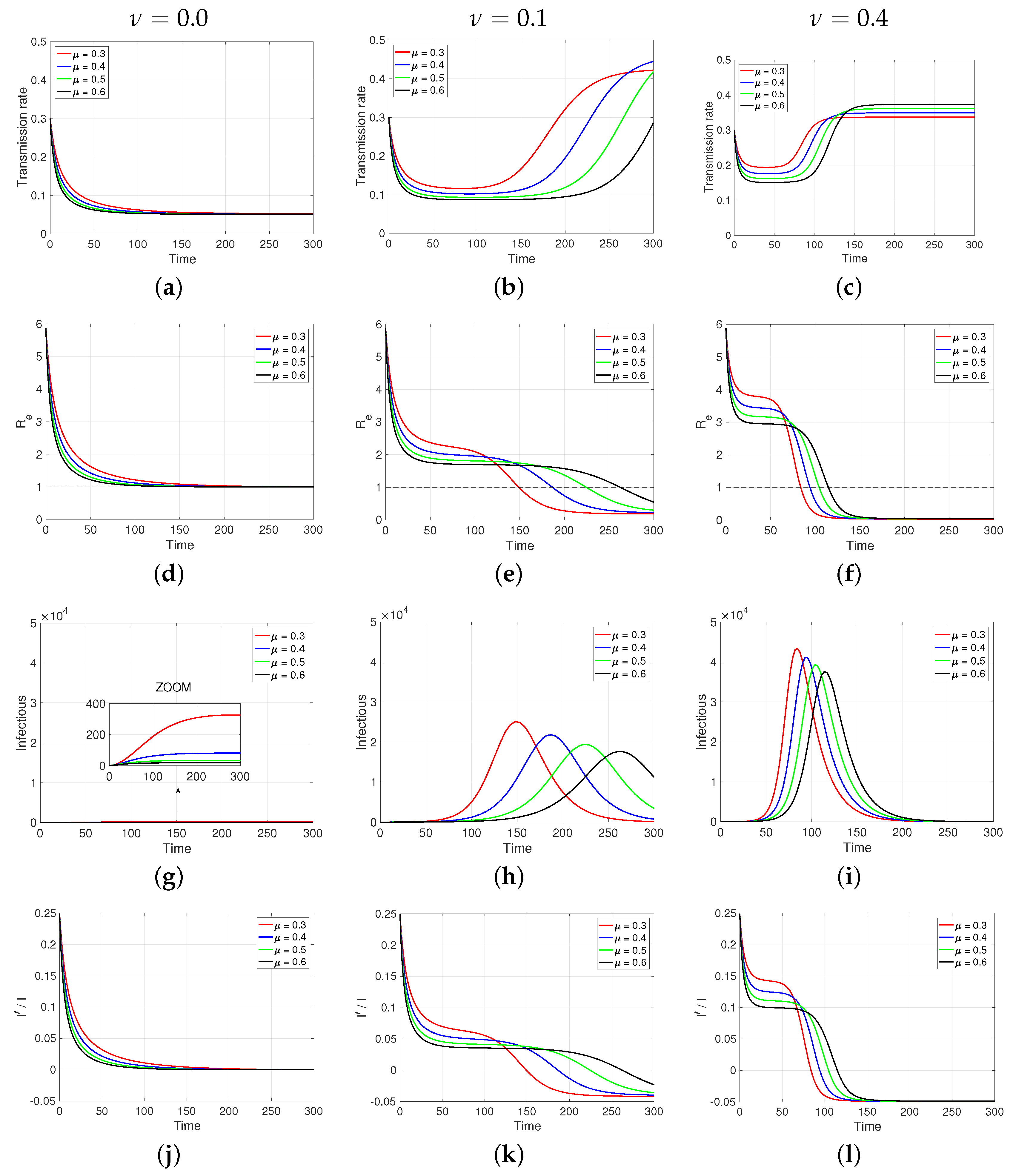
3.2. Numerical Results

As we already know, in the case without the restoration coefficient $\nu =0$, we have that the reaction obtains ${\mathcal{R}}_e$ asymptotically down to the value one (see Figure 5d), and therefore, since ${\mathbf{B}}^{\prime }=\mu \gamma ({\mathcal{R}}_e-1)$, we have that ${\mathbf{B}}^{\prime }$ tends towards zero (Figure 5a). Then, as expected, in the absence of restoring pressure, we have that the infection, in terms of the size of the infectious group, develops very late and at relatively narrow levels, which negatively correlates with the reaction coefficient $\mu$ (Figure 5g).

In the graph matrix that is in Figure 5, when comparing the last two columns, that is, $\nu =0.1$ and $\nu =0.4$, we see that the effect of a lower restoration coefficient results in longer valleys where $\mathbf{B}$ minima are extended (Figure 5b,c), which in turn results in reproductive number drops to a value closer to one above, and longer (Figure 5e,f). Although ${\mathcal{R}}_e$ is lower than in subsequent periods, this is because susceptibles are infected more slowly, as evident in the infectious group graphs (Figure 5c,h).

Fixing $\nu$ and concentrating on the effect of $\mu$, the reaction coefficient, it is observed that at, higher values, the rate drops to lower levels but recovers to higher values, acting as compensation. The most significant work, to flatten and postpone the peak of the curve of new daily cases, i.e., its control work, is achieved with higher reaction coefficients. However, it is essential to note that this control is in the flat zone, even with values of the effective reproductive number greater than one.

4. Discussion and Conclusions

We have investigated the dynamics of a high-risk infectious disease, such as the COVID-19 transmission, using a modified SIR model incorporating human behavior through the so-called reaction (associated with good conduct due to the decision to carry out mitigation and its compliance) and restitution (associated with misconduct due to non-compliance) factors. Our analysis revealed that the effective reproductive number and the contagion impulse are crucial in understanding the spread of the virus. When analogizing a contagion process with the spread of a forest fire, two aspects are immediate to evaluate its state and growth potential, the combustible biomass (susceptible individuals) and the biomass in combustion (active individuals). However, these variables are not enough; it is necessary to consider parameters such as tree spacing, ambient humidity, or airspeed. For a contagion represented by a SIR model, this determining information is given by $\mathbf{B}$ and $\gamma$ parameters. It is important to have a quality-quantity indicator of the fuel and the burning material, in our case a “susceptible potential” and an “infectious potential”. Given contacts, transmissibility, number of susceptible individuals, and exposure time to an ineffective one, this indicator is ${\mathcal{R}}_e$. From the perspective of the active group, this quality–quantity is measured by f, the contagion impulse. Thus, thinking and modeling in terms of ${\mathcal{R}}_e$ and f have emerged to be important in terms of monitoring, planning needs, evaluation of control, and anticipation via trends.

We found that populations with high adherence to mitigation measures can maintain the effective reproductive number close to one, effectively controlling the epidemic’s spread. The model also demonstrated that when the reaction coefficient is higher than the contagion impulse, ${\mathcal{R}}_e$ decreases, highlighting the importance of swift and robust public health responses. Furthermore, our results showed that a restitution factor can create a plateau in Re above one, delaying and lowering the peak of infection. These findings underscore the significance of timely interventions and sustained public health measures to manage and mitigate the impact of COVID-19.

An interesting aspect for populations with a low level of restoration, or in favorable terms, with high adherence, that is, $\nu \sim 0$, is that, early on (with a fraction of infected $I/N\sim 0$), they manage to lower the transmission rate so that $f\sim 0$; the latter implies, according to the first Equation, (2) the following:

$${\mathcal{R}}_e^{\prime }\sim \gamma \mu \{1-{\mathcal{R}}_e\}{\mathcal{R}}_e.$$

That is, it satisfies the logistic equation, which suggests staying close to one as long as they maintain the compliance conditions, since, in this last equation, ${\mathcal{R}}_e=1$ is an equilibrium (i.e., ${\mathcal{R}}_e^{\prime }=0$) that is globally asymptotically stable. This can be observed in the COVID-19 experience in several countries [25,26,27,28].

This is particularly interesting since we are saying that $\mathbf{B}$ has a final equilibrium over the intrinsic equilibrium, which can only be explained by the fact that the prolonged reaction factor changes sign when the reproductive number is below ${\mathcal{R}}_e=1$. However, in reality, the improving epidemiological situation may become an incentive to resume activities (at a greater rate than usual) in terms of contacts and without increasing the transfer of pathogens, that is, in the components of the probabilities that define the transmission rate. However, intuition suggests that this should be temporary and not lead to a new intrinsic equilibrium. In this sense, the model has a caveat in that there should be a condition after which the reaction factor ${\mathbf{F}}_{\ominus }=0$ cancels out.

In real populations, the absence of restitution forces for a long time at an early stage of the development of the disease transmission process ($\nu =0$, see first column of Figure 5) may be a feasible ideal to achieve (e.g., because of good communication policy or a natural fear of contagion). However, experience would show that both the loss of adherence in the first instance and compliance with the mitigating resolutions in the medium and long term seem inevitable. There are multiple reasons for this, highlighting those related to the physiological and psychological health of individuals as well as their economic health, which, by the way, can result in severe social imbalances.

Regarding the fact that, in the medium or long term, $\nu \ne 0$, from the observation in Figure 5e,f, it is essential to note that ${\mathcal{R}}_e$, after a considerable drop, generates a plateau (resembling a constant) at a value higher than one where, although it does not destroy the wave (Figure 5h,i), it does delay and lower its maximum. This aspect is identified for $\mu$ as having higher intensities than expected.

Our study’s strengths include the integration of reaction and restitution factors into the SIR model, offering nuanced insights into COVID-19 transmission dynamics and the impact of mitigation measures. The analytical approach provides a precise characterization of epidemic trends under varying levels of public compliance. However, our study assumes homogeneous population mixing to illustrate our theoretical ideas. A pending challenge to add a pinch of realism is to assume that there is a time lag between the evaluation and the implementation–communication of the mitigating measures, that is, to consider that ${\mathbf{F}}_{\ominus }$, equivalent in our case to ${\mathcal{R}}_e$, in the first Equation (1) has a time delay.

References

1. Gilardino, R.E. Does “flattening the curve” affect critical care services delivery for COVID-19? A global health perspective. Int. J. Health Policy Manag. 2020, 9, 503. [Google Scholar] [CrossRef]
2. Palomo, S.; Pender, J.J.; Massey, W.A.; Hampshire, R.C. Flattening the curve: Insights from queueing theory. PLoS ONE 2023, 18, e0286501. [Google Scholar] [CrossRef]
3. Tashiro, A.; Shaw, R. COVID-19 pandemic response in Japan: What is behind the initial flattening of the curve? Sustainability 2020, 12, 5250. [Google Scholar] [CrossRef]
4. Di Lauro, F.; Kiss, I.Z.; Rus, D.; Della Santina, C. COVID-19 and flattening the curve: A feedback control perspective. IEEE Control Syst. Lett. 2020, 5, 1435–1440. [Google Scholar] [CrossRef]
5. Giannakeas, V.; Bhatia, D.; Warkentin, M.T.; Bogoch, I.I.; Stall, N.M. Estimating the maximum capacity of COVID-19 cases manageable per day given a health care system’s constrained resources. Ann. Intern. Med. 2020, 173, 407–410. [Google Scholar] [CrossRef]
6. Bustan, S.; Nacoti, M.; Botbol-Baum, M.; Fischkoff, K.; Charon, R.; Madé, L.; Simon, J.R.; Kritzinger, M. COVID-19: Ethical dilemmas in human lives. J. Eval. Clin. Pract. 2021, 27, 716–732. [Google Scholar] [CrossRef]
7. Neves, N.M.; Bitencourt, F.B.; Bitencourt, A.G. Ethical dilemmas in COVID-19 times: How to decide who lives and who dies? Rev. Assoc. Med. Bras. 2020, 66, 106–111. [Google Scholar] [CrossRef]
8. Holleran, S. Dying Apart, Buried Together: COVID-19, Cemeteries and Fears of Collective Burial. In Death’s Social and Material Meaning Beyond the Human; Bristol University Press: Bristol, UK, 2024; pp. 100–113. [Google Scholar]
9. Hamid, W.; Jahangir, M.S. Dying, death and mourning amid COVID-19 pandemic in Kashmir: A qualitative study. OMEGA-J. Death Dying 2022, 85, 690–715. [Google Scholar] [CrossRef]
10. Raffaetà, R. Another Day in Dystopia. Italy in the Time of COVID-19. Med. Anthropol. 2020, 39, 371–373. [Google Scholar] [CrossRef]
11. Calmon, M. Considerations of coronavirus (COVID-19) impact and the management of the dead in Brazil. Forensic Sci. Int. Rep. 2020, 2, 100110. [Google Scholar] [CrossRef]
12. Çakan, S. Dynamic analysis of a mathematical model with health care capacity for COVID-19 pandemic. Chaos Solitons Fractals 2020, 139, 110033. [Google Scholar] [CrossRef]
13. Gutiérrez-Aguilar, R.; Córdova-Lepe, F.; Muñoz-Quezada, M.T.; Gutiérrez-Jara, J.P. Model for a threshold of daily rate reduction of COVID-19 cases to avoid hospital collapse in Chile. Medwave 2020, 20, e7871. [Google Scholar] [CrossRef]
14. Jiliberto, R.R. Deja a la Estructura Hablar: Modelización y Análisis de Sistemas Naturales, Sociales y Socioecológicos; Ediciones UM: Murcia, Spain, 2020. [Google Scholar]
15. Canals, M.; Cuadrado, C.; Canals, A. COVID-19 in Chile: The usefulness of simple epidemic models in practice. Medwave 2021, 21, e8119. [Google Scholar] [CrossRef]
16. Adiga, A.; Dubhashi, D.; Lewis, B.; Marathe, M.; Venkatramanan, S.; Vullikanti, A. Mathematical models for COVID-19 pandemic: A comparative analysis. J. Indian Inst. Sci. 2020, 100, 793–807. [Google Scholar] [CrossRef]
17. Rojas-Vallejos, J. Strengths and limitations of mathematical models in pandemics—The case of COVID-19 in Chile. Medwave 2020, 20, e7876. [Google Scholar] [CrossRef]
18. Manca, D.; Caldiroli, D.; Storti, E. A simplified math approach to predict ICU beds and mortality rate for hospital emergency planning under COVID-19 pandemic. Comput. Chem. Eng. 2020, 140, 106945. [Google Scholar] [CrossRef]
19. Biggerstaff, M.; Cowling, B.J.; Cucunubá, Z.M.; Dinh, L.; Ferguson, N.M.; Gao, H.; Hill, V.; Imai, N.; Johansson, M.A.; Kada, S.; et al. Early insights from statistical and mathematical modeling of key epidemiologic parameters of COVID-19. Emerg. Infect. Dis. 2020, 26, e1–e14. [Google Scholar] [CrossRef]
20. Thompson, R.N.; Hollingsworth, T.D.; Isham, V.; Arribas-Bel, D.; Ashby, B.; Britton, T.; Challenor, P.; Chappell, L.H.; Clapham, H.; Cunniffe, N.J.; et al. Key questions for modelling COVID-19 exit strategies. Proc. R. Soc. B 2020, 287, 20201405. [Google Scholar] [CrossRef]
21. Gostic, K.M.; McGough, L.; Baskerville, E.B.; Abbott, S.; Joshi, K.; Tedijanto, C.; Kahn, R.; Niehus, R.; Hay, J.A.; De Salazar, P.M.; et al. Practical considerations for measuring the effective reproductive number, Rt. PLoS Comput. Biol. 2020, 16, e1008409. [Google Scholar] [CrossRef]
22. Flaxman, S.; Mishra, S.; Gandy, A.; Unwin, H.J.T.; Mellan, T.A.; Coupland, H.; Whittaker, C.; Zhu, H.; Berah, T.; Eaton, J.W.; et al. Estimating the effects of non-pharmaceutical interventions on COVID-19 in Europe. Nature 2020, 584, 257–261. [Google Scholar] [CrossRef]
23. Córdova-Lepe, F.; Vogt-Geisse, K. Adding a reaction-restoration type transmission rate dynamic-law to the basic SEIR COVID-19 model. PLoS ONE 2022, 17, e0269843. [Google Scholar] [CrossRef]
24. Córdova-Lepe, F.; Gutiérrez-Jara, J.P. A dynamic reaction-restore-type transmission-rate model for COVID-19. WSEAS Trans. Biol. Biomed. 2024, 21, 118–130. [Google Scholar] [CrossRef]
25. Huisman, J.S.; Scire, J.; Angst, D.C.; Li, J.; Neher, R.A.; Maathuis, M.H.; Bonhoeffer, S.; Stadler, T. Estimation and worldwide monitoring of the effective reproductive number of SARS-CoV-2. eLife 2022, 11, e71345. [Google Scholar] [CrossRef]
26. Bsat, R.; Chemaitelly, H.; Coyle, P.; Tang, P.; Hasan, M.R.; Al Kanaani, Z.; Al Kuwari, E.; Butt, A.A.; Jeremijenko, A.; Kaleeckal, A.H.; et al. Characterizing the effective reproduction number during the COVID-19 pandemic: Insights from Qatar’s experience. J. Glob. Health 2022, 12, 05004. [Google Scholar] [CrossRef]
27. Bokányi, E.; Vizi, Z.; Koltai, J.; Röst, G.; Karsai, M. Real-time estimation of the effective reproduction number of COVID-19 from behavioral data. Sci. Rep. 2023, 13, 21452. [Google Scholar] [CrossRef]
28. Hridoy, A.E.E.; Tipo, I.H.; Sami, M.S.; Babu, M.R.; Ahmed, M.S.; Rahman, S.M.; Tusher, S.M.S.H.; Rashid, K.J.; Naim, M. Spatio-temporal estimation of basic and effective reproduction number of COVID-19 and post-lockdown transmissibility in Bangladesh. Spat. Inf. Res. 2022, 30, 23–35. [Google Scholar] [CrossRef]
Figure 1. Isoclines, direction field, and equilibria are defined by the system (1) for the cases μ < 1 (on the left) and μ > 1 (on the right). In blue (resp. in red), the solution set of R e = 0 (resp.  f = 0 ).
Mathematics 12 01793 g001
Figure 2. Case μ < 1 with μ = 0.4 , ν = 0 , and γ = 0.051 . (a) Field and phases for Impulse vs. Effective Reproductive No., f vs. R e , and (b) Impulse and Effective Reproductive No. as functions of time for initial conditions R e 1 ( 0 ) = 0.5 , R e 2 ( 0 ) = 1.2 , and f 1 ( 0 ) = f 2 ( 0 ) = 0.7 .
Mathematics 12 01793 g002
Figure 3. Case μ > 1 with μ = 1.4 , ν = 0 , and γ = 0.051 . (a) Field and phases for Impulse vs. Effective Reproductive No., f vs. R e , and (b) Impulse and Effective Reproductive No. as functions of time for initial conditions R e 1 ( 0 ) = 0.5 , R e 2 ( 0 ) = 1.2 , and f 1 ( 0 ) = f 2 ( 0 ) = 0.7 .
Mathematics 12 01793 g003
Figure 4. The behavior of variables B and R e is associated with system (1). (a) Dynamics of the pair ( B , R e ) with respect to its relative position concerning L . For (b), ν = 0.1 and μ = 0.3 . Conditions initials: S ( 0 ) = 99 , 999 , I ( 0 ) = 1 , R ( 0 ) = 0 , and β ( 0 ) = 0.3 . γ = 0.051 and N = 100 , 000 were considered. Q 0 = ( 0.3 , 5.8823 ) , 1 + ( ν / μ ) R 0 = 2.9608 , and B = 0.4530 .
Mathematics 12 01793 g004
Figure 5. Simulations of Equation (1) for different values of ν and μ . (al) Conditions initials: S ( 0 ) = 99 , 999 , I ( 0 ) = 1 , R ( 0 ) = 0 , and B ( 0 ) = B * = 0 . 3 . γ = 0.051 and N = 100 , 000 were considered.
Mathematics 12 01793 g005
Disclaimer/Publisher’s Note: The statements, opinions and data contained in all publications are solely those of the individual author(s) and contributor(s) and not of MDPI and/or the editor(s). MDPI and/or the editor(s) disclaim responsibility for any injury to people or property resulting from any ideas, methods, instructions or products referred to in the content.