Article

A Dual-Competition-Based Particle Swarm Optimizer for Large-Scale Optimization

1
Postgraduate of Faculty of Mechanical Engineering, RWTH Aachen University, 52062 Aachen, Germany
2
Sino-German College of Applied Sciences, Tongji University, Shanghai 200092, China
*
Author to whom correspondence should be addressed.
Mathematics 2024, 12(11), 1738; https://doi.org/10.3390/math12111738
Submission received: 30 April 2024 / Revised: 29 May 2024 / Accepted: 30 May 2024 / Published: 3 June 2024

Abstract

:
Large-scale particle swarm optimization (PSO) has long been a hot topic due to the following reasons: Swarm diversity preservation is still challenging for current PSO variants for large-scale optimization problems, resulting in difficulties for PSO in balancing its exploration and exploitation. Furthermore, current PSO variants for large-scale optimization problems often introduce additional operators to improve their ability in diversity preservation, leading to increased algorithm complexity. To address these issues, this paper proposes a dual-competition-based particle update strategy (DCS), which selects the particles to be updated and corresponding exemplars with two rounds of random pairing competitions, which can straightforwardly benefit swarm diversity preservation. Furthermore, DCS confirms the primary and secondary exemplars based on the fitness sorting operation for exploitation and exploration, respectively, leading to a dual-competition-based swarm optimizer. Thanks to the proposed DCS, on the one hand, the proposed algorithm is able to protect more than half of the particles from being updated to benefit diversity preservation at the swarm level. On the other hand, DCS provides an efficient exploration and exploitation exemplar selection mechanism, which is beneficial for balancing exploration and exploitation at the particle update level. Additionally, this paper analyzes the stability conditions and computational complexity of the proposed algorithm. In the experimental section, based on seven state-of-the-art algorithms and a recently proposed large-scale benchmark suite, this paper verifies the competitiveness of the proposed algorithm in large-scale optimization problems.

1. Introduction

Particle swarm optimization (PSO) has been widely applied in engineering optimization in past decades due to their simplicity and efficiency [1,2,3,4,5]. On the one hand, PSO shows better robustness and computational efficiency in comparison to gradient-based algorithms [6]. On the other hand, in comparison to many existing evolutionary algorithms (e.g., genetic algorithms [7], ant colony optimizer [8], teaching–learning-based optimization [9], and brain storm optimization [10]), PSO has the advantages of easy implementation, efficient parameter tuning, and flexible manners of hybridization with other optimization methods [11].
However, PSO has been found to be inefficient in solving large-scale optimization problems (LSOPs). Without losing generality, the LSOP mentioned in this paper aims to minimize a given function, which can be formulated by (1).
m i n f ( x ) , x = [ x 1 , , x d , , x D ] a n d D 100
where D is the dimensionality of the considered optimization function, and x d denotes the d th dimension of the decision vector. Note that (i) f ( x ) is a continuous black box function with boundary constraints on the decision variables, and (ii) the dimensionality considered in this paper is up to 1000, which is a common setting in relevant research. The main reason for this is that PSO cannot effectively conduct swarm diversity preservation when solving LSOPs and is thus easily trapped in local optima. To be specific, this is caused by PSO’s exemplar selection mechanism: the g b e s t and p b e s t in PSO are of poor diversity during the optimization process [12], since it is difficult to locate more promising solutions based on the current swarm. Therefore, the swarm tends to converge to the local optimum, resulting in premature convergence. On the other hand, limited computing resources only allow PSO to search part of the search spaces [13].
Targeting these two issues, a large body of research has been put forward to improve PSO for LSOPs. The mainstream of the current work can be roughly divided into three categories: exemplar diversification, decoupled learning, and hybridization of PSO and other techniques.
The methods in the first category propose to enhance the diversity of the exemplars for the updated particles [12,13,14,15,16,17,18,19], thereby improving PSO’s balance between exploration and exploitation. For instance, the competitive swarm optimizer (CSO) assigns each updated particle a distinguishing exemplar [12], the social learning particle swarm optimizer (SLPSO) allows the updated particles to learn all of the particles that are better than the specific updated particles [14], and the level-based learning swarm optimizer (LLSO) randomly selects two exemplars for each updated particle [13]. Through these means, the exemplars of the updated particles can be hugely diversified in comparison to the basic PSO, which leads to benefits in diversity preservation.
The approaches in the second category focus on decoupling the convergence learning component and the diversity learning component in the velocity update structure for the basic PSO [1,20,21]. Afterwards, such algorithms adjust the parameters in the diversity learning component to control swarm diversity. Consequently, an important design factor in such methods is the study of the local diversity measurements to be adopted as the basis of the diversity learning component, such as the local sparseness degree [1].
For hybrid PSO, the main idea is to utilize other optimization techniques to enhance PSO in diversity preservation. For instance, chaotic local search [22] and the memetic algorithm [23] can be adopted to promote PSO in local search for diversity preservation. One possible solution that can be employed to help diversity preservation is to update the rules of the simulated annealing algorithm [24] and the genetic algorithm [25].
However, these methods still show room for further improvement. First, for the methods with exemplar diversification strategies, the early attempts, such as CSO and SLPSO, fail at simultaneously diversifying the two exemplars for the updated particles [13]. Recent methods, such as LLSO, are ineffective in preserving promising particles, consequently resulting in adverse impacts on diversity preservation. Furthermore, recent methods often introduce additional operators for exemplar selection, leading to extra parameter tuning tasks and computational complexity. Second, the approaches with decoupled learning mechanisms show poor ability in preserving promising particles; on the other hand, they are computationally complex in evaluating the local diversity information, which should impose constraints on their performance if the computation resources are limited. In summary, one can find that both the recent methods in the two categories fail at effectively protecting promising particles from being updated for diversity preservation and simplifying the complexity of the algorithm. Third, for the hybrid PSO variants, extra parameter tuning tasks will be required due to the introduction of other optimization operators [12]. Therefore, diversity preservation for PSO in LSOPs is still challenging.
To address this issue, this paper aims to design novel learning mechanisms for both diversity preservation and efficient exemplar selection to improve PSO in both performance and efficiency. To this end, a novel variant of PSO is proposed, and the main contributions of this paper are listed as follows:
  • To enhance the diversity preservation ability of PSO, this paper puts forward an efficient dual-competition-based learning mechanism, which is able to efficiently help diversify the exemplars of the updated particles and preserve promising particles. Therefore, the proposed mechanism can significantly enhance PSO in diversity preservation.
  • Based on the proposed dual-competition-based learning mechanism, a novel variant of PSO for LSOPs is proposed, referred to as the dual-competition-based particle swarm optimizer (PSO-DC).
  • Comprehensive theoretical analysis and experiments are conducted, which demonstrate the competitiveness of the proposed algorithm from both theoretical and experimental perspectives.
The subsequent sections of this work are structured as follows: Section 2 provides a review of the current improvements in PSO for LSOPs. Section 3 presents the details of the proposed dual-competition-based learning mechanism. Section 4 provides a theoretical analysis of the computational complexity and the searching characteristics of the proposed algorithm. Section 5 experimentally tests the performance of the proposed algorithm. Finally, we conclude this paper and highlight directions for future work in Section 6.

2. Related Work

In this section, to provide readers with a comprehensive understanding of the developments in PSO for LSOPs, a deliberated review of the current mainstream improvements in PSO for LSOPs is presented, including the cooperative coevolution-based PSO variants, exemplar diversification-based PSO variants, decoupled learning-based PSO variants, and hybrid PSO variants.

2.1. CC-Based Methods for Dimensionality Reduction

The cooperative coevolution (CC) framework was first put forward by Bergh et al. and aims to solve LSOPs in low-dimensional spaces to reduce the difficulties that PSO has with diversity preservation [26], as evidenced by CCPSO- S H and CCPSO- S K . These two methods randomly divide the whole decision vector into K sub-components, where K is predefined by users. Then, PSO is utilized to simultaneously optimize the decomposed sub-components.
However, CC-based methods are ineffective at solving LSOPs that involve complex interactions among the decision variables. To solve this problem, randomness-based variable grouping methods and analysis-based differential grouping methods have been proposed in past decades. Randomness-based variable grouping methods—such as CCPSO [27], CCPSO2 [28], and CGPSO [29]—propose to dynamically and randomly conduct variable grouping and update the grouping scenarios based on improvements in the overall performance to promote the grouping of variables with interactions into the same components. Second, for methods based on variable interaction analysis, a baseline can be found in differential grouping (DG) [30], which directly analyzes the interactions between variables based on the fitness variation. On the basis of DG, different versions of DG have been put forward for specific problems and grouping acceleration, such as DG2 [31], RDG [32], RDG2 [33], ERDG [34], MDG [35], and several kinds of improved DG [36,37].
Despite the success of the current CC-based algorithms, such methods show the following drawbacks [1,13]: (i) grouping accuracy cannot be ensured; (ii) the process of variable grouping is time consuming; and (iii) it is difficult to set proper context vectors to balance the exploration and exploitation of the CC-based algorithms. Therefore, researchers tend to design novel exemplar diversification strategies and learning structures for PSO to directly enhance it in diversity preservation for improving its search efficiency.

2.2. Exemplar Diversification-Based Methods

As discussed in Section 1, such algorithms pay attention to diversifying the exemplars of the updated particles, and the main idea is to modify the topologies among particles.
Early typical works can be found in CSO [12] and SLPSO [14]. On the one hand, both of them employ the current position as the exemplars for the updated particles, where the current positions are of higher diversity than the g b e s t and p b e s t in basic PSO. On the other hand, CSO allows half of the particles to be kept without any operation at each generation, which is able to significantly benefit diversity preservation [12,13]. Nevertheless, the second exemplar for each updated particle in CSO and SLPSO is the mean position of the whole swarm, resulting in adverse impacts on diversity preservation [13]. To solve this issue, different kinds of exemplar selection strategies have been proposed in recent years, as evidenced by level-based exemplar selection [13,16,38], randomness-based exemplar selection [17,18], and superiority combination exemplar selection [19]. Lan et al. introduced a modified competition mechanism and a two-phase learning strategy [39]. All these methods concentrate on diversifying the exemplars for updated particles to balance convergence and diversity for PSO.
However, although the recently proposed exemplar selection mechanisms have achieved great improvements in diversifying the exemplars in comparison to CSO, they have not shown advantages in preserving promising particles, which is significantly beneficial to diversity preservation, as noted by [1,13].

2.3. Decoupled Learning-Based Methods

Different from exemplar diversification-based methods, decoupled learning-based methods propose to control the diversity with specific parameters. In line with this idea, Li et al. put forward three kinds of PSO variants, namely APSODEE, MAPSODEE, and PSODBCD [1,20,21]. Such methods build on different local diversity measurements, using particles with better local diversity to guide particles with poor local diversity. Zhang et al. have also developed decoupled convergence and diversity learning structures [40], where they update particles with different characteristics for convergence and diversity preservation, respectively.
In general, such methods show good potential in balancing exploration and exploitation. However, additional indicators should be designed to evaluate the local diversity information, leading to issues with respect to computational complexity and local diversity measurement accuracy. Furthermore, such methods are also inefficient in preserving promising particles for diversity enhancement. For example, most of the particles in APSODEE will be updated in the latter half of the optimization process.

2.4. Hybrid Methods

Hybrid methods mainly focus on adopting different optimization techniques to design new particle update strategies for diversity preservation. For example, CGPSO proposes to incorporate chaotic local search into PSO, which can help refine each solution in local search space, thereby benefiting diversity preservation [22]. SA-PSO employs an update rule from the simulated annealing algorithm to help avoid useless particle updates, which favors protecting diversity [24]. HPSOGA designs a diversity enhancement based on genetic operators [25].
However, there exists a distinguishing issue in such methods: extra parameter tuning tasks [12]. The reason for this is that different algorithms contain different parameters. Such extra parameters increase the complexity of the algorithm, which has adverse effect on algorithms’ robustness and generality.

3. Proposed Method

In this section, this paper proposes a novel variant of particle swarm optimizer which can diversify the exemplars for the updated particles, protect the promising particles, and is of low computational cost.
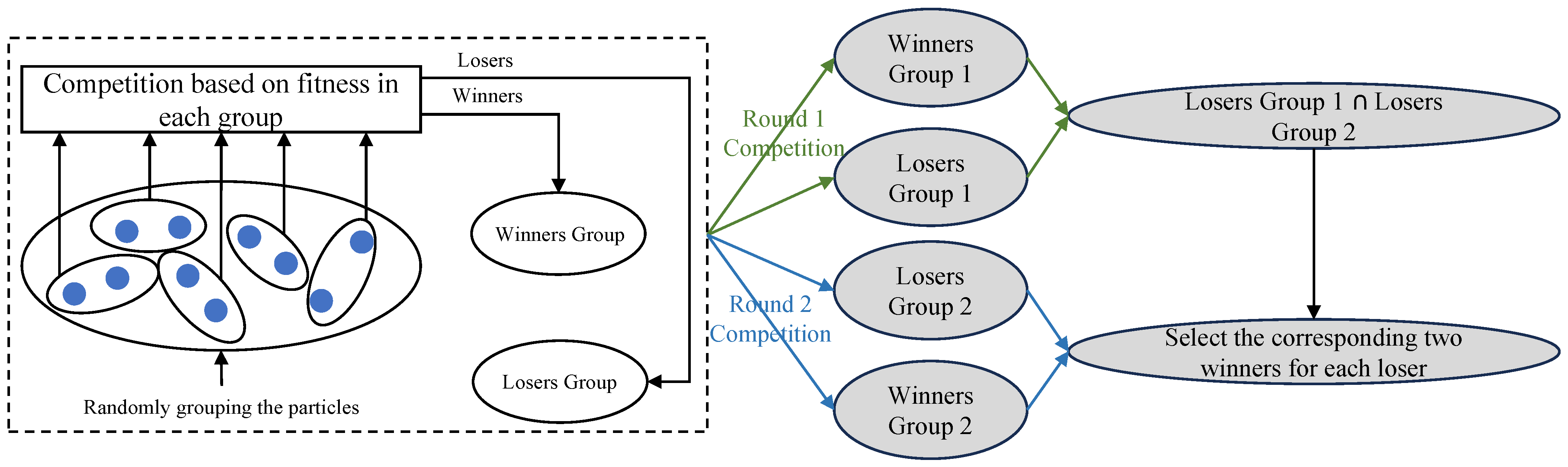
First, the proposed exemplar and updated particle selection method (referred to as the dual-competition-based strategy, DCS) can be illustrated in Figure 1. To be specific, the competition mechanism [12] is independently executed for twice at each generation, leading to two winners groups and two losers groups. Afterwards, the particles to be updated at each generation can be obtained by taking the intersection of the two loser groups, namely, “Losers Group 1” and “Losers Group 2” in Figure 1. Consequently, the exemplars for the obtained particles to be updated are the corresponding winners in “Winners Group 1” and “Winners Group 2”. Here, a brief of the competition mechanism is presented to ensure the integrity of the proposed mechanism: first, a swarm with size N p o p is randomly divided into N p o p / 2 sub-swarms and second, in each sub-swarm, the particle with the better fitness is regarded as the winner and put into the winners group while the other one is put into the losers group.
Second, in order to distinguish the exploitation and exploration exemplars, the two exemplars for each particle are sorted based on their fitness: the better exemplar is adopted as the exploitation exemplar, and the other exemplar is employed as the exploration exemplar. This is inspired by [13]: learning from a more promising exemplar shows advantages in exploitation, while learning from a relatively inferior exemplar tends to explore more regions of the decision space.
Finally, the velocity and position of the particles to be updated are iterated according to (2) and (3), leading to the proposed dual-competition-based particle swarm optimizer (PSO-DC).
v i d ( t + 1 ) = ω v i d ( t ) + r 1 ( e 1 d p i d ( t ) ) + ϕ r 2 ( e 2 d p i d ( t ) ) ,
p i d ( t + 1 ) = p i d ( t ) + v i d ( t + 1 )
where v i d ( t ) is the d th dimension of the i th updated particle’s velocity at generation t; e 1 and e 2 are the position of the exploitation exemplar and the exploration exemplar, respectively; ω , r 1 , and r 2 are randomly generated numbers within ( 0 , 1 ) ; and ϕ is the parameter set by users for balance the exploration and exploitation. The pseudo code of the proposed algorithm is presented in Algorithm 1.
One can find that the proposed PSO-DC mainly differs from the current PSO variants via the following: (i) PSO-DC shows advantages over CSO and SLPSO, since it can select two different exemplars for the updated particles. (ii) PSO-DC has an improved ability to preserve promising particles at each generation, since it is able to keep allowing more than half of the particles to be retained to the next generation with DCS. This can significantly help PSO-DC with diversity preservation. (iii) PSO-DC does not introduce any extra parameters in comparison to APSODEE [1], DLLSO [13], and RCIPSO [18], etc. In summary, PSO-DC exhibits advantages in both diversity preservation and simplicity.
Algorithm 1 The pseudo code of PSO-DC.
Input: Swarm size N p o p , terminal criterion T c , variable boundary.
Output:  b e s t The best particle searched during the optimization.
 1: P Randomly generate a swarm with respect to N p o p and variable boundary;
 2: t = 1 ;
 3: while if T c is not met do
 4:       F i t n e s s Evaluate the swarm;
 5:       P u p d a t e , E 1 , E 2 Conduct DCS to obtain the particles to be update P u p d a t e , the exploitation exemplar set E 1 , and the exploration exemplar set E 2 ;
 6:      for  p i ( t ) in P u p d a t e  do
 7:            p i ( t + 1 ) Update p i ( t ) according to (2) and (3);
 8:     end for
 9:     Update P ( t ) with P u p d a t e ( t )
10:      t = t + 1 ;
11: end while

4. Theoretical Analysis

4.1. Computational Complexity

In this section, the computational complexity of PSO-DC is analyzed by comparing it with the basic PSO and APSODEE in terms of the learning structure, computational cost, and the requirements for memory.
First, for the update structure, all these methods adopt three components to form the velocity update structure.
Second, for the complexity analysis of the computational cost at each generation, taking the basic PSO as the baseline method, we mainly evaluate the extra computational cost introduced by PSO-DC and APSODEE at each generation. For the analysis of PSO-DC, the extra computational cost is manly brought by line 5 in Algorithm 1, which is O ( 4 N p o p ) for two rounds of competition and O ( 2 N p o p ) for obtaining the intersection of the two losers groups. Consequently, in comparison to the basic PSO, the extra computational complexity of PSO-DC at each generation is O ( 6 N p o p ) . According to the analysis in [1], in comparison to the basic PSO, the extra computational complexity of APSODEE is O ( N p o p l o g 2 ( N p o p ) + 4 N p o p ) .
Finally, for the memory cost, both PSO-DC and APSODEE do not need to store p b e s t and g b e s t in comparison to the basic PSO.
In summary, PSO-DC is simple for learning structure, more computationally efficient than APSODEE, and more memory efficient than the basic PSO.

4.2. Convergence Stability Analysis

Convergence stability analysis is crucial to EAs [41,42]. Considering that the exemplar selection mechanism of PSO-DC builds on randomness, this paper analyzes the convergence of E ( p ( t ) ) for the proposed algorithm with the method proposed by [41], where E ( p ( t ) ) is the expectation of an arbitrary particle at generation t. The details of the analysis are shown as follows. Note that convergence stability in 1-D search space is analyzed as follows, since each dimension of the particles is independently updated in PSO-DC.
For simplicity, the velocity update strategy of PSO-DC is rewritten as (4) and (5).
v ( t + 1 ) = ω ( p ( t ) p ( t 1 ) ) + ϕ r 1 ( e 1 p ( t ) ) + r 2 ( e 2 p ( t ) ) ,
p ( t + 1 ) = p ( t ) + v ( t + 1 ) .
Consequently, p ( t + 1 ) can be transformed to (6), where l = 1 + ω ϕ r 1 r 2 .
p ( t + 1 ) = l p ( t ) ω p ( t 1 ) + ϕ r 1 e 1 + r 2 e 2 .
Then, E ( p ( t + 1 ) ) can be obtained as (7), where μ ω , μ r 1 , μ r 2 , μ e 1 , and μ e 2 are the expectations of the corresponding variables, respectively.
E ( p ( t + 1 ) ) = E ( l ) E ( p ( t ) ) μ ω E ( p ( t 1 ) ) + ϕ μ r 1 μ e 1 + μ r 2 μ e 2 .
With (7) and (8), the following can be obtained:
E ( p ( t + 1 ) ) E ( p ( t ) ) = E ( l ) μ ω 1 0 E ( p ( t ) ) E ( p ( t 1 ) ) + ϕ μ r 1 μ e 1 + μ r 2 μ e 2 0 .
For simplicity, we introduce (9).
M = E ( l ) μ ω 1 0 .
Based on the analysis in [41], the necessary and sufficient condition for ensuring the convergence of E ( p ( t ) ) is as follows: the magnitude of the eigenvalues of M ( | λ 1 , λ 2 | = | ( E ( l ) ± E ( l ) 2 4 μ ω ) / 2 | ) must be smaller than 1. Considering ω , r 1 , and r 2 as random numbers within ( 0 , 1 ) , μ ω , μ r 1 , and μ r 2 should be 1 / 2 . Afterwards, the necessary and sufficient condition for the convergence of E ( p ( t ) ) is shown by (10).
| 2 ϕ ± ϕ 2 4 ϕ 4 4 | < 1 .
By analyzing (10), the necessary and sufficient condition for the convergence of E ( p ( t ) ) can be obtained as shown in (11).
1 < ϕ < 5 .

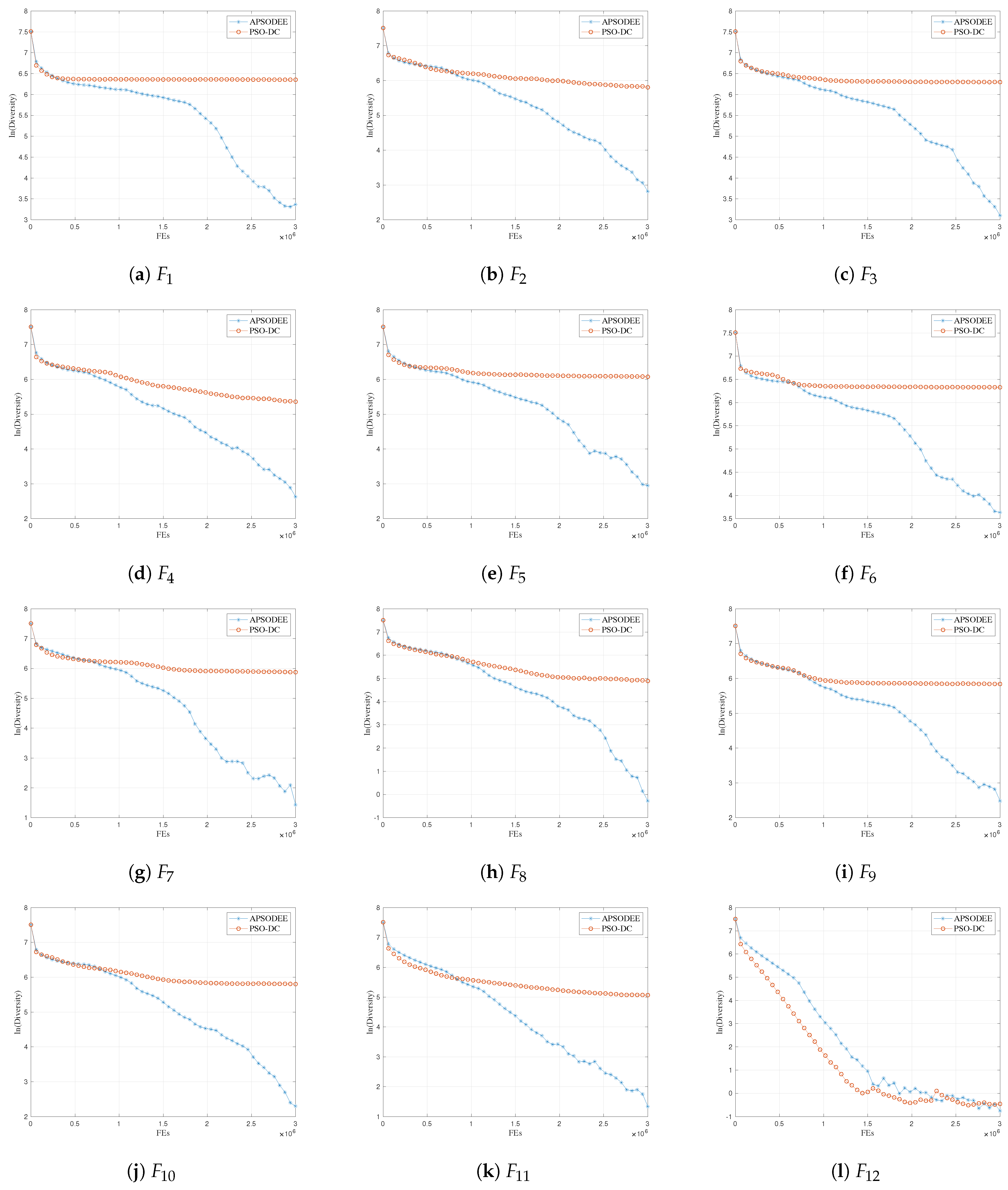
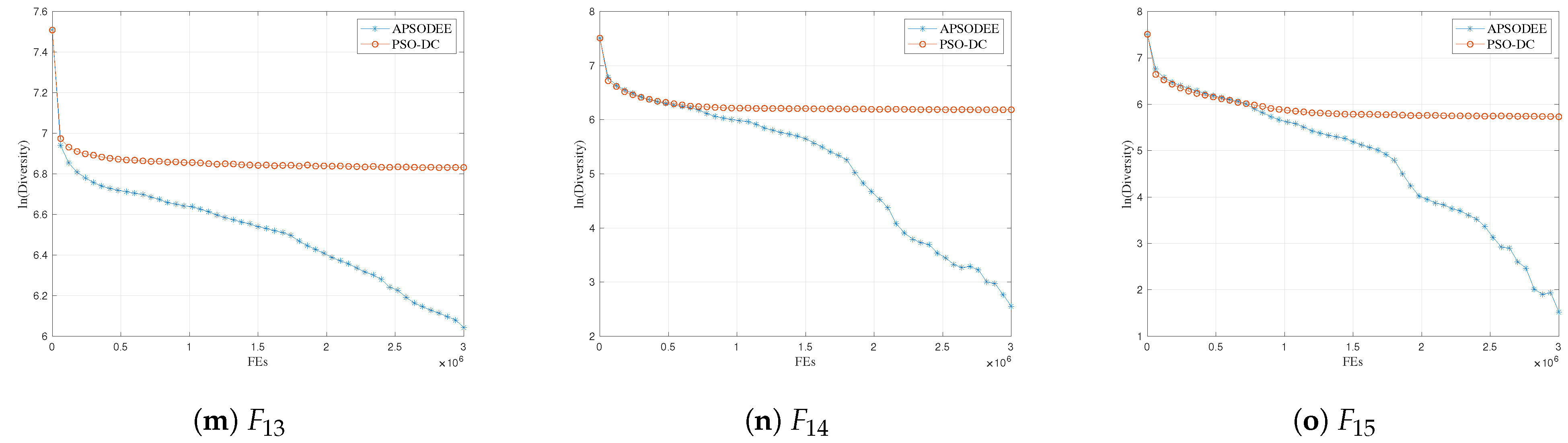
4.3. Diversity Preservation Characteristics

For the analysis of the diversity preservation characteristics of the proposed PSO-DC, this paper compares PSO-DC with APSO-DEE, which is a recently proposed PSO variant for LSOPs [1] based on the analysis method presented in [13].
In PSO-DC’s velocity update strategy, (2) can be rewritten as (12)–(14).
v i d ( t + 1 ) ω v i d ( t ) + θ 1 ( p 1 d ( t ) p i d ( t ) ) ,
θ 1 = r 1 + ϕ r 2 ,
p 1 d ( t ) = r 1 r 1 + ϕ r 2 e 1 d ( t ) + ϕ r 2 r 1 + ϕ r 2 e 2 d ( t ) .
Similarly, the velocity update strategy of APSO-DEE can be rewritten as (15)–(17):
v i d ( t + 1 ) ω v i d ( t ) + θ 2 ( p 2 d ( t ) p i d ( t ) ) ,
θ 2 = r 1 + ϕ r 2 ,
p 2 d ( t ) = r 1 r 1 + ϕ r 2 p c e , i d ( t ) + ϕ r 2 r 1 + ϕ r 2 p e d , i d ( t ) .
where p c e , i and p e d , i are exemplars in APSO-DEE for convergence and diversity, respectively.
Consequently, the exploration ability of PSO-DC and APSO-DEE is mainly influenced by the diversity of p 1 and p 2 . In APSO-DEE, p c e is the best particle of the sub-swarm that the i th particle is in, and it is shared by all the updated particles in this sub-swarm. In PSO-DC, e 1 and e 2 are both randomly selected with the proposed dual-competition strategy. Therefore, the diversity of p 1 should be better than that of p 2 . Furthermore, thanks to the dual-competition strategy, more than half of the particles can be preserved at each generation. In summary, the diversity preservation ability of PSO-DC is believed to be better than that of APSO-DEE, leading to a better exploration ability in PSO-DC.

5. Experimental Study

This section verifies the performance of the proposed algorithm: First, empirical comparisons are conducted to test PSO-DC by comparing it with seven peer algorithms. Second, the sensitivity analysis for the parameters is made to show the characteristics of PSO-DC. Finally, a comparison between PSO-DC and APSO-DEE on swarm diversity is presented to show the diversity preservation ability of the proposed algorithm.

5.1. Empirical Comparisons

5.1.1. Compared Algorithms and Benchmarks

To validate the performance of PSO-DC, seven popular algorithms for LSOPs were selected in the numerical comparisons, including DLLSO [13], APSO-DEE [1], TPLSO [39], RCI-PSO [18], DECC-DG2 [31], DECC-MDG [35], and MLSHADE-SPA [43]. Specifically, DLLSO, TPLSO, and RCI-PSO are three PSO variants building on different exemplar diversification strategies: APSO-DEE is designed with a decoupled learning structure, DECC-DG2 and DECC-MDG employ a CC framework, and MLSHADE-SPA is a recently proposed hybrid large-scale evolutionary algorithm.
In the comparisons, a recently proposed benchmark test suite [44] was adopted, where the benchmark functions were designed with heterogeneous modules based on 16 base functions, e.g., sphere function, elliptical function, Rosenbrock’s function, etc. Specifically, first, in comparison to the benchmarks posted in CEC 2010 [45] and CEC 2013 [44,46], benchmarks were designed by adopting a heterogeneous method to obtain differences between modules. Second, versatile coupled modules were designed, including three coupling topologies, and five types of coupling degrees (non-coupled, loosely coupled, moderately coupled, tightly coupled, and fully coupled) were introduced in the benchmarks. Therefore, the benchmarks in [44] should be more complicated. Detailed definitions of the benchmarks are presented in Appendix A, where Appendix A.1 presents the details of the base functions and Appendix A.2 defines the formulation of the benchmarks, respectively. Readers are referred to [44] for more details of the benchmarks.
All the algorithms were coded with Matlab 2022b and independently run 25 times on each benchmark on a computer with Windows 11 and an Intel I9 14900K.

5.1.2. Experimental Settings

For the experimental settings, the dimensionality of the benchmarks was set to 1000 and the maximum number of the fitness evaluations ( M a x F E s ) was adopted as the terminal criterion for the optimization process, which is set to 3 × 10 6 . For the parameter settings of the selected peer algorithms, the recommended settings in the corresponding references were adopted for fairness. For PSO-DC, according to the parameter sensitivity analysis, the swarm size N p o p and the parameter ϕ were set to 600 and 0.5, respectively. For the statistical analysis, the rank-sum test was adopted for the comparisons between PSO-DC and the peer algorithms, with the significance factor set to 0.05, and the Friedman test was utilized in the parameter analysis experiments.

5.1.3. Results

The numerical results are shown in Table 1, where the best average results on each benchmark are highlighted with gray background, and the symbols of “w/l/t” at the bottom of the table represent how many times that the performance of PSO-DC was significantly better, significantly worse, or tight in comparison to the corresponding results obtained by the peer algorithms. For the p values, the results are highlighted in bold if the performance of PSO-DC was significantly better than that of the peer algorithms.
From Table 1, one can find that the proposed PSO-DC is generally competitive with respect to the average performance: it outperforms the peer algorithms on 10 benchmarks out of the 15 test cases. To provide deeper insight, PSO-DC wins two, four, two, and two times on the loosely coupled functions F 2 to F 5 , moderately coupled functions F 6 to F 9 , tightly coupled functions F 10 to F 12 , and fully coupled functions F 13 to F 15 , respectively. Consequently, it is reasonable that PSO-DC has advantages in solving complicated benchmarks. Furthermore, for the comparison results of the statistical test, PSO significantly outperforms DLLSO, APSO-DEE, TPLSO, RCI-PSO, DECC-DG2, DECC-MDG, and MLSHADE-SPA for a total of 11, 11, 13, 10, 13, 13 and 12 times, respectively, which also demonstrates the competitiveness of PSO-DC. In summary, from the numerical comparison results, PSO-DC is competitive in solving LSOPs, especially for complicated benchmarks. This indicates that PSO-DC has been improved in balancing exploration and exploitation, benefiting from the improved diversity preservation ability.
Figure 2 presents the convergence curves of all the compared algorithms. One can find that PSO-DC shows moderate convergence speed, and the convergence of PSO-DC generally shows advantages during the latter optimization stage in comparison to the peer algorithms. A reasonable explanation for this funding is that PSO-DC is more promising in diversity preservation, which potentially first impacts its convergence speed while finally leading to better exploration of the search spaces.
In summary, the numerical comparison results above demonstrate the competitiveness of the proposed PSO-DC in solving LSOPs, indicating that PSO-DC enhances diversity preservation and thereby improves the balance between exploration and exploitation.

5.2. Parameter Sensitivity Analysis

In the parameter sensitivity analysis, experiments are conducted to investigate the influences of N p o p and ϕ on the performance of PSO-DC.

5.2.1. Analysis for N p o p

For the analysis of N p o p , ϕ is fixed to 0.5, and N p o p is set to 400, 500, 600, 800, and 1000 to show N p o p ’s influences on PSO-DC’s performance. The results are shown in Table 2. For the tests evaluating computational resource usage, the results are obtained with five independent runs. From Table 2, one can find that different swarm size settings lead to different performances, and PSO-DC performs relatively stable when N p o p 500 . This indicates that PSO-DC is able to provide good diversity and ensures exploration ability as long as the swarm size is not excessively small.

5.2.2. Analysis for ϕ

For the analysis of ϕ , N p o p is fixed to 500 and ϕ is varied from 0.1 to 0.6 with a step of 0.1. The results are shown in Table 3. One can find that ϕ = 0.5 evidently outperforms other settings, while PSO-DC is not sensitive to ϕ when ϕ 0.5 . This indicates that ϕ = 0.5 can help PSO-DC balance exploration and exploitation.

5.2.3. The Correlation between N p o p and ϕ

To further investigate the characteristics of PSO-DC, experiments are conducted to test the influences of different combinations of N p o p and ϕ on PSO-DC’s performance. The results are shown in Table 4 and Figure 3, which reconfirm the effectiveness of ϕ = 0.5 . Furthermore, one can find that excessively small or large combinations of N p o p and ϕ perform relative worse. A reasonable explanation is that excessively small combinations of swarm size and ϕ lead to poor swarm diversity resulting in poor exploration ability, while excessively large combinations of swarm size and ϕ make PSO-DC overly focused on diversity preservation, resulting in poor exploitation ability.

5.3. Diversity Comparison between PSO-DC and APSO-DEE

According to the discussion in Section 3 and Section 4.3, PSO-DC shows advantages in diversity preservation in comparison to APSO-DEE. To examine the theoretical analysis, this section presents a comparison between PSO-DC and APSO-DEE with respect to their swarm diversity trajectories in the whole optimization process. The swarm diversity is computed according to (18) and (19).
S t d ( P ) = 1 N i = 1 N d = 1 D ( p i d p ¯ i d ) 2 ,
p ¯ d = 1 N i = 1 N x i d .
The results are shown in Figure 4, experimentally proving that PSO-DC has better diversity preservation ability in comparison to APSO-DEE. This should benefit from the proposed dual-competition-based strategy. Considering that PSO-DC is also more promising in convergence speed than APSO-DEE according to the results in Figure 2, it can be concluded that the proposed strategy is capable of enhancing PSO-DC in balancing exploration and exploitation.

5.4. Scalability Test

In the scalability test experiment, the dimensionality of the benchmarks is set to 3000, and the parameter settings in Section 5.1.2 are adopted. To save time, each algorithm is run 10 times on each benchmark, and M a x F E s is also set to 3 × 10 6 . Note that F 12 and F 13 are not employed in this section, since their dimensionality cannot be changed according to the designs in [44]. DECCDG2 is not adopted in the scalability test. This is because DG2 is highly time-consuming when performing variable grouping when the dimensionality of the benchmarks is excessively large.
The results are shown in Table 5, where the average results of the compared algorithms are presented and the best average results are highlighted in bold. In general, PSO-DC outperforms all the peer algorithms on 12 benchmarks out of the 15 benchmarks with respect to the average results. The Friedman test results at the bottom of Table 5 also show the competitiveness of the proposed algorithm. It should be noted that PSO-DC shows promising results on the benchmarks with more complicated coupling characteristics, namely F 6 to F 11 and F 14 to F 15 (benchmarks with moderately, tightly, and fully coupled characteristics).

6. Conclusions and Future Work

Targeting the issue of diversity preservation in particle swarm optimization, this paper proposes a dual-competition-based strategy for particle swarm optimization to improve its diversity preservation ability in solving large-scale optimization problems. According to the theoretical and experimental results, the following two conclusions can be drawn: (i) The proposed algorithm is competitive when solving large-scale optimization problems. In particular, the proposed algorithm shows remarkable advantages over the peer algorithms when solving the complicated benchmarks. (ii) The proposed algorithm shows improved convergence speed and diversity, especially in the latter optimization stage. This indicates that the proposed dual-competition-based strategy is able to help improve the proposed algorithm in diversity preservation, thereby leading to enhanced performance in balancing exploration and exploitation.
However, the results show that the proposed algorithms still cannot effectively solve the benchmarks. Reasonable explanations could be that (i) the proposed algorithm cannot provide a sufficient search of the decision space due to limited computational resources or (ii) the solution update strategy of PSO inherently cannot efficiently conduct exploitation in huge search spaces. Consequently, in our future work, employing GPU devices and parallel computing methods to enhance the proposed algorithm’s computational efficiency and incorporating the proposed algorithm with specific local search techniques to enhance its exploitation ability can be promising research directions.

Author Contributions

Conceptualization, W.G. (Weijun Gao) and W.G. (Weian Guo); methodology, W.G. (Weian Guo) and X.P.; software, D.L.; validation, X.P. and W.G. (Weian Guo); formal analysis, W.G. (Weian Guo); investigation, D.L.; resources, X.P.; data curation, W.G. (Weijun Gao); writing—original draft preparation, W.G. (Weijun Gao); writing—review and editing, X.P.; visualization, W.G. (Weijun Gao); supervision, D.L.; project administration, X.P.; funding acquisition, W.G. (Weian Guo). All authors have read and agreed to the published version of the manuscript.

Funding

This work is supported by the National Natural Science Foundation of China under Grant Number 62273263, 72171172 and 71771176; Shanghai Municipal Science and Technology Major Project (2022-5-YB-09); Natural Science Foundation of Shanghai under Grant Number 23ZR1465400; The Study on the mechanism of industrial-education cocultivation for interdisciplinary technical and skilled personnel in Chinese intelligent manufacturing industry (Planning project for the 14th Five-Year Plan of National Education Sciences (BJA210093)).

Data Availability Statement

The data and code can be available on request by readers.

Conflicts of Interest

The authors declare no conflicts of interest.

Appendix A. Explanation of the Benchmarks Employed in the Experiment

In this section, the formulations of the benchmarks employed in Section 5 are presented. Note that the benchmarks are designed on the basis of the following base functions.

Appendix A.1. The Base Functions

  • Sphere Function
    f 1 ( x ) = i = 1 D x i 2 .
  • Elliptic Function
    f 2 ( x ) = i = 1 D 10 4 i 1 D 1 x i 2 .
  • Rotated Elliptic Function
    f 3 ( x ) = f 2 ( z ) ,
    z = R x .
  • Step Elliptic Function
    f 4 ( x ) = max z 1 10 6 , i = 2 D 10 4 i 1 D 1 z i 2 ,
    where z ^ = R x , and for i = 1 , , D , z i = 0.5 + z ^ i , if z ^ i > 0.5 0.5 + 10 z ^ i 10 , otherwise .
  • Rastrigin’s Function
    f 5 ( x ) = A i = 1 D z i 2 10 cos 2 π z i + 10 ,
    where z = 0.0512 x , A = 250 .
  • Buche–Rastrigin’s Function
    f 6 ( x ) = A i = 1 D ( z i 2 10 cos ( 2 π z i ) + 10 ) ,
    where A = 125 , f o r i = 1 , , D , z i = 0.0512 s i x i , s i = 10 × 10 1 2 i 1 D 1 , if x i > 0 and i is odd , 10 1 2 i 1 D 1 , otherwise . .
  • Griewank’s Function
    f 7 ( x ) = A 1 4000 i = 1 D z i 2 i = 1 D cos z i i + 1 ,
    where A = 10 4 , z = Λ 100 ( R x ) , Λ a is a D th dimensional diagonal matrix, and the diagonal element λ i i = α i 1 2 ( D 1 ) , for i = 1 , 2 , D .
  • Rotated Rastrigin’s Function
    f 8 ( x ) = f 5 ( z ) ,
    where z = Λ 10 T asy 0.2 ( T osz ( R ( 0.0512 x ) ) ) , T asy β : For i = 1 , 2 , , D , if x > 0 , x i = x i 1 + β i 1 D 1 x i , T osz : For i = 1 , 2 , , D , x i = sign ( x i ) exp ( x ^ i + 0.049 ( sin ( c 1 x ^ i ) + sin ( c 2 x ^ i ) ) ) , x ^ i = log ( | x i | ) , if x i 0 , otherwise x ^ i = 0 , sign ( · ) is a sign function, c 1 = 10 , if x i > 0 , otherwise, c 1 = 5.5 , and c 2 = 7.9 , if x i > 0 , otherwise c 2 = 3.1 .
  • Rotated Weierstrass Function
    f 9 ( x ) = i = 1 D k = 0 k max a k cos ( 2 π b k ( z i + 0.5 ) ) D k = 0 k max a k cos ( 2 π b k · 0.5 ) ,
    where z = R ( 0.005 x ) , a = 0.5 , b = 3 , k max = 20 , A = 10 4 .
  • Rotated Ackley’s Function
    f 10 ( x ) = a a exp b 1 D i = 1 D z i 2 exp 1 D i = 1 D cos ( 2 π z i ) + e ,
    where z = R ( 0.32 x ) , a = 3 × 10 4 , b = 0.5 .
  • Lunacek Bi-Rastrigin’s Function
    f 11 ( x ) = A min i = 1 D ( z i μ 0 ) 2 , d D + s i = 1 D ( z i μ 1 ) 2 + A i = 1 D ( 10 cos ( 2 π ( z i μ 0 ) ) + 10 ) ,
    where z = Λ 100 R ( 0.0512 x ) , A = 250 , μ 0 = 2.5 , μ 1 = ( μ 0 2 d ) / s , s = 1 1 / ( 2 D + 20 8.2 ) , d = 1 .
  • Modified Schwefel’s Function
    f 12 ( x ) = A 418.982887 D i = 1 D g ( z i ) ,
    where z i = y i + 420.9687462275036 , y = R ( 10 x ) , for i = 1 , , D , A = 30 , and
    g ( z i ) = z i sin ( | z i | ) , if | z i | 500 , ( 500 mod ( z i , 500 ) ) sin ( | 500 mod ( z i , 500 ) | ) ( z i 500 ) 2 10000 D , if z i > 500 , ( mod ( z i , 500 ) 500 ) sin ( | mod ( z i , 500 ) 500 | ) ( z i + 500 ) 2 10000 D , if z i < 500 .
  • Rosenbrock Function
    f 13 ( x ) = i = 1 D 1 100 ( z i 2 z i + 1 ) 2 + ( z i 1 ) 2 ,
    where z = 0.05 x + 1 .
  • Expanded Rosenbrock’s plus Grewangk’s Function
    f 14 ( x ) = A ( f 7 ( f 13 ( x 1 , x 2 ) ) + f 7 ( f 13 ( x 2 , x 3 ) ) + + f 7 ( f 13 ( x D 1 , x D ) ) + f 7 ( f 13 ( x D , x 1 ) ) ) ,
    where z = 0.05 x , A = 10 4 .
  • Expanded Schaffer’s Function
    f 15 ( x ) = A ( g ( z 1 , z 2 ) + g ( z 2 , z 3 ) + + g ( z D 1 , z D ) + g ( z D , z 1 ) ) ,
    where A = 4 × 10 4 , z = x + 1 , and g ( x , y ) = 0.5 + sin 2 ( x 2 + y 2 ) 0.5 ( 1 + 0.001 ( x 2 + y 2 ) ) 2 .
  • Composition Function
    f 16 ( x ) = w 1 · 10 f 8 ( x ) + w 2 · ( 10 3 f 10 ( x ) + 100 ) + w 3 · ( 2 f 12 ( x ) + 200 ) ,
    where f o r i = 1 , 2 , 3 , w i = 1 j = 1 D ( x j o i j ) 2 exp ( j = 1 D ( x j o i j ) 2 2 D σ i 2 ) , σ = [ 10 , 20 , 30 ] . Normalize the weights w i = w i / i = 1 3 w i , when x = o i , w j = 1 if j = i , otherwise w j = 0 .

Appendix A.2. The Benchmark Functions

With the aforementioned base functions, ref. [44] defines the benchmark functions as follows, where r is the coupling degree. More details can be found in [44]. Note that the meanings of r, S, ω , and ψ in the following are listed in Table A1. More detailed designs of the benchmarks can be found in [44].
Table A1. The description of ψ , S, ω , and r.
SymbolsDescriptions
ψ The set of base functions used to form the benchmark function.
SEach element in S denotes the size of the corresponding module in the benchmark function. Moreover, | S | represents the number of elements in the set S, which is the number of modules in the benchmark function.
rThe coupling degree of the benchmark function.
ω The weight for the modules of the benchmark function, which is adopted to generate imbalance of the modules.
  • F 1 : Partially Separable Function
    F 1 ( x ) = i = 1 | S | w i f b a s e i ( z i ) ,
    where
    • r = 0 % ;
    • Ψ = { f 13 , f 12 , f 1 , f 12 , f 3 , f 14 , f 3 , f 9 , f 7 , f 9 , f 7 , f 11 , f 4 , f 15 , f 1 , f 11 , f 7 , f 9 , f 3 , f 4 } ;
    • S = { 27 , 38 , 31 , 49 , 67 , 63 , 34 , 48 , 36 , 76 , 49 , 69 , 58 , 47 , 43 , 41 , 44 , 76 , 55 } ;
    • x [ 100 , 100 ] D ;
    • z = x o .
  • F 2 : Loosely Coupled Function 1 (Sequential Coupling Topology)
    F 2 ( x ) = i = 1 | S | w i f b a s e i ( z i ) ,
    where
    • r = 5 % ;
    • Ψ = { f 7 , f 1 , f 9 , f 7 , f 7 , f 11 , f 4 , f 10 , f 5 , f 12 , f 10 , f 9 , f 3 , f 9 , f 3 , f 13 , f 14 , f 8 , f 14 , f 4 } ;
    • S = { 30 , 71 , 73 , 63 , 51 , 35 , 62 , 79 , 37 , 61 , 40 , 30 , 43 , 59 , 51 , 60 , 51 , 53 , 48 , 53 } ;
    • x [ 100 , 100 ] D , b = { 1 , 0 , 0 , 0 , 1 , 0 , 0 , 0 , 1 , 1 , 1 , 0 , 0 , 0 , 0 , 0 , 0 , 1 , 0 , 0 } ;
    • z ( I c o n f o r a l l ) = x ( I c o n f o r a l l ) o ( I c o n f o r a l l ) ;
    • I c o n f o r a l l = i j | b ( j ) = 1 I i a l l ;
    • z i = x i o i , i { j | b ( j ) = 0 } .
  • F 3 : Loosely Coupled Function 2 (Randomly Coupling Topology)
    F 3 ( x ) = i = 1 | S | w i f b a s e i ( z i ) ,
    where
    • r = 5 % ;
    • Ψ = { f 9 , f 12 , f 12 , f 9 , f 15 , f 15 , f 3 , f 4 , f 14 , f 8 , f 1 , f 8 , f 11 , f 5 , f 11 , f 10 , f 12 , f 9 , f 16 , f 7 } ;
    • S = { 85 , 57 , 46 , 50 , 48 , 69 , 47 , 55 , 56 , 38 , 43 , 56 , 77 , 77 , 45 , 59 , 38 , 51 , 40 , 37 } ;
    • x [ 100 , 100 ] D ;
    • b = { 1 , 0 , 0 , 1 , 0 , 0 , 0 , 0 , 0 , 0 , 1 , 1 , 1 , 1 , 0 , 0 , 1 , 0 , 1 , 1 } ;
    • z ( I c o n f o r a l l ) = x ( I c o n f o r a l l ) o ( I c o n f o r a l l ) ;
    • I c o n f o r a l l = i j | b ( j ) = 1 I i a l l ;
    • z i = x i o i , i { j | b ( j ) = 0 } .
  • F 4 : Loosely Coupled Function 3 (Sequential Coupling Topology)
    F 4 ( x ) = i = 1 | S | w i f b a s e i ( z i ) ,
    where
    • r = 20 % ;
    • Ψ = { f 7 , f 9 , f 13 , f 12 , f 12 , f 4 , f 16 , f 1 , f 5 , f 7 , f 13 , f 4 , f 14 , f 16 , f 3 , f 10 , f 10 , f 7 , f 3 , f 16 } ;
    • S = { 22 , 94 , 57 , 24 , 109 , 78 , 51 , 104 , 25 , 70 , 33 , 67 , 118 , 28 , 150 , 22 , 21 , 24 , 37 , 66 } ;
    • x [ 100 , 100 ] D ;
    • b = { 1 , 0 , 0 , 0 , 0 , 1 , 0 , 1 , 1 , 1 , 0 , 1 , 0 , 0 , 0 , 1 , 0 , 1 , 1 , 0 } ;
    • z ( I c o n f o r a l l ) = x ( I c o n f o r a l l ) o ( I c o n f o r a l l ) ;
    • I c o n f o r a l l = i j | b ( j ) = 1 I i a l l ;
    • z i = x i o i , i { j | b ( j ) = 0 } .
  • F 5 : Loosely Coupled Function 4 (Random Coupling Topology)
    F 5 ( x ) = i = 1 | S | w i f b a s e i ( z i ) ,
    where
    • r = 20 % ;
    • Ψ = { f 4 , f 14 , f 4 , f 15 , f 8 , f 10 , f 13 , f 9 , f 5 , f 4 , f 13 , f 12 , f 8 , f 3 , f 15 , f 3 , f 7 , f 5 , f 11 , f 10 } ;
    • S = { 124 , 24 , 29 , 114 , 44 , 63 , 44 , 65 , 78 , 141 , 41 , 38 , 75 , 40 , 27 , 28 , 102 , 42 , 103 , 78 } ;
    • x [ 100 , 100 ] D ;
    • b = { 0 , 1 , 1 , 0 , 0 , 1 , 0 , 1 , 0 , 1 , 1 , 1 , 0 , 1 , 0 , 1 , 1 , 1 , 1 , 0 } ;
    • z ( I c o n f o r a l l ) = x ( I c o n f o r a l l ) o ( I c o n f o r a l l ) ;
    • I c o n f o r a l l = i j | b ( j ) = 1 I i a l l ;
    • z i = x i o i , i { j | b ( j ) = 0 } .
  • F 6 : Moderately Coupled Function 1 (Sequential Coupling Topology)
    F 6 ( x ) = i = 1 | S | w i f b a s e i ( z i ) ,
    where
    • r = 40 % ;
    • Ψ = { f 15 , f 12 , f 14 , f 1 , f 11 , f 10 , f 9 , f 7 , f 6 , f 10 , f 8 , f 12 , f 9 , f 10 , f 11 , f 16 , f 14 , f 7 , f 15 , f 14 } ;
    • S = { 50 , 60 , 84 , 50 , 83 , 96 , 47 , 112 , 41 , 221 , 46 , 72 , 74 , 55 , 53 , 49 , 53 , 51 , 66 , 37 } ;
    • x [ 100 , 100 ] D ;
    • b = { 1 , 1 , 1 , 1 , 0 , 0 , 1 , 0 , 1 , 0 , 1 , 0 , 0 , 0 , 1 , 1 , 0 , 1 , 1 , 1 } ;
    • z ( I c o n f o r a l l ) = x ( I c o n f o r a l l ) o ( I c o n f o r a l l ) ;
    • I c o n f o r a l l = i j | b ( j ) = 1 I i a l l ;
    • z i = x i o i , i { j | b ( j ) = 0 } .
  • F 7 : Moderately Coupled Function 2 (Random Coupling Topology)
    F 7 ( x ) = i = 1 | S | w i f b a s e i ( z i ) ,
    where
    • r = 40 % ;
    • Ψ = { f 10 , f 13 , f 8 , f 12 , f 16 , f 9 , f 9 , f 11 , f 5 , f 8 , f 11 , f 13 , f 7 , f 16 , f 5 , f 15 , f 4 , f 8 , f 15 , f 9 } ;
    • S = { 74 , 73 , 91 , 52 , 54 , 53 , 59 , 97 , 88 , 62 , 169 , 86 , 71 , 49 , 147 , 94 , 58 , 106 , 69 , 73 } ;
    • x [ 100 , 100 ] D ;
    • b = { 0 , 1 , 1 , 1 , 0 , 0 , 0 , 1 , 1 , 0 , 0 , 0 , 1 , 0 , 0 , 0 , 1 , 1 , 0 , 0 } ;
    • z ( I c o n f o r a l l ) = x ( I c o n f o r a l l ) o ( I c o n f o r a l l ) ;
    • I c o n f o r a l l = i j | b ( j ) = 1 I i a l l ;
    • z i = x i o i , i { j | b ( j ) = 0 } .
  • F 8 : Moderately Coupled Function 3 (Sequential Coupling Topology)
    F 8 ( x ) = i = 1 | S | w i f b a s e i ( z i ) ,
    where
    • r = 60 % ;
    • Ψ = { f 14 , f 16 , f 14 , f 2 , f 4 , f 1 , f 7 , f 7 , f 9 , f 8 , f 9 , f 9 , f 13 , f 12 , f 10 , f 7 , f 13 , f 16 , f 14 , f 4 } ;
    • S = { 94 , 110 , 65 , 108 , 72 , 61 , 74 , 83 , 77 , 89 , 75 , 63 , 54 , 77 , 66 , 101 , 74 , 92 , 79 , 86 } ;
    • x [ 100 , 100 ] D ;
    • b = { 1 , 1 , 0 , 1 , 1 , 1 , 0 , 1 , 0 , 0 , 1 , 0 , 0 , 1 , 1 , 1 , 1 , 0 , 1 , 1 } ;
    • z ( I c o n f o r a l l ) = x ( I c o n f o r a l l ) o ( I c o n f o r a l l ) ;
    • I c o n f o r a l l = i j | b ( j ) = 1 I i a l l ;
    • z i = x i o i , i { j | b ( j ) = 0 } .
  • F 9 : Moderately Coupled Function 4 (Random Coupling Topology)
    F 9 ( x ) = i = 1 | S | w i f b a s e i ( z i ) ,
    where
    • r = 60 % ;
    • Ψ = { f 12 , f 9 , f 8 , f 3 , f 3 , f 4 , f 7 , f 4 , f 2 , f 6 , f 3 , f 15 , f 16 , f 4 , f 12 , f 10 , f 15 , f 11 , f 9 , f 12 } ;
    • S = { 76 , 81 , 81 , 102 , 102 , 79 , 91 , 98 , 86 , 106 , 83 , 90 , 106 , 92 , 95 , 112 , 152 , 80 , 126 , 87 } ;
    • x [ 100 , 100 ] D ;
    • b = { 1 , 1 , 0 , 0 , 0 , 0 , 1 , 0 , 1 , 0 , 1 , 1 , 1 , 0 , 0 , 1 , 1 , 1 , 0 , 0 } ;
    • z ( I c o n f o r a l l ) = x ( I c o n f o r a l l ) o ( I c o n f o r a l l ) ;
    • I c o n f o r a l l = i j | b ( j ) = 1 I i a l l ;
    • z i = x i o i , i { j | b ( j ) = 0 } .
  • F 10 : Tightly Coupled Function 1 (Sequential Coupling Topology)
    F 10 ( x ) = i = 1 | S | w i f b a s e i ( z i ) ,
    where
    • r = 80 % ;
    • Ψ = { f 13 , f 1 , f 11 , f 12 , f 8 , f 4 , f 4 , f 13 , f 3 , f 2 , f 11 , f 16 , f 7 , f 9 , f 14 , f 10 , f 12 , f 11 , f 15 , f 12 } ;
    • S = { 89 , 113 , 77 , 84 , 81 , 84 , 87 , 91 , 86 , 82 , 92 , 90 , 80 , 102 , 95 , 81 , 99 , 95 , 120 , 73 } ;
    • x [ 100 , 100 ] D ;
    • b = { 1 , 1 , 1 , 1 , 1 , 1 , 1 , 0 , 1 , 0 , 0 , 0 , 1 , 0 , 0 , 0 , 0 , 1 , 0 , 1 } ;
    • z ( I c o n f o r a l l ) = x ( I c o n f o r a l l ) o ( I c o n f o r a l l ) ;
    • I c o n f o r a l l = i j | b ( j ) = 1 I i a l l ;
    • z i = x i o i , i { j | b ( j ) = 0 } .
  • F 11 : Tightly Coupled Function 2 (Sequential Coupling Topology)
    F 11 ( x ) = i = 1 | S | w i f b a s e i ( z i ) ,
    where
    • r = 80 % ;
    • Ψ = { f 3 , f 16 , f 8 , f 12 , f 7 , f 8 , f 9 , f 8 , f 16 , f 14 , f 12 , f 10 , f 15 , f 14 , f 3 , f 11 , f 1 , f 2 , f 16 , f 3 } ;
    • S = { 97 , 115 , 123 , 93 , 138 , 100 , 113 , 99 , 118 , 118 , 90 , 98 , 127 , 113 , 101 , 108 , 108 , 106 , 118 , 148 } ;
    • x [ 100 , 100 ] D ;
    • b = { 0 , 1 , 1 , 1 , 1 , 0 , 0 , 0 , 0 , 0 , 1 , 1 , 1 , 1 , 0 , 0 , 0 , 1 , 0 , 1 } ;
    • z ( I c o n f o r a l l ) = x ( I c o n f o r a l l ) o ( I c o n f o r a l l ) ;
    • I c o n f o r a l l = i j | b ( j ) = 1 I i a l l ;
    • z i = x i o i , i { j | b ( j ) = 0 } .
  • F 12 : Tightly Coupled Function 3 (Sequential Coupling Topology)
    F 12 ( x ) = f 13 ( z ) ,
    where
    • r = ( D 2 ) / D ;
    • x [ 100 , 100 ] D ;
    • z = x o .
  • F 13 : Fully Coupled Function 1 (Ring Coupling Topology)
    F 13 ( x ) = f 15 ( z ) ,
    where
    • r = 100 % ;
    • x [ 100 , 100 ] D ;
    • z = x o .
  • F 14 : Fully Coupled Function 2 (Ring Coupling Topology)
    F 14 ( x ) = i = 1 | S | w i f b a s e i ( z i ) ,
    where
    • r = 100 % ;
    • Ψ = { f 14 , f 7 , f 14 , f 1 , f 14 , f 16 , f 9 , f 4 , f 9 , f 4 , f 13 , f 6 , f 9 , f 15 , f 11 , f 4 , f 15 , f 15 , f 13 , f 13 } ;
    • S = { 88 , 104 , 106 , 96 , 94 , 96 , 110 , 96 , 88 , 106 , 105 , 93 , 103 , 105 , 98 , 96 , 103 , 105 , 105 , 103 } ;
    • x [ 100 , 100 ] D ;
    • b = { 0 , 0 , 0 , 1 , 0 , 1 , 0 , 0 , 1 , 1 , 1 , 0 , 1 , 1 , 1 , 0 , 1 , 0 , 0 , 0 } ;
    • z ( I c o n f o r a l l ) = x ( I c o n f o r a l l ) o ( I c o n f o r a l l ) ;
    • I c o n f o r a l l = i j | b ( j ) = 1 I i a l l ;
    • z i = x i o i , i { j | b ( j ) = 0 } .
  • F 15 : Fully Coupled Function 3 (Random Coupling Topology)
    F 15 ( x ) = i = 1 | S | w i f b a s e i ( z i ) ,
    where
    • r = 100 % ;
    • Ψ = { f 14 , f 3 , f 15 , f 12 , f 16 , f 9 , f 5 , f 3 , f 2 , f 4 , f 15 , f 13 , f 12 , f 14 , f 13 , f 4 , f 3 , f 9 , f 12 , f 4 } ;
    • S = { 117 , 117 , 121 , 118 , 126 , 132 , 119 , 102 , 132 , 130 , 126 , 125 , 135 , 124 , 141 , 104 , 139 , 117 , 135 , 119 } ;
    • x [ 100 , 100 ] D ;
    • b = { 1 , 0 , 1 , 1 , 0 , 0 , 1 , 0 , 0 , 0 , 1 , 1 , 1 , 0 , 1 , 0 , 1 , 1 , 1 , 1 } ;
    • z ( I c o n f o r a l l ) = x ( I c o n f o r a l l ) o ( I c o n f o r a l l ) ;
    • I c o n f o r a l l = i j | b ( j ) = 1 I i a l l ;
    • z i = x i o i , i { j | b ( j ) = 0 } .

References

  1. Li, D.; Guo, W.; Lerch, A.; Li, Y.; Wang, L.; Wu, Q. An adaptive particle swarm optimizer with decoupled exploration and exploitation for large scale optimization. Swarm Evol. Comput. 2021, 10, 100789. [Google Scholar] [CrossRef]
  2. Liu, Y.; Xing, T.; Zhou, Y.; Li, N.; Ma, L.; Wen, Y.; Liu, C.; Shi, H. A large-scale multi-objective brain storm optimization algorithm based on direction vectors and variance analysis. In Proceedings of the International Conference on Swarm Intelligence, Qingdao, China, 17–21 July 2023; Springer: Berlin/Heidelberg, Germany, 2023; pp. 413–424. [Google Scholar]
  3. Ma, L. Evolutionary computation-based machine learning and its applications for multi-robot systems. Front. Neuro-Robot. 2023, 17, 1177909. [Google Scholar] [CrossRef] [PubMed]
  4. Li, J.; Cheng, S. Parameter settings in particle swarm optimization algorithms: A survey. Int. J. Autom. Control. 2022, 16, 164–182. [Google Scholar] [CrossRef]
  5. Chaturvedi, S.; Kumar, N.; Kumar, R.A. PSO-optimized novel PID neural network model for temperature control of jacketed CSTR: Design, simulation, and a comparative study. Soft Comput. 2024, 28, 4759–4773. [Google Scholar] [CrossRef]
  6. Karakuzu, C.; Karakaya, F.; Cavuslu, M.A. FPGA implementation of neuro-fuzzy system with improved PSO learning. Neural Netw. 2016, 79, 128–140. [Google Scholar] [CrossRef] [PubMed]
  7. Sivanandam, S.N.; Deepa, S.N. Genetic Algorithms; Springer: Berlin/Heidelberg, Germany, 2008. [Google Scholar]
  8. Dorigo, M.; Birattari, M.; Stutzle, T. Ant colony optimization. IEEE Comput. Intell. Mag. 2006, 1, 28–39. [Google Scholar] [CrossRef]
  9. Chaturvedi, S.; Kumar, N.; Kumar, R. Two Feedback PID Controllers Tuned with Teaching-Learning-Based Optimization Algorithm for Ball and Beam System. IETE J. Res. 2023, 5, 1–10. [Google Scholar] [CrossRef]
  10. Cheng, S.; Qin, Q.; Chen, J.; Shi, Y. Brain storm optimization algorithm: A review. Artif. Intell. Rev. 2016, 46, 445–458. [Google Scholar] [CrossRef]
  11. Shami, T.M.; El-Saleh, A.A.; Alswaitti, M.; Al-Tashi, Q.; Summakieh, M.A.; Mirjalili, S. Particle swarm optimization: A comprehensive survey. IEEE Access 2022, 10, 10031–10061. [Google Scholar] [CrossRef]
  12. Cheng, R.; Jin, Y. A competitive swarm optimizer for large scale optimization. IEEE Trans. Cybern. 2014, 45, 191–204. [Google Scholar] [CrossRef]
  13. Yang, Q.; Chen, W.; Da, D.; Li, Y.; Gu, T.; Zhang, J. A level-based learning swarm optimizer for large-scale optimization. IEEE Trans. Evol. Comput. 2017, 22, 578–594. [Google Scholar] [CrossRef]
  14. Cheng, R.; Jin, Y. A social learning particle swarm optimization algorithm for scalable optimization. Inf. Sci. 2015, 291, 43–60. [Google Scholar] [CrossRef]
  15. Yang, Q.; Chen, W.; Gu, T.; Jin, H.; Mao, W.; Zhang, J. An adaptive stochastic dominant learning swarm optimizer for high-dimensional optimization. IEEE Trans. Cybern. 2020, 52, 1960–1976. [Google Scholar] [CrossRef] [PubMed]
  16. Song, G.; Yang, Q.; Gao, X.; Ma, Y.; Lu, Z.; Zhang, J. An adaptive level-based learning swarm optimizer for large-scale optimization. In Proceedings of the 2021 IEEE International Conference on Systems, Man, and Cybernetics, Melbourne, Australia, 17 October 2021; pp. 152–159. [Google Scholar]
  17. Yang, Q.; Song, G.; Gao, X.; Lu, Z.; Jeon, S.; Zhang, J. A random elite ensemble learning swarm optimizer for high-dimensional optimization. Complex Intell. Syst. 2023, 9, 5467–5500. [Google Scholar] [CrossRef]
  18. Yang, Q.; Song, G.; Chen, W.; Jia, Y.; Gao, X.; Lu, Z.; Jeon, S.W.; Zhang, J. Random contrastive interaction for particle swarm optimization in high-dimensional environment. IEEE Trans. Evol. Comput. 2023. [Google Scholar] [CrossRef]
  19. Wang, Z.; Yang, Q.; Zhang, Y.; Chen, S.; Wang, Y. Superiority combination learning distributed particle swarm optimization for large-scale optimization. Appl. Soft Comput. 2023, 136, 110101. [Google Scholar] [CrossRef]
  20. Li, D.; Guo, W.; Wang, L.; Wu, Q. A modified apsodee for large scale optimization. In Proceedings of the 2021 IEEE Congress on Evolutionary Computation (CEC), Krakow, Poland, 28 June–1 July 2021; pp. 1976–1982. [Google Scholar]
  21. Li, D.; Wang, L.; Guo, W.; Zhang, M.; Hu, B.; Wu, Q. A particle swarm optimizer with dynamic balance of convergence and diversity for large-scale optimization. Appl. Soft Comput. 2023, 132, 109852. [Google Scholar] [CrossRef]
  22. Jia, D.; Zheng, G.; Qu, B.; Khan, M.K. A hybrid particle swarm optimization algorithm for high-dimensional problems. Comput. Ind. Eng. 2011, 61, 1117–1122. [Google Scholar] [CrossRef]
  23. Tang, D.; Cai, Y.; Zhao, J.; Xue, Y. A quantum-behaved particle swarm optimization with memetic algorithm and memory for continuous non-linear large scale problems. Inf. Sci. 2014, 289, 162–189. [Google Scholar] [CrossRef]
  24. Tao, M.; Huang, S.; Li, Y.; Yan, M.; Zhou, Y. SA-PSO based optimizing reader deployment in large-scale RFID Systems. J. Netw. Comput. Appl. 2015, 52, 90–100. [Google Scholar] [CrossRef]
  25. Ali, A.F.; Tawhid, M.A. A hybrid particle swarm optimization and genetic algorithm with population partitioning for large scale optimization problems. Ain Shams Eng. J. 2017, 8, 191–206. [Google Scholar] [CrossRef]
  26. Van, D.B.F.; Engelbrecht, A.P. A cooperative approach to particle swarm optimization. IEEE Trans. Evol. Comput. 2004, 8, 225–239. [Google Scholar]
  27. Li, X.; Yao, X. Tackling high dimensional nonseparable optimization problems by cooperatively coevolving particle swarms. In Proceedings of the 2009 IEEE Congress on Evolutionary Computation, Trondheim, Norway, 18–21 May 2009; pp. 1546–1553. [Google Scholar]
  28. Li, X.; Yao, X. Cooperatively coevolving particle swarms for large scale optimization. IEEE Trans. Evol. Comput. 2011, 16, 210–224. [Google Scholar]
  29. Chen, K.; Xue, B.; Zhang, M.; Zhou, F. Novel chaotic grouping particle swarm optimization with a dynamic regrouping strategy for solving numerical optimization tasks. Knowl. Based Syst. 2020, 194, 105568. [Google Scholar] [CrossRef]
  30. Omidvar, M.N.; Li, X.; Mei, Y.; Yao, X. Cooperative co-evolution with differential grouping for large scale optimization. IEEE Trans. Evol. Comput. 2013, 18, 378–393. [Google Scholar] [CrossRef]
  31. Omidvar, M.N.; Yang, M.; Mei, Y.; Li, X.; Yao, X. DG2: A faster and more accurate differential grouping for large-scale black-box optimization. IEEE Trans. Evol. Comput. 2017, 21, 929–942. [Google Scholar] [CrossRef]
  32. Sun, Y.; Kirley, M.; Halgamuge, S.K. A recursive decomposition method for large scale continuous optimization. IEEE Trans. Evol. Comput. 2017, 22, 647–661. [Google Scholar] [CrossRef]
  33. Sun, Y.; Omidvar, M.N.; Kirley, M.; Li, X. Adaptive threshold parameter estimation with recursive differential grouping for problem decomposition. In Proceedings of the Genetic and Evolutionary Computation Conference, Kyoto, Japan, 15–19 July 2018; pp. 889–896. [Google Scholar]
  34. Yang, M.; Zhou, A.; Li, C.; Yao, X. An efficient recursive differential grouping for large-scale continuous problems. IEEE Trans. Evol. Comput. 2020, 25, 159–171. [Google Scholar] [CrossRef]
  35. Ma, X.; Huang, Z.; Li, X.; Wang, L.; Qi, Y.; Zhu, Z. Merged differential grouping for large-scale global optimization. IEEE Trans. Evol. Comput. 2022, 26, 1439–1451. [Google Scholar] [CrossRef]
  36. Cao, B.; Gu, Y.; Lv, Z.; Yang, S.; Zhao, J.; Li, Y. RFID reader anticollision based on distributed parallel particle swarm optimization. IEEE Internet Things J. 2020, 8, 3099–3107. [Google Scholar] [CrossRef]
  37. Liu, X.; Zhan, Z.; Zhang, J. Incremental particle swarm optimization for large-scale dynamic optimization with changing variable interactions. Appl. Soft Comput. 2023, 141, 110320. [Google Scholar] [CrossRef]
  38. Wang, F.; Wang, X.; Sun, S. A reinforcement learning level-based particle swarm optimization algorithm for large-scale optimization. Inf. Sci. 2022, 602, 298–312. [Google Scholar] [CrossRef]
  39. Lan, R.; Zhu, Y.; Lu, H.; Liu, Z.; Luo, X. A two-phase learning-based swarm optimizer for large-scale optimization. IEEE Trans. Cybern. 2020, 51, 6284–6293. [Google Scholar] [CrossRef] [PubMed]
  40. Zhang, E.; Nie, Z.; Yang, Q.; Wang, Y.; Liu, D.; Jeon, S.W.; Zhang, J. Heterogeneous cognitive learning particle swarm optimization for large-scale optimization problems. Inf. Sci. 2023, 633, 321–342. [Google Scholar] [CrossRef]
  41. Bonyadi, M.R.; Michalewicz, Z. Stability analysis of the particle swarm optimization without stagnation assumption. IEEE Trans. Evol. Comput. 2015, 20, 814–819. [Google Scholar] [CrossRef]
  42. Zhang, H. A discrete-time switched linear model of the particle swarm optimization algorithm. Swarm Evol. Comput. 2020, 52, 100606. [Google Scholar] [CrossRef]
  43. Hadi, A.A.; Mohamed, A.W.; Jambi, K.M. LSHADE-SPA memetic framework for solving large-scale optimization problems. Complex Intell. Syst. 2019, 5, 25–40. [Google Scholar] [CrossRef]
  44. Xu, P.; Luo, W.; Lin, X.; Zhang, J.; Wang, X. A large-scale continuous optimization benchmark suite with versatile coupled heterogeneous modules. Swarm Evol. Comput. 2023, 78, 101280. [Google Scholar] [CrossRef]
  45. Tang, K.; Li, X.; Suganthan, P.N.; Yang, Z.; Thomas, W. Benchmark Functions for the CEC 2010 Special Session and Competition on Large-Scale Global Optimization; Nature Inspired Computation and Applications Laboratory, USTC: Hefei, China, 2007; Volume 24, pp. 1–18. [Google Scholar]
  46. Li, X.; Tang, K.; Omidvar, M.N.; Yang, Z.; Qin, K. Benchmark functions for the CEC 2013 special session and competition on large-scale global optimization. Gene 2013, 7, 8. [Google Scholar]
Figure 1. Sketch of the proposed exemplars and updated particles selection mechanism.
Mathematics 12 01738 g001
Figure 2. The convergence curves of the compared algorithms.
Mathematics 12 01738 g002aMathematics 12 01738 g002b
Figure 3. The heatmap of the results in Table 4.
Mathematics 12 01738 g003
Figure 4. The swarm diversity curves of the compared algorithms.
Mathematics 12 01738 g004aMathematics 12 01738 g004b
Table 1. The numerical results of the algorithms with benchmark dimensionality of 1000 and M a x F E s = 3 × 10 6 .
FunctionQualityDLLSOAPSODEETPLSORCIPSODECCDG2DECCMDGMLSHADESPAPSO-DC
F 1 Mean5.47 × 10 7 6.42 × 10 7 2.00 × 10 8 7.48 × 10 7 6.00 × 10 7 1.53 × 10 8 6.28 × 10 7 2.09 × 10 8
Std1.34 × 10 7 1.51 × 10 7 2.37 × 10 7 1.43 × 10 7 5.95 × 10 6 3.92 × 10 6 6.51 × 10 6 5.39 × 10 6
p-value1.42 × 10 9 1.42 × 10 9 2.57 × 10 2 1.42 × 10 9 1.38 × 10 9 1.42 × 10 9 1.41 × 10 9 -
F 2 Mean2.45 × 10 8 1.87 × 10 8 2.89 × 10 8 2.09 × 10 8 5.99 × 10 8 3.91 × 10 8 2.96 × 10 8 1.38 × 10 8
Std6.09 × 10 7 4.63 × 10 7 4.30 × 10 7 4.65 × 10 7 1.18 × 10 8 9.62 × 10 7 6.94 × 10 7 1.29 × 10 7
p-value1.42 × 10 9 1.80 × 10 9 1.42 × 10 9 1.42 × 10 9 1.38 × 10 9 1.42 × 10 9 1.42 × 10 9 -
F 3 Mean4.73 × 10 7 4.37 × 10 7 7.51 × 10 7 5.01 × 10 7 3.82 × 10 8 1.33 × 10 8 1.83 × 10 8 7.14 × 10 7
Std4.11 × 10 6 4.42 × 10 6 7.04 × 10 6 3.73 × 10 6 1.39 × 10 8 1.60 × 10 7 1.74 × 10 8 4.20 × 10 6
p-value1.42 × 10 9 1.42 × 10 9 1.28 × 10 3 1.42 × 10 9 1.38 × 10 9 1.42 × 10 9 9.29 × 10 9 -
F 4 Mean7.99 × 10 7 5.78 × 10 7 8.89 × 10 7 6.83 × 10 7 2.90 × 10 8 2.80 × 10 8 1.92 × 10 8 3.53 × 10 7
Std1.80 × 10 7 1.50 × 10 7 2.79 × 10 7 1.58 × 10 7 4.99 × 10 7 6.63 × 10 7 2.64 × 10 7 1.10 × 10 7
p-value1.42 × 10 9 1.84 × 10 8 1.80 × 10 9 1.60 × 10 9 1.38 × 10 9 1.42 × 10 9 1.42 × 10 9 -
F 5 Mean3.24 × 10 7 3.23 × 10 7 3.58 × 10 7 3.72 × 10 7 6.85 × 10 7 1.06 × 10 8 6.61 × 10 7 4.67 × 10 7
Std3.00 × 10 6 2.14 × 10 6 3.37 × 10 6 2.89 × 10 6 7.43 × 10 6 1.51 × 10 7 8.75 × 10 6 5.01 × 10 6
p-value1.42 × 10 9 1.42 × 10 9 2.03 × 10 9 1.80 × 10 9 1.38 × 10 9 1.42 × 10 9 1.42 × 10 9 -
F 6 Mean1.73 × 10 8 1.44 × 10 8 1.67 × 10 8 1.40 × 10 8 1.20 × 10 9 4.92 × 10 8 2.90 × 10 8 1.24 × 10 8
Std5.68 × 10 7 5.13 × 10 7 4.92 × 10 7 3.84 × 10 7 1.40 × 10 8 6.83 × 10 7 8.30 × 10 7 5.71 × 10 7
p-value6.96 × 10 5 3.28 × 10 2 1.81 × 10 4 4.16 × 10 2 1.38 × 10 9 1.42 × 10 9 1.80 × 10 9 -
F 7 Mean1.29 × 10 8 1.14 × 10 8 1.21 × 10 8 1.25 × 10 8 2.92 × 10 8 2.37 × 10 8 1.39 × 10 8 9.41 × 10 7
Std2.44 × 10 7 1.37 × 10 7 2.52 × 10 7 1.37 × 10 7 3.90 × 10 7 3.85 × 10 7 1.41 × 10 7 1.06 × 10 7
p-value1.60 × 10 9 5.85 × 10 9 3.21 × 10 8 1.60 × 10 9 1.38 × 10 9 1.42 × 10 9 1.42 × 10 9 -
F 8 Mean1.46 × 10 8 1.31 × 10 8 1.48 × 10 8 1.41 × 10 8 1.59 × 10 8 1.89 × 10 8 1.91 × 10 8 1.26 × 10 8
Std2.93 × 10 6 1.86 × 10 6 4.79 × 10 6 2.93 × 10 6 4.02 × 10 6 1.15 × 10 7 9.75 × 10 6 2.22 × 10 6
p-value1.42 × 10 9 1.60 × 10 9 1.42 × 10 9 1.42 × 10 9 1.38 × 10 9 1.42 × 10 9 1.42 × 10 9 -
F 9 Mean6.48 × 10 8 5.24 × 10 8 6.71 × 10 8 6.10 × 10 8 1.13 × 10 9 1.33 × 10 9 1.03 × 10 9 4.53 × 10 8
Std5.37 × 10 7 2.26 × 10 7 8.27 × 10 7 4.45 × 10 7 1.37 × 10 8 1.27 × 10 8 8.67 × 10 7 2.03 × 10 7
p-value1.42 × 10 9 1.42 × 10 9 1.42 × 10 9 1.42 × 10 9 1.38 × 10 9 1.42 × 10 9 1.42 × 10 9 -
F 10 Mean4.72 × 10 8 3.76 × 10 8 4.31 × 10 8 4.35 × 10 8 9.29 × 10 8 6.62 × 10 8 7.07 × 10 8 3.13 × 10 8
Std4.87 × 10 7 4.78 × 10 7 4.69 × 10 7 5.60 × 10 7 2.11 × 10 8 1.51 × 10 8 7.67 × 10 7 1.45 × 10 7
p-value1.42 × 10 9 2.57 × 10 9 1.42 × 10 9 1.42 × 10 9 1.38 × 10 9 1.42 × 10 9 1.42 × 10 9 -
F 11 Mean1.66 × 10 8 1.54 × 10 8 1.67 × 10 8 1.61 × 10 8 1.79 × 10 8 2.13 × 10 8 1.90 × 10 8 1.52 × 10 8
Std3.22 × 10 6 1.41 × 10 6 2.79 × 10 6 2.72 × 10 6 6.50 × 10 6 6.40 × 10 6 5.94 × 10 6 1.26 × 10 6
p-value1.42 × 10 9 2.57 × 10 9 1.42 × 10 9 1.42 × 10 9 1.38 × 10 9 1.42 × 10 9 1.42 × 10 9 -
F 12 Mean1.70 × 10 3 1.16 × 10 3 1.91 × 10 3 1.49 × 10 3 1.63 × 10 3 2.94 × 10 3 5.50 × 10 2 1.00 × 10 3
Std2.10 × 10 2 1.13 × 10 2 1.94 × 10 2 1.55 × 10 2 2.44 × 10 2 2.31 × 10 2 1.86 × 10 2 4.75 × 10 1
p-value1.42 × 10 9 2.29 × 10 9 1.42 × 10 9 1.42 × 10 9 1.38 × 10 9 1.42 × 10 9 1.42 × 10 9 -
F 13 Mean1.94 × 10 7 1.94 × 10 7 1.95 × 10 7 1.91 × 10 7 6.63 × 10 5 1.93 × 10 7 1.88 × 10 6 1.95 × 10 7
Std5.08 × 10 4 5.56 × 10 4 4.51 × 10 4 7.82 × 10 5 5.98 × 10 4 4.29 × 10 4 2.43 × 10 5 3.91 × 10 4
p-value2.98 × 10 2 2.05 × 10 8 6.57 × 10 9 1.42 × 10 9 1.38 × 10 9 1.42 × 10 9 1.42 × 10 9 -
F 14 Mean4.23 × 10 8 3.37 × 10 8 4.37 × 10 8 3.81 × 10 8 1.46 × 10 9 8.46 × 10 8 7.80 × 10 8 2.75 × 10 8
Std4.53 × 10 7 3.69 × 10 7 6.53 × 10 7 3.71 × 10 7 1.26 × 10 8 6.48 × 10 7 6.57 × 10 7 3.64 × 10 7
p-value1.42 × 10 9 4.64 × 10 9 1.42 × 10 9 1.42 × 10 9 1.38 × 10 9 1.42 × 10 9 1.42 × 10 9 -
F 15 Mean7.11 × 10 8 5.92 × 10 8 6.99 × 10 8 6.88 × 10 8 1.10 × 10 9 1.49 × 10 9 1.15 × 10 9 5.68 × 10 8
Std4.40 × 10 7 2.42 × 10 7 3.10 × 10 7 4.30 × 10 7 8.45 × 10 7 1.21 × 10 8 7.14 × 10 7 2.63 × 10 7
p-value1.42 × 10 9 1.51 × 10 5 1.42 × 10 9 1.42 × 10 9 1.38 × 10 9 1.42 × 10 9 1.42 × 10 9 -
w/l/t11/4/011/4/013/2/010/5/013/2/013/2/012/3/0-
Table 2. The performance of PSO-DC obtained with different settings of N p o p .
Function Npop = 400 Npop = 500 Npop = 600 Npop = 800 Npop = 1000
F 1 2.08 × 10 8 2.08 × 10 8 2.09 × 10 8 2.11 × 10 8 2.13 × 10 8
F 2 1.69 × 10 8 1.49 × 10 8 1.39 × 10 8 1.33 × 10 8 1.30 × 10 8
F 3 7.81 × 10 7 7.38 × 10 7 7.21 × 10 7 7.21 × 10 7 7.47 × 10 7
F 4 4.62 × 10 7 4.00 × 10 7 3.45 × 10 7 3.00 × 10 7 3.25 × 10 7
F 5 3.91 × 10 7 4.28 × 10 7 4.71 × 10 7 4.99 × 10 7 5.21 × 10 7
F 6 1.51 × 10 8 1.28 × 10 8 1.23 × 10 8 1.21 × 10 8 1.10 × 10 8
F 7 1.04 × 10 8 9.73 × 10 7 9.28 × 10 7 8.72 × 10 7 9.54 × 10 7
F 8 1.30 × 10 8 1.27 × 10 8 1.26 × 10 8 1.24 × 10 8 1.25 × 10 8
F 9 5.35 × 10 8 4.78 × 10 8 4.53 × 10 8 4.31 × 10 8 4.26 × 10 8
F 10 3.20 × 10 8 3.22 × 10 8 3.12 × 10 8 3.02 × 10 8 3.07 × 10 8
F 11 1.54 × 10 8 1.53 × 10 8 1.52 × 10 8 1.52 × 10 8 1.53 × 10 8
F 12 1.13 × 10 3 1.02 × 10 3 1.01 × 10 3 9.94 × 10 2 9.92 × 10 2
F 13 1.95 × 10 7 1.95 × 10 7 1.95 × 10 7 1.95 × 10 7 1.95 × 10 7
F 14 2.88 × 10 8 2.85 × 10 8 2.78 × 10 8 2.60 × 10 8 2.59 × 10 8
F 15 6.02 × 10 8 5.84 × 10 8 5.68 × 10 8 5.54 × 10 8 5.62 × 10 8
Friedman Ranking4.273.532.602.002.60
Table 3. The performance of PSO-DC obtained with different settings of ϕ .
Function ϕ = 0.1 ϕ = 0.2 ϕ = 0.3 ϕ = 0.4 ϕ = 0.5 ϕ = 0.6
F 1 2.02 × 10 8 5.53 × 10 7 6.35 × 10 7 1.50 × 10 8 2.08 × 10 8 2.30 × 10 8
F 2 2.08 × 10 8 2.08 × 10 8 2.22 × 10 8 2.14 × 10 8 1.49 × 10 8 1.34 × 10 8
F 3 7.93 × 10 7 4.63 × 10 7 4.66 × 10 7 7.98 × 10 7 7.38 × 10 7 9.40 × 10 7
F 4 5.74 × 10 7 7.72 × 10 7 7.12 × 10 7 6.26 × 10 7 4.00 × 10 7 1.62 × 10 8
F 5 4.34 × 10 7 4.83 × 10 7 4.06 × 10 7 4.77 × 10 7 4.28 × 10 7 8.77 × 10 7
F 6 1.70 × 10 8 1.61 × 10 8 1.73 × 10 8 1.33 × 10 8 1.28 × 10 8 1.28 × 10 8
F 7 1.16 × 10 8 1.39 × 10 8 1.47 × 10 8 1.19 × 10 8 9.73 × 10 7 9.22 × 10 7
F 8 1.31 × 10 8 1.41 × 10 8 1.41 × 10 8 1.36 × 10 8 1.27 × 10 8 1.43 × 10 8
F 9 5.42 × 10 8 6.19 × 10 8 6.81 × 10 8 5.88 × 10 8 4.78 × 10 8 5.66 × 10 8
F 10 3.80 × 10 8 4.18 × 10 8 4.63 × 10 8 3.74 × 10 8 3.22 × 10 8 3.10 × 10 8
F 11 1.55 × 10 8 1.62 × 10 8 1.62 × 10 8 1.57 × 10 8 1.53 × 10 8 1.56 × 10 8
F 12 1.15 × 10 3 1.74 × 10 3 1.69 × 10 3 1.24 × 10 3 1.02 × 10 3 9.89 × 10 2
F 13 1.95 × 10 7 1.94 × 10 7 1.94 × 10 7 1.94 × 10 7 1.95 × 10 7 1.95 × 10 7
F 14 3.19 × 10 8 3.81 × 10 8 3.92 × 10 8 3.43 × 10 8 2.85 × 10 8 2.53 × 10 8
F 15 5.97 × 10 8 6.68 × 10 8 6.99 × 10 8 5.90 × 10 8 5.84 × 10 8 7.62 × 10 8
Friedman Ranking3.274.134.403.532.003.67
Table 4. Friedman test ranking of the performance of PSO-DC with different combinations of N p o p and ϕ .
Parameter ϕ
0.10.20.30.40.50.6
N p o p 40017.9320.8720.8718.8712.1310.93
50015.5319.9319.4716.408.4016.00
60013.1317.8718.6714.407.4020.60
80010.8716.8017.6011.076.8024.33
100010.1315.5316.2711.537.6727.00
Table 5. Scalability test of the compared algorithms with dimensionality of 3000 and M a x F E s = 3 × 10 6 .
FunctionDLLSOAPSODEETPLSORCIPSODECCMDGMLSHADESPAPSO-DC
F 1 4.67 × 10 7 6.56 × 10 7 1.99 × 10 8 7.37 × 10 7 1.54 × 10 8 6.48 × 10 7 1.91 × 10 8
F 2 2.63 × 10 8 1.81 × 10 8 2.72 × 10 8 2.01 × 10 8 4.01 × 10 8 2.82 × 10 8 1.35 × 10 8
F 3 5.00 × 10 7 4.72 × 10 7 7.50 × 10 7 5.14 × 10 7 1.36 × 10 8 7.94 × 10 7 7.19 × 10 7
F 4 8.37 × 10 7 5.04 × 10 7 9.85 × 10 7 7.11 × 10 7 2.99 × 10 8 1.95 × 10 8 2.91 × 10 7
F 5 3.36 × 10 7 3.16 × 10 7 3.55 × 10 7 3.84 × 10 7 1.05 × 10 8 6.61 × 10 7 5.04 × 10 7
F 6 1.64 × 10 8 1.24 × 10 8 1.73 × 10 8 1.52 × 10 8 5.04 × 10 8 2.99 × 10 8 1.18 × 10 8
F 7 1.23 × 10 8 1.13 × 10 8 1.18 × 10 8 1.24 × 10 8 2.34 × 10 8 1.38 × 10 8 8.74 × 10 7
F 8 1.47 × 10 8 1.31 × 10 8 1.47 × 10 8 1.40 × 10 8 1.88 × 10 8 1.84 × 10 8 1.24 × 10 8
F 9 6.41 × 10 8 5.28 × 10 8 6.60 × 10 8 6.00 × 10 8 1.35 × 10 9 1.04 × 10 9 4.34 × 10 8
F 10 4.77 × 10 8 3.56 × 10 8 4.36 × 10 8 4.37 × 10 8 6.74 × 10 8 6.86 × 10 8 2.99 × 10 8
F 11 1.67 × 10 8 1.55 × 10 8 1.69 × 10 8 1.60 × 10 8 2.15 × 10 8 1.82 × 10 8 1.52 × 10 8
F 14 4.28 × 10 8 3.27 × 10 8 4.39 × 10 8 3.84 × 10 8 8.45 × 10 8 7.82 × 10 8 2.63 × 10 8
F 15 7.18 × 10 8 5.90 × 10 8 7.04 × 10 8 6.68 × 10 8 1.49 × 10 9 1.17 × 10 9 5.50 × 10 8
Friedman Ranking3.651.924.583.386.775.771.92
Disclaimer/Publisher’s Note: The statements, opinions and data contained in all publications are solely those of the individual author(s) and contributor(s) and not of MDPI and/or the editor(s). MDPI and/or the editor(s) disclaim responsibility for any injury to people or property resulting from any ideas, methods, instructions or products referred to in the content.

