On Some Properties of Trajectories of Non-Smooth Vector Fields

Abstract

In this paper, we study the properties of trajectories of systems of ordinary differential equations generated by the velocity field of a moving incompressible viscoelastic fluid with memory along the trajectories in a domain with multiple boundary components. The case of a velocity field from a Sobolev space with inhomogeneous boundary conditions is considered. The properties of the maximal intervals of existence of solutions to the Cauchy problem corresponding to a given velocity field are investigated. The study assumes the approximation of a velocity field by a sequence of smooth fields followed by a passage to the limit. The theory of regular Lagrangian flows is used.

1. Introduction

Let $\mathsf{\Omega }\in R^N$, $N=2,3$, be a bounded domain with a smooth boundary $\partial \mathsf{\Omega }$. Let the vector function $u(t,x)$ = $(u_1(t,x),\dots ,u_N(t,x))$, $(t,x)\in Q_T=[0,T]\times \mathsf{\Omega }$, be the velocity field of a moving fluid filling $\mathsf{\Omega }$. The trajectory of a fluid particle occupying a position $x\in \mathsf{\Omega }$ at time $t\in [0,T]$ is described by a vector function $z(\tau ;t,x)$ of a variable $\tau \in [0,T]$, which is the solution to the Cauchy problem for the ODE system

$$\begin{array}{c}{\displaystyle \frac{dz(\tau ;t,x)}{d\tau }}=u(\tau ,z(\tau ;t,x)),\tau \in [0,T],t\in [0,T],x\in \overline{\mathsf{\Omega }},\end{array}$$

(1)

$$\begin{array}{c}z(t;t,x)=x,\end{array}$$

(2)

or, equivalently, the integral equation

$$z(\tau ;t,x)=x+{\int }_t^{\tau }u(\tau ,z(\tau ;t,x))ds,\tau \in [0,T],(t,x)\in Q_T.$$

(3)

Let function $u(t,x)$ satisfy the condition $u(t,x)=\alpha \left(x\right),x\in \partial \mathsf{\Omega }$, where $\alpha \left(x\right)$ is a given function defined on the boundary $\partial \mathsf{\Omega }$.

In the case of a smooth velocity field $u(t,x)$ and $\alpha \left(x\right)=0$ identically equal to zero, the function $u(t,x)=0$ on the boundary of $\partial \mathsf{\Omega }$ (adhesion condition), and the solutions to the Cauchy problem (2) are defined for all $\tau \in [0,T]$ and $z(\tau ;t,x)=x$ for all $\tau ,t\in [0,T]$ and $x\in \partial \mathsf{\Omega }$. In this case, fluid particles do not leave the $\mathsf{\Omega }$ domain when moving.

At $\alpha \left(x\right) /\equiv 0$, the fluid can both flow into $\mathsf{\Omega }$ and flow out of $\mathsf{\Omega }$ through the boundary $\partial \mathsf{\Omega }$. In this case, the existence interval $({\tau }_u(t,x),{\overline{\tau }}_u(t,x))$ of a complete solution to the Cauchy problem (3) (see [1], Section I.3) can lie strictly inside $[0,T]$, and it is important to know at what time moment ${\tau }_u(t,x)$ a fluid particle occupying the position $x\in \overline{\mathsf{\Omega }}$ at time t begins motion in $\mathsf{\Omega }$ to the point x. Here, the function ${\tau }_u(t,x)$ of the variables $(t,x)$ is defined as

$${\tau }_u(t,x)=inf\{\tau :z(s;t,x)\in \overline{\mathsf{\Omega }},s\in (\tau ,t]\},t,\in [0,T],x\in \overline{\mathsf{\Omega }}.$$

(4)

The set $\gamma (t,x)=\{y:y=z(s;t,x),{\tau }_u(t,x)\le s\le t\}$ defines the path of a given particle. If ${\tau }_u(t,x)=0$, then the motion of the particle along the path $\gamma (t,x)$ begins at the zero time moment, and either $z(0;t,x)\in \mathsf{\Omega }$ or $z(0;t,x)\in \partial \mathsf{\Omega }$.

Since the function ${\tau }_u(t,x)$ means the time moment at which a fluid particle occupying the position $x\in \mathsf{\Omega }$ at time t begins to move in $\mathsf{\Omega }$ to the point x, in the following, we call it the initial function.

If ${\tau }_u(t,x)>0$, then at that time moment the particle occupies position $z({\tau }_u(t,x);t,x)\in \partial \mathsf{\Omega }$, and ${\tau }_u(t,x)$ means the flow in moment of this particle into $\mathsf{\Omega }$ through $\partial \mathsf{\Omega }$.

There are various inhomogeneous problems with nontrivial function ${\tau }_u(t,x)$. As an example of such a problem, let us present the Jeffreys model of a viscoelastic incompressible fluid (see [2], Section 7.1).

The Jeffreys model (J) is represented by a dashpot (N) and a Maxwell model (M) connected in parallel ($\left|\right|$). In turn, the Maxwell model is represented by a dashpot and a spring (H) connected in series (−). Thus, the schema of the Jeffreys model reads as follows: $J=(H-N)\left|\right|N$.

A Jeffreys fluid is determined by a constitutive law

$$(1+{\lambda }_{1}d/dt)\sigma =2\nu (1+{\lambda }_2{\nu }^{-1}d/dt)\mathcal{E}\left(v\right).$$

(5)

Here, $d/dt=\partial /\partial t+{\sum }_{i=1}^N{u}_i\partial /\partial x_i$ is a substantial derivative, $\sigma$ is the deviator of the stress tensor, $\mathcal{E}\left(u\right)$ = ${\left\{{\mathcal{E}}_{ij}\left(u\right)\right\}}_{i,j=1}^N$ means the strain rate tensor, i.e., a matrix with coefficients ${\mathcal{E}}_{ij}\left(u\right)=\frac{1}{2}(\partial u_i/\partial x_j+\partial u_j/\partial x_i)$, and ${\lambda }_i>0$ and $\nu >0$ are some constants.

The integral form of (5) is

$$\sigma (t,x)={\int }_{{\tau }_u(t,x)}^{t}exp((s-t)/\lambda )\mathcal{E}\left(u\right)(s,z(s;t,x))ds.$$

(6)

The substitution of (6) in the momentum equation

$$\frac{\partial u}{\partial t}+\sum _{i=1}^N{u}_i\partial v/\partial x_i+\nabla p-\mathrm{Div}\sigma =f,(t,x)\in Q_T,$$

(7)

yields the problem

$$\begin{array}{c}\frac{\partial }{\partial t}u(t,x)+\sum _{i=1}^N{u}_i(t,x)\partial u(t,x)/\partial x_i-{\mu }_0\mathsf{\Delta }u(t,x)-\\ {\mu }_1\mathrm{Div}{\int }_{{\tau }_u(t,x)}^{t}exp((s-t)/\lambda )\mathcal{E}\left(u\right)(s,z(s;t,x))ds+\mathrm{grad}p(t,x)=f(t,x),(t,x) \in Q_T;\end{array}$$

(8)

$$\begin{array}{c}\mathrm{div}u=0,(t,x)\in Q_T;{\int }_{\mathsf{\Omega }}p(t,x)dx=0,t\in [0,T];\end{array}$$

(9)

$$\begin{array}{c}u(0,x)=u^0\left(x\right),x\in {\mathsf{\Omega }}_0;u(t,x)=\alpha \left(x\right),t\in [0,T],x\in \partial \mathsf{\Omega };\end{array}$$

(10)

$$\begin{array}{c}z(\tau ;t,x)=x+{\int }_t^{\tau }u(s,z(s;t,x))ds,\tau ,t\in [0,T],x\in \mathsf{\Omega }.\end{array}$$

(11)

Here, $u(t,x)$ = $(u_1(t,x),\dots ,u_N(t,x))$ and $p(t,x)$ are vector and scalar functions, respectively, which determine the motion velocity and pressure of the fluid. Function $f(t,x)$ stands for a density of external forces. The divergence $\mathrm{Div}$ of a matrix is defined as a vector whose components are divergences of the matrix rows, ${\mu }_0>0$, ${\mu }_1\ge 0$, and $\lambda >0$ are constants characterizing the viscoelastic properties of a fluid, $u^0$ and $\alpha$ are the specified initial and boundary values of the function u.

Note that the presence of the integral term in (8) means (see, e.g., [2] Ch. 7) that there is a memory along the trajectories of field u.

If boundary function $\alpha =0$, then field $u(t,x)$ vanishes at the boundary $\partial \mathsf{\Omega }$. As mentioned above, the solution $z(s;t,x)$ to the Cauchy problem (11) is defined over the entire interval $[0,T]$ ($s\in [0,T]$), and therefore, ${\tau }_u(t,x)=0$ in (8).

The case $\alpha =0$ was studied in [3,4,5]. A non-local weak and strong solvability for systems of the form (8)–(11) was established.

If $\alpha ) /\equiv 0$ on the boundary $\partial \mathsf{\Omega }$, then $z(s;t,x)$ is defined at $s\in [{\tau }_u(t,x),t]$, where ${\tau }_u(t,x) /\equiv 0$, which explains the presence of ${\tau }_u(t,x)$ in (8).

The case of an inhomogeneous condition on the boundary of simply connected domain $\mathsf{\Omega }$ was studied in [6,7,8], where a weak solvability of (8)–(11) was established.

Usually, when studying the weak solvability of a problem of the (8)–(11) type it is assumed that $u\in L_2(0,T;W_2^1{\left(\mathsf{\Omega }\right)}^N)$. Therefore, the solvability of the Cauchy problem (11) becomes nontrivial because generally speaking, there is no classical solution to it.

It turns out to be convenient to understand the solution of problem (11) in the sense of the theory of regular Lagrangian flows.

The existence and uniqueness of the solution $z(s;t,x)$ to (8) are guaranteed by the classical Cauchy-Lipschitz theorem. But if $u\in L_2(0,T;W_2^1{\left(\mathsf{\Omega }\right)}^N)$, the problem (8) has (non-unique) solution $z(s;t,x)$ only for x from some dense subset of $\mathsf{\Omega }$. The selection of such a solution, where the mapping $(t,x)\to z(s;t,x)$ conserves a measure, is encoded in the concept of regular Lagrangian flow (see Section 7 for details).

Accordingly, the study of the ${\tau }_u(t,x)$ function included in the (8)–(11) system becomes more complicated.

The case of a domain $\mathsf{\Omega }$ with multiple boundary components is already much more complicated for the Navier-Stokes system (problem (8)–(11) with ${\mu }_1=0$). A survey of results on this problem can be found in [9].

A weak solvability of (8)–(11) for an inhomogeneous condition on the boundary of a multi-connected domain $\mathsf{\Omega }$ was established in [10].

The motivation for studying function ${\tau }_u$ is as follows.

One of the most effective tools in studying the weak solvability of problems of (8)–(11) type is the topological approximation method [2]. It consists in smoothing the nonlinear terms in (8) and (10) and data $\alpha$, $u^0$, and f, and building a sequence of regularized problems which provide the solvability of these problems and convergence of their solutions $u^n$, $z^n$, and ${\tau }^n$ to u, z, and ${\tau }_u$.

Since functions z and ${\tau }_u$ are determined by Cauchy problem (10), it is necessary that boundary conditions ${\alpha }^n$ of functions $u^n$ yield $\alpha$ in the limit.

But the usual smoothing of u and $\alpha$ fails to provide the convergence ${\tau }^n$ to ${\tau }_u$ in the case of an inhomogeneous $\alpha$. The reason is the complex behavior of the trajectories $z^n(s;t,x)$ in the vicinity of the touch points of ${\alpha }^n$ to $\partial \mathsf{\Omega }$.

The reason is the presence of a tangent set $\{x:{\alpha }^n\left(x\right)·n\left(x\right)=0\}$ for ${\alpha }^n$ on $\mathsf{\Gamma }$. It turns out that a sufficient condition for the convergence of ${\tau }^n$ to ${\tau }_u$ is the “smallness” of tangent sets for ${\alpha }^n$.

The goal of the present paper is to construct approximations $u^n$ and ${\alpha }^n$ of the fields u and $\alpha$ which provide the convergence of ${\tau }^n$ to ${\tau }_u$ in the case of multi-connected $\mathsf{\Omega }$, space $L_2(0,T;W_2^1{\left(\mathsf{\Omega }\right)}^N)$, and $\alpha \in H_2^{1/2}\left(\mathsf{\Gamma }\right)$, $\alpha /\equiv 0$.

The paper is organized as follows. Section 1 and Section 2 are Introduction and Notations, respectively. In Section 3, the assumptions on domain $\mathsf{\Omega }$ and boundary function $\alpha$ are given. In Section 4, approximations of the smooth function $\alpha$ by a family of specific functions are constructed. In Section 4, approximations are constructed for $\alpha \in H_2^{1/2}\left(\mathsf{\Gamma }\right)$. The properties of the initial function ${\tau }_u(t,x)$ for smooth field u are studied in Section 5. In Section 6, the properties of function ${\tau }_u(t,x)$ are investigated in a common case of a field u from a Sobolev space. In Section 7, necessary facts from the $RLF$ theory are given.

2. Notations

Notation $W_2^n{\left(\mathsf{\Omega }\right)}^N$ stands for Sobolev spaces n times differentiable in $\mathsf{\Omega }$ vector functions, $\stackrel{\circ }{W}{ }_2^1{\left({\mathsf{\Omega }}_0\right)}^N=\{v:v\in W_2^1{\left(\mathsf{\Omega }\right)}^N),v{|}_{\partial \mathsf{\Omega }}=0\}$ (see [11], Section II.1.5). Sign $W_2^{1/2}{\left(\mathsf{\Gamma }\right)}^N$, $\mathsf{\Gamma }=\partial \mathsf{\Omega }$, denotes the space of function traces from $W_2^1{\left(\mathsf{\Omega }\right)}^N$ on $\mathsf{\Gamma }$.

The embedding $W_2^1{\left(\mathsf{\Omega }\right)}^N\subset W_2^{1/2}{\left(\mathsf{\Gamma }\right)}^N$ is continuous. Symbol $C_0^{\infty }{\left(\mathsf{\Omega }\right)}^N$ denotes the set of infinitely differentiable compactly supported maps of $\mathsf{\Omega }$ in $R^N$.

Let $\mathcal{V}=\{v:v\in C_0^{\infty }{\left(\mathsf{\Omega }\right)}^N,\mathrm{div}v=0\}$. Denote by H and V the closure of $\mathcal{V}$ in the norms of spaces $L_2{\left(\mathsf{\Omega }\right)}^N$ and $W_2^1{\left(\mathsf{\Omega }\right)}^N$, respectively (see [12], Section III.1.4).

By $V^{-1}$, we denote the dual space of V.

We denote by $⟨f,v⟩$ the action of the functional f from the dual space $V^{-1}$ of V on the function v from V. The identification of the Hilbert space H with its dual $H^{-1}$ and Riesz’s theorem lead to continuous embeddings of $V\subset H=H^{-1}\subset V^{-1}$.

For $u\in V$ and $w\in V^{-1}$, the relationship $⟨u,w⟩=(u,w)$ with a scalar product in H is valid.

Sign $(·,·)$ denotes the scalar product in Hilbert spaces $L_2\left(\mathsf{\Omega }\right)$, H, $L_2{\left(\mathsf{\Omega }\right)}^N$, and $L_2{\left(\mathsf{\Omega }\right)}^{N\times N}$. It is clear from the context in which space the product is taken.

Norms in the space H and $L_2{\left(\mathsf{\Omega }\right)}^N$ are denoted as ${| · |}_0$, and in V as ${| · |}_1$. Norms in the spaces $V^{-1}$ are denoted as ${| · |}_{-1}$.

Norms in $L_2(0,T;H)$ and $L_2(0,T;L_2{\left(\mathsf{\Omega }\right)}^N)$ are denoted as ${\parallel · \parallel }_0$, norms in $L_2(0,T;V)$ and $L_2(0,T;W_2^1{\left(\mathsf{\Omega }\right)}^N)$ as ${\parallel · \parallel }_{0,1}$, and the norm in space $L_2(0,T;V^{-1})$ as ${\parallel · \parallel }_{0,-1}$. The norm in the space $W_2^{1/2}{\left(\mathsf{\Gamma }\right)}^N$ is denoted as ${| · |}_{1/2}$.

3. Preliminaries

3.1. Domain $\mathsf{\Omega }$

Let ${\mathsf{\Omega }}_i$, $i=1,\dots ,K$ be a family of bounded simply connected domains ${\mathsf{\Omega }}_i\subset R^N$, $N=2,3$, with the boundaries ${\mathsf{\Gamma }}_i\in C^2$. Let ${\overline{\mathsf{\Omega }}}_i\subset {\mathsf{\Omega }}_1$, $i=2,\dots ,K$ and ${\overline{\mathsf{\Omega }}}_i\bigcap {\overline{\mathsf{\Omega }}}_j=\varnothing$, $i,j=2,\dots ,K$.

It is assumed that domain $\mathsf{\Omega }$ is obtained by removing from domain ${\mathsf{\Omega }}_1$ pairwise disjoint simply connected domains ${\mathsf{\Omega }}_i$, $i=2,\dots ,K$.

Thus, the surface (curve) ${\mathsf{\Gamma }}_1$ bounds $\mathsf{\Omega }$ from the outside, while the other connected components of the boundary ${\mathsf{\Gamma }}_i$, $i=2,\dots ,K$, lie inside this surface, so that (see Figure 1)

$$\mathsf{\Omega }={\mathsf{\Omega }}_1\backslash \left({\cup }_{i=2}^K{\overline{\mathsf{\Omega }}}_i\right),{\overline{\mathsf{\Omega }}}_i\subset {\mathsf{\Omega }}_1,i=2,\dots ,K.$$

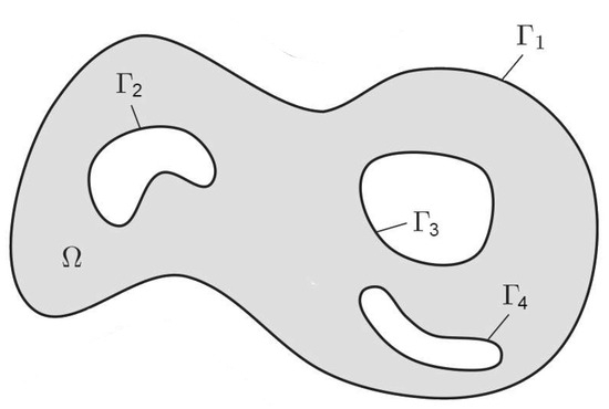
Figure 1. Domain $\mathsf{\Omega }$.

For technical reasons, we assume that ${\overline{\mathsf{\Omega }}}_1$ is contained in some bounded domain ${\mathsf{\Omega }}_0$ with the boundary $\partial {\mathsf{\Omega }}_0={\mathsf{\Gamma }}_0\in C^2$ (see Figure 2).

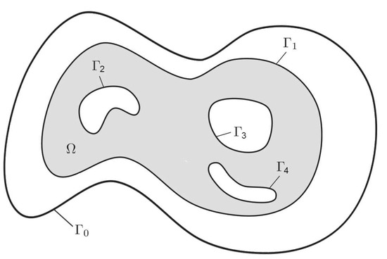
Figure 2. Domain ${\mathsf{\Omega }}_0$.

It is convenient for us to assume that the boundary $\mathsf{\Gamma }$ of the domain of $\mathsf{\Omega }$ is determined by the relation $\mathsf{\Gamma }=\{x:\mathsf{\Phi }(x)=0\}$, where the function $\mathsf{\Phi }\left(x\right)\in C^2\left({\mathsf{\Omega }}_0\right)$ and $\mathsf{\Phi }\left(x\right)>0$ for $x\in \mathsf{\Omega }$ and $\mathsf{\Phi }\left(x\right)<0$ for $x\in {\mathsf{\Omega }}_0\backslash \overline{\mathsf{\Omega }}$.

3.2. Boundary Function

We are interested in the velocity field $u\in L_2(0,T;W_2^1{\left(\mathsf{\Omega }\right)}^N))$ of an incompressible fluid that flows in the domain $\mathsf{\Omega }$ and takes the value $\alpha \left(x\right)$ on $x\in \mathsf{\Gamma }$. Here, $\alpha \left(x\right)$ is a given function. Thus, the function $u(t,x)$ satisfies the following relations

$$\mathrm{div}u(t,x)=0,(t,x)\in Q_T;$$

(12)

$$u(t,x)=\alpha \left(x\right),t\in [0,T],x\in \partial \mathsf{\Omega }.$$

(13)

From the continuity Equation (12), there follows that the function $\alpha \left(x\right)$ must satisfy the following condition

$${\int }_{\partial \mathsf{\Omega }}\alpha \left(x\right)·n\left(x\right)dx=0.$$

(14)

Here, $n\left(x\right)=(n_1\left(x\right),\cdots ,n_N\left(x\right))$ is the unit outward normal to $\partial \mathsf{\Omega }$ at point $x\in \partial \mathsf{\Omega }$,

$$\alpha \left(x\right)·n\left(x\right)=\sum _{i=1}^N{\alpha }_i\left(x\right)n_i\left(x\right).$$

The condition (14) means that the flux of the incompressible fluid across the boundary of the flow region $\mathsf{\Omega }$ is equal to zero.

Let

$$F_i={\int }_{{\mathsf{\Gamma }}_i}\alpha \left(x\right)·n\left(x\right)dx,i=1,\dots ,K,$$

(15)

be the flux of the velocity vector u across each connected component ${\mathsf{\Gamma }}_i$ of the boundary of $\mathsf{\Omega }$.

By (14), it follows that

$${\int }_{\partial \mathsf{\Omega }}\alpha \left(x\right)·n\left(x\right)dx=\sum _{i=0}^K{\int }_{{\mathsf{\Gamma }}_i}\alpha \left(x\right)·n\left(x\right)dx=\sum _{i=0}^K{F}_i=0.$$

(16)

Since the behavior of the solutions to the Cauchy problem in (11) is closely related to the boundary function $\alpha \left(x\right)$, we impose some conditions on $\alpha \left(x\right)$.

From the inclusion $u\in L_2(0,T;W_2^1{\left(\mathsf{\Omega }\right)}^N))$ it follows that for the trace $\alpha \left(x\right)$ of the function u on the boundary $\mathsf{\Gamma }$, the relation $\alpha \in W_2^{1/2}{\left(\mathsf{\Gamma }\right)}^N$ is valid.

Let us denote

$$F\left(\alpha \right)={\int }_{\mathsf{\Gamma }}\alpha \left(x\right)·n\left(x\right)dx.$$

(17)

Let us introduce the space

$$H^{1/2}\left(\mathsf{\Gamma }\right)=\{\alpha :\alpha \in W_2^{1/2}{\left(\mathsf{\Gamma }\right)}^N,F\left(\alpha \right)=0\}.$$

The function $\alpha \in H^{1/2}\left(\mathsf{\Gamma }\right)$ allows the continuation of a in $\mathsf{\Omega }$ such that $\mathrm{div}a\left(x\right)=0$ in $\mathsf{\Omega }$, $a\left(x\right)=\alpha \left(x\right)$ on $\mathsf{\Gamma }$ (see [9]), and the following inequality is true:

$${\parallel a\parallel }_{W_2^1{\left(\mathsf{\Omega }\right)}^N}\le M{\parallel \alpha \parallel }_{W_2^{1/2}{\left(\mathsf{\Gamma }\right)}^N}.$$

Denote by ${\mathsf{\Pi }}_0$ the operator that assigns to an arbitrary function $\alpha \in H^{1/2}\left(\mathsf{\Gamma }\right)$ the so constructed function $a\left(x\right)\in W{ }_2^1{\left(\mathsf{\Omega }\right)}^N$, so that ${\mathsf{\Pi }}_0\left(\alpha \right)=a$.

The function $a\in H^{1/2}\left(\mathsf{\Gamma }\right)$ allows the continuation of $a^0$ into ${\mathsf{\Omega }}_0\backslash \mathsf{\Omega }$ such that $a^0\left(x\right)=0$ on $\partial {\mathsf{\Gamma }}_0$ and $a^0\left(x\right)=\alpha \left(x\right)$ on $\mathsf{\Gamma }$ (see [9]), and the following inequality is valid:

$$\parallel a^0{\parallel }_{W_2^1{(\mathsf{\Omega }\backslash \mathsf{\Omega })}^N}{\alpha }_{W_2^{1/2}{\left(\mathsf{\Gamma }\right)}^N}.$$

Denote by ${\mathsf{\Pi }}_1$ the operator that assigns to an arbitrary function $\alpha \in H^{1/2}\left(\mathsf{\Gamma }\right)$ the so constructed function $a^0\left(x\right)\in \stackrel{\circ }{W}{ }_2^1{\left(\mathsf{\Omega }\right)}^N$, so that ${\mathsf{\Pi }}_0\left(\alpha \right)=a$.

For an arbitrary function $\alpha \in H^{1/2}\left(\mathsf{\Gamma }\right)$, the function $a^{\ast }\left(x\right)$ is defined as $a^{\ast }\left(x\right)=a\left(x\right)={\mathsf{\Pi }}_0\left(\alpha \right)$ for $x\in \mathsf{\Omega }$ and $a^{\ast }\left(x\right)=a^0\left(x\right)={\mathsf{\Pi }}_1\left(\alpha \right)$ at $x\in {\mathsf{\Omega }}_0\backslash \mathsf{\Omega }$. Obviously, $a^{\ast }\left(x\right)\in \stackrel{\circ }{W}{ }_2^1{\left({\mathsf{\Omega }}_0\right)}^N$ and

$$\parallel a^{\ast }{\parallel }_{W_2^1{\left({\mathsf{\Omega }}_0\right)}^N}\le M{\parallel \alpha \parallel }_{W_2^{1/2}{\left(\mathsf{\Gamma }\right)}^N}.$$

(18)

Denote by $\mathsf{\Pi }$ the operator that assigns to the function $\alpha \in H^{1/2}\left(\mathsf{\Gamma }\right)$ the so constructed function $a^{\ast }\left(x\right)\in \stackrel{\circ }{W}{ }_2^1{\left({\mathsf{\Omega }}_0\right)}^N$, so that $\mathsf{\Pi }\left(\alpha \right)=a^{\ast }$.

Let

$${\mathsf{\Gamma }}_{+}\left(\alpha \right)=\{x:\alpha \left(x\right)·n\left(x\right)>0,x\in \partial \mathsf{\Omega }\},$$

$${\mathsf{\Gamma }}_{-}\left(\alpha \right)=\{x:\alpha \left(x\right)·n\left(x\right)<0,x\in \partial \mathsf{\Omega }\},$$

$${\mathsf{\Gamma }}_{\ast }\left(\alpha \right)=\{x:\alpha \left(x\right)·n\left(x\right)=0,x\in \partial \mathsf{\Omega }\}.$$

Obviously, $\mathsf{\Gamma }={\mathsf{\Gamma }}_{+}\left(\alpha \right)\cup {\mathsf{\Gamma }}_{-}\left(\alpha \right)\cup {\mathsf{\Gamma }}_{\ast }\left(\alpha \right)$. Note that the sets ${\mathsf{\Gamma }}_{+}\left(\alpha \right)$, ${\mathsf{\Gamma }}_{-}\left(\alpha \right)$, and ${\mathsf{\Gamma }}_{\ast }\left(\alpha \right)$ can have a nonempty intersection with any part ${\mathsf{\Gamma }}_i$ of the boundary $\mathsf{\Gamma }$.

If ${\mathsf{\Gamma }}_{\ast }\left(\alpha \right)=\varnothing$, then $\mathsf{\Gamma }={\mathsf{\Gamma }}_{+}\left(\alpha \right)\cup {\mathsf{\Gamma }}_{-}\left(\alpha \right)$. This means that each component ${\mathsf{\Gamma }}_i$ of the boundary $\mathsf{\Gamma }$ belongs to either ${\mathsf{\Gamma }}_{+}\left(\alpha \right)$ or ${\mathsf{\Gamma }}_{-}\left(\alpha \right)$. In the case of ${\mathsf{\Gamma }}_i\subset {\mathsf{\Gamma }}_{+}\left(\alpha \right)$, the inequality $\alpha \left(x\right)·n\left(x\right)>0$ takes place on ${\mathsf{\Gamma }}_i$, and ${\mathsf{\Gamma }}_i$ is the outflow area of the fluid from $\mathsf{\Omega }$. In the case of ${\mathsf{\Gamma }}_i\subset {\mathsf{\Gamma }}_{-}\left(\alpha \right)$ the condition $\alpha \left(x\right)·n\left(x\right)<0$ takes place, which means ${\mathsf{\Gamma }}_i$ is the inflow area.

3.3. Cauchy Problem

In the case when the velocity field u of the problem (8)–(11) belongs to the space $L_2(0,T;W_2^1{\left(\mathsf{\Omega }\right)}^N)$, there is no classical solution to the Cauchy problem (11), generally speaking. Therefore, it is convenient to understand the solvability of the problem (8)–(11) in the sense of the $RLF$ theory.

However, the direct application of this theory is hindered by the presence of an inhomogeneous boundary condition ${\alpha =u|}_{\mathsf{\Gamma }}$ for function u.

To make use of the $RLF$ theory, we extend function u from $\mathsf{\Omega }$ to the wider domain ${\mathsf{\Omega }}_0$ by some function $u^{\ast }$ vanishing on ${\mathsf{\Gamma }}_0$.

Let us build this function. Let $\alpha \in H^{1/2}\left(\mathsf{\Gamma }\right)$ be a given function and let u belong to $\in L_2(0,T;W_2^1{\left(\mathsf{\Omega }\right)}^N)$ and satisfy the boundary condition ${u|}_{\mathsf{\Gamma }}=\alpha$.

Therefore, $u(t,x)$ can be represented as an element of the set of functions

$$W\left(\alpha \right)=\{u:u=v+a,u{|}_{\mathsf{\Gamma }}=\alpha \in H^{1/2}\left(\mathsf{\Gamma }\right),v\in L_2(0,T;V)\}.$$

Here, function a is the extension of $\alpha$ from $\mathsf{\Gamma }$ to $\mathsf{\Omega }$ by the ratio $a={\mathsf{\Pi }}_0\left(\alpha \right)$. The set $W\left(\alpha \right)$ is a hyperplane in $L_2(0,T;W_2^1{\left(\mathsf{\Omega }\right)}^N)$.

Let function v of variables $(t,x)\in [0,T]\times \mathsf{\Omega }$ belong to the space $L_2(0,T;V$. Extend function v from $\mathsf{\Omega }$ to ${\mathsf{\Omega }}_0\backslash \mathsf{\Omega }$ to function $v^{\ast }$ by setting $v^{\ast }(t,x)=v(t,x)$ for $x\in \mathsf{\Omega }$ and $v^{\ast }(t,x)=0$ for $x\in {\mathsf{\Omega }}_0\backslash \mathsf{\Omega }$. Denote the extension operator by ${\mathsf{\Pi }}_{+}$, so that $v^{\ast }={\mathsf{\Pi }}_{+}\left(v\right)$.

Obviously, if $u\in W\left(\alpha \right))$, then $v^{\ast }\in L_2(0,T;\stackrel{\circ }{W}{ }_2^1{\left({\mathsf{\Omega }}_0\right)}^N$.

Now, let us define the function $u^{\ast }$ on ${\mathsf{\Omega }}_0$ as $u^{\ast }=v^{\ast }+a^{\ast }$. Then, the function $u^{\ast }$ satisfies the following ratios

$$u^{\ast }(t,x)=u(t,x),x\in \mathsf{\Omega };u^{\ast }(t,x)=a^0\left(x\right),x\in {\mathsf{\Omega }}_0\backslash \mathsf{\Omega };u^{\ast }\in L_2(0,T;\stackrel{\circ }{W}{ }_2^1{\left({\mathsf{\Omega }}_0\right)}^N).$$

Along with problem (11), consider the auxiliary Cauchy problem

$$z(\tau ;t,x)=x+{\int }_t^{\tau }{u}^{\ast }(s,z(s;t,x))ds,\tau ,t\in [0,T],x\in {\mathsf{\Omega }}_0.$$

(19)

Since $u^{\ast }=v^{\ast }+a^{\ast }\in L_2(0,T;\stackrel{\circ }{W}{ }_2^1{\left({\mathsf{\Omega }}_0\right)}^N)$, we are in position to make use of the $RLF$ theory. Replacing $\mathsf{\Omega }$ by ${\mathsf{\Omega }}_0$ and making use of Theorem 5, we infer that there exists a unique $RLF$ z generated by the function $u^{\ast }=v^{\ast }+a^{\ast }$. In particular, this means that the Cauchy problem (19) has an absolutely continuous solution $z(\tau ;t,x)$ with respect to $\tau \in [0,T]$ for a.a. $x\in {\mathsf{\Omega }}_0$ and $t\in [0,T]$.

The restriction of $z(\tau ;t,x)$ from $[0,T]\times {\mathsf{\Omega }}_0$ to $[0,T]\times \mathsf{\Omega }$ yields the solutions of the Cauchy problem (11).

The function ${\tau }_u(t,x)$ is defined as

$${\tau }_u(t,x)=inf\{\tau :z(s;t,x)\in \mathsf{\Omega },s\in (\tau ,t]\},$$

where $z(s;t,x)$ is the $RLF$ generated by $u^{\ast }$.

Denote by $\mathcal{T}$ the operator that matches the function u with the function ${\tau }_u$, so that ${\tau }_u=\mathcal{T}\left(u\right)$.

4. Approximations of Functions from ${\mathit{H}}_{\mathbf{2}}^{\mathbf{1}\mathbf{/}\mathbf{2}}\mathbf{\left(}\mathsf{\Gamma }\mathbf{\right)}$

The behavior of the trajectories z of a field u in the vicinity of a boundary $\mathsf{\Gamma }$ depends significantly on the boundary function $\alpha$. Suitable approximations ${\alpha }^n$ of $\alpha$ provide the convergence of appropriate $u^n$, $z^n$, and ${\tau }^n$ to the solution u, z, and ${\tau }_u$ of original problem (8)–(11).

A complexity in the behavior of the trajectories $z^n$, and as a consequence of ${\tau }^n$, arises in a vicinity of the touch points of ${\alpha }^n$ to $\partial \mathsf{\Omega }$. Therefore, the set of such points should be small enough.

Below, we build approximations ${\alpha }^n$, whose touch-point set consists of a finite number of smooth curves on $\mathsf{\Gamma }$ in the case of $N=3$ or a finite number of points on $\mathsf{\Gamma }$ in the case of $N=2$. The use of trigonometric polynomials proves to be a convenient tool for this.

Denote by $\mathcal{A}$ the set of smooth functions $\alpha \in H^{1/2}\left(\mathsf{\Gamma }\right)$ such that the set $Z\left(\alpha \right)=\{x:\alpha (x)·n(x)=0,x\in \mathsf{\Gamma }\}$ is either empty or consists of a finite number of smooth curves on $\mathsf{\Gamma }$ in the case of $N=3$ and a finite number of points on $\mathsf{\Gamma }$ in the case of $N=2$.

Theorem 1. 

Let $\alpha \in H^{1/2}\left(\mathsf{\Gamma }\right)$. Then, for any $\epsilon >0$ there is a function ${\alpha }^{\ast }\in \mathcal{A}$ such that the following inequality is true

$$\parallel \alpha -{\alpha }^{\ast }{\parallel }_{W_2^{1/2}{\left(\mathsf{\Gamma }\right)}^N}\le \epsilon .$$

(20)

Proof of Theorem 1 (case $\mathit{N}$  = 2). 

In this case, the boundary $\mathsf{\Gamma }$ of domain $\mathsf{\Omega }$ is $\mathsf{\Gamma }={\cup }_{i=1}^K{\mathsf{\Gamma }}_i$, where ${\mathsf{\Gamma }}_i$ are smooth closed curves.

Let us take a fixed ${\mathsf{\Gamma }}_k$. Obviously, the restriction of the function $\alpha \in H^{1/2}\left(\mathsf{\Gamma }\right)$ from $\mathsf{\Gamma }$ to ${\mathsf{\Gamma }}_k$ (let us keep the designation $\alpha$ for the restriction) is such that $\alpha \in W_2^{1/2}{\left({\mathsf{\Gamma }}_k\right)}^N$.

Let the smooth function $x=q\left(s\right)$, $q\left(s\right)=(q_1\left(s\right),q_2\left(s\right))$, $s\in [0,S]$, define a parametrization of ${\mathsf{\Gamma }}_k$. Here, s means the distance along ${\mathsf{\Gamma }}_k$ from $x\left(0\right)$ to $x\left(s\right)$, and S is the length of the curve ${\mathsf{\Gamma }}_k$.

Represent the function $\alpha$ in the form $\alpha \left(x\right)={\alpha }_1\left(x\right)n\left(x\right)+{\alpha }_{2}t\left(x\right)$, where $n\left(x\right)$ is the outward unite normal, and $t\left(x\right)$, $t\left(x\right)=q^{\prime }\left(q^{-1}\left(x\right)\right)$, is the tangent vector at the point $x\in {\mathsf{\Gamma }}_k$. Then, the scalar functions ${\alpha }_i,i=1,2$ belong to the space $W_2^{1/2}\left({\mathsf{\Gamma }}_k\right)$.

Approximate the function $\alpha$ by a function ${\alpha }^{\ast }\in \mathcal{A}$.

A change of variable $q\left(s\right)=(q_1\left(s\right),q_2\left(s\right))$ converts function $\alpha \left(x\right)$ to function

$$\overline{\alpha }\left(s\right)=({\overline{\alpha }}_1\left(s\right),{\overline{\alpha }}_2\left(s\right)),{\overline{\alpha }}_i\left(s\right)={\alpha }_i(q_1\left(s\right),q_2\left(s\right)),i=1,2.$$

The inclusion $\alpha \in W_2^{1/2}{\left({\mathsf{\Gamma }}_k\right)}^N$ and the smoothness of $q\left(s\right)$ imply the inclusion $\overline{\alpha }\in W_2^{1/2}{[0,S]}^N$.

Denote by ${\mathcal{A}}^{\prime }$ the set of smooth functions $y\in W_2^{1/2}{[0,S]}^N$ such that the set

$$\overline{Z}\left(\beta \right)=\{s:y\left(s\right)=0,s\in [0,S]\}$$

is either empty or consists of a finite number of points on $[0,S$].

Lemma 1. 

Let $\overline{\alpha }\in W_2^{1/2}{[0,S]}^N$. Then, for any $\epsilon >0$, there is such a function $\widehat{\alpha }\in {\mathcal{A}}^{\prime }$ that the following inequality is true:

$$\parallel \overline{\alpha }-\widehat{\alpha }{\parallel }_{W_2^{1/2}{[0,S]}^N}\le \epsilon .$$

(21)

Proof of Lemma 1. 

We can (see [13], Section 2.1) approximate the functions ${\overline{\alpha }}_i\left(s\right)={\alpha }_i\left(q\left(s\right)\right)$, $i=1,2$, by trigonometric polynomials ${\widehat{\alpha }}_i\left(s\right)$, so that

$$\parallel \overline{\alpha }-\widehat{\alpha }{\parallel }_{W_2^{1/2}{[0,S]}^N}\le \epsilon ,\widehat{\alpha }\left(s\right)=({\widehat{\alpha }}_1\left(s\right),{\widehat{\alpha }}_2\left(s\right)).$$

(22)

Note that the set of zeros of the functions ${\widehat{\alpha }}_i$ is finite. Therefore, $\widehat{\alpha }\in {\mathcal{A}}^{\prime }$.

Lemma 1 is proved. □

Let $s=q^{-1}\left(x\right)$ be the inverse to the $x=q\left(s\right)$ map. A change of variable $s=q^{-1}\left(x\right)$ converts function $\widehat{\alpha }\left(s\right)$ to the smooth function

$${\alpha }^{+}\left(x\right)={\alpha }_1^{+}\left(x\right)n\left(x\right)+{\alpha }_2^{+}t\left(x\right),{\alpha }_i^{+}\left(x\right)={\widehat{\alpha }}_i\left(q^{-1}\left(x\right)\right).$$

From the finiteness of the set of zeros of the function ${\widehat{\alpha }}_1^{+}$ and the smoothness of $q\left(s\right)$, it follows the finiteness of the set of zeros of function ${\alpha }^{+}\left(x\right)·n\left(x\right)$ = ${\alpha }_1^{+}\left(x\right)$. Therefore, ${\alpha }^{+}\in \mathcal{A}$.

Denote

$${\beta }_k=F_k\left(\alpha \right)={\int }_{{\mathsf{\Gamma }}_k}\alpha \left(x\right)·n\left(x\right)dx={\int }_{{\mathsf{\Gamma }}_k}{\alpha }_1\left(x\right).$$

(23)

$${\beta }_k^{\prime }=F_k\left({\alpha }^{+}\right)={\int }_{{\mathsf{\Gamma }}_k}{\alpha }^{+}\left(x\right)·n\left(x\right)dx={\int }_0^S\widehat{\alpha }\left(s\right)·n(x\left(s\right)ds.$$

(24)

Let us introduce the function

$$\begin{array}{c}\hfill {\alpha }_k^{\ast }\left(x\right)={\alpha }^{+}\left(x\right)+(({\beta }_k-{\beta }_k^{\prime })/S)n\left(x\right),x\in {\mathsf{\Gamma }}_k.\end{array}$$

(25)

Note that the set of zeros of the function ${\alpha }_k^{\ast }\left(x\right)·n\left(x\right)={\alpha }^{+}\left(x\right)+((\beta -{\beta }^{\prime })/S)$ and the set of zeros of the function ${\alpha }^{+}\left(x\right)·n\left(x\right)={\alpha }^{+}\left(x\right)$ are finite.

It follows from (23)–(25) that

$$\begin{array}{c}\hfill {\beta }_k^{\ast }=F_k\left({\alpha }^{\ast }\right)={\int }_{{\mathsf{\Gamma }}_k}{\alpha }_k^{\ast }\left(x\right)·n\left(x\right)dx={\int }_{{\mathsf{\Gamma }}_k}{\alpha }_k^{+}\left(x\right)·n\left(x\right)dx+{\int }_{{\mathsf{\Gamma }}_k}(({\beta }_k-{\beta }_k^{\prime })/S)dx=\\ \hfill {\beta }^{\prime }+({\beta }_k-{\beta }_k^{\prime })={\beta }_k.\end{array}$$

(26)

Consequently,

$$\begin{array}{c}\hfill F_k\left({\alpha }^{\ast }\right)=F_k\left(\alpha \right).\end{array}$$

(27)

Estimate $\parallel \alpha -{\alpha }_k^{\ast }{\parallel }_{W_2^{1/2}\left({\mathsf{\Gamma }}_k\right)}$. Making use of (25), one has

$$\begin{array}{c}\hfill \parallel \alpha -{\alpha }_k^{\ast }{\parallel }_{W_2^{1/2}{\left({\mathsf{\Gamma }}_k\right)}^N}={\parallel \alpha \left(x\right)-{\alpha }^{+}\left(x\right)-((\beta -{\beta }^{\prime })/S)n\left(x\right)\parallel }_{W_2^{1/2}{\left({\mathsf{\Gamma }}_k\right)}^N}\le \\ \hfill \parallel \alpha -{\alpha }^{+}{\left(x\right)\parallel }_{W_2^{1/2}{\left({\mathsf{\Gamma }}_k\right)}^N}+|\beta -{\beta }^{\prime }{|/S\parallel n\left(x\right)\parallel }_{W_2^{1/2}{\left({\mathsf{\Gamma }}_k\right)}^N}=J_1+J_2.\end{array}$$

(28)

From (22) and (28), it follows that

$$\begin{array}{c}\hfill J_1=\parallel \alpha -{\alpha }^{+}{\left(x\right)\parallel }_{W_2^{1/2}{\left({\mathsf{\Gamma }}_k\right)}^N}<<{\parallel \overline{\alpha }-\widehat{\alpha }\parallel }_{W_2^{1/2}{([0,S]}^N}<M_1\epsilon .\end{array}$$

(29)

A change of the variable yields

$${\int }_{{\mathsf{\Gamma }}_k}\alpha \left(x\right)·n\left(x\right)dx={\int }_0^S\overline{\alpha }\left(s\right)·n\left(q\left(s\right)\right|q^{\prime }\left(s\right)|ds={\beta }_k.$$

(30)

$${\int }_{{\mathsf{\Gamma }}_k}\widehat{\alpha }\left(x\right)·n\left(x\left(s\right)\right)ds={\int }_0^S\widehat{\alpha }\left(s\right)·n\left(q\left(s\right)\right|q^{\prime }\left(s\right)|ds={\beta }_k^{\prime }$$

(31)

Further,

$$\begin{array}{c}\hfill J_2=|{\beta }_k-{\beta }_k^{\prime }{|/S\parallel n\left(x\right)\parallel }_{W_2^{1/2}{\left({\mathsf{\Gamma }}_k\right)}^N}\le M_2|{\beta }_k-{\beta }_k^{\prime }{|\parallel n\left(x\left(s\right)\right)\parallel }_{W_2^{1/2}{[0,S]}^N}\le M_3<|{\beta }_k-{\beta }_k^{\prime }|.\end{array}$$

(32)

From (22), (24), and (30), it follows that

$$\begin{array}{c}\hfill |{\beta }_k-{\beta }_k^{\prime }|=|{\int }_0^S(\overline{\alpha }\left(s\right)-\widehat{\alpha }\left(s\right))·n\left(x\left(s\right)\right)ds|\le M_4{\parallel \overline{\alpha }\left(s\right)-\widehat{\alpha }\left(s\right)\parallel }_{L_2{[0,S]}^N}\le \\ \hfill M_5{\parallel \overline{\alpha }\left(s\right)-\widehat{\alpha }\left(s\right)\parallel }_{W_2^{1/2}{[0,S]}^N}\le M_6\epsilon .\end{array}$$

(33)

From (29), (30) and (33), it follows that

$$\begin{array}{c}\hfill \parallel \alpha -{\alpha }_k^{\ast }{\parallel }_{W_2^{1/2}{\left({\mathsf{\Gamma }}_k\right)}^N}\le M_7\epsilon .\end{array}$$

(34)

Now, we define the function ${\alpha }^{\ast }$ on $\mathsf{\Gamma }$ by the ratio

$${\alpha }^{\ast }\left(x\right)={\alpha }_k^{\ast }\left(x\right)\mathrm{for}x\in {\mathsf{\Gamma }}_k,k=1,\dots ,K,$$

where ${\alpha }_k^{\ast }$ on each ${\mathsf{\Gamma }}_k$ is determined by the formula (25).

From inequality (34), for each ${\mathsf{\Gamma }}_k$, there follows the inequality

$$\begin{array}{c}\hfill \parallel \alpha -{\alpha }^{\ast }{\parallel }_{W_2^{1/2}{\left(\mathsf{\Gamma }\right)}^N}\le M_8\epsilon .\end{array}$$

(35)

Let us show that ${\alpha }^{\ast }$ belongs to the class $\mathcal{A}$.

Obviously, the finiteness of the set of zeros of the function ${\alpha }_k^{\ast }\left(x\right)$ implies the finiteness of the set of zeros of the function ${\alpha }^{\ast }\left(x\right)$.

It remains to prove the equality $F\left({\alpha }^{\ast }\right)=0$.

Making use of (26), we have

$$\begin{array}{c}\hfill F\left({\alpha }^{\ast }\right)={\int }_{\mathsf{\Gamma }}{\alpha }^{\ast }\left(x\right)·n\left(x\right)dx={\mathsf{\Sigma }}_{k=1}^K{\int }_{{\mathsf{\Gamma }}_k}{\alpha }_k^{\ast }\left(x\right)·n\left(x\right)dx={\mathsf{\Sigma }}_{k=1}^K{\beta }_k^{\ast }={\mathsf{\Sigma }}_{k=1}^K{\beta }_k=\\ \hfill {\int }_{\mathsf{\Gamma }}\alpha \left(x\right)·n\left(x\right)dx=F\left(\alpha \right)=0.\end{array}$$

(36)

Thus, the function ${\alpha }^{\ast }$ belongs to the class $\mathcal{A}$.

From this and the relations (35) and (36), there follows the statement of Theorem 1.

Theorem 1 is proved in the case of $N=2$. □

Proof of Theorem 1 (case $\mathit{N}$ = 3). 

In this case boundary $\mathsf{\Gamma }$ of the domain $\mathsf{\Omega }$ is $\mathsf{\Gamma }={\cup }_{i=1}^K{\mathsf{\Gamma }}_i$, where ${\mathsf{\Gamma }}_i$ are smooth surfaces.

We approximate the function $\alpha$ by the function ${\alpha }^{\ast }\in \mathcal{A}$. Recall that in the case $N=3$, the class $\mathcal{A}$ consists of smooth functions $\alpha \in H^{1/2}\left(\mathsf{\Gamma }\right)$ such that the set $Z\left(\alpha \right)=\{x:\alpha (x)·n(x)=0,x\in \mathsf{\Gamma }\}$ is either empty or consists of a finite number of smooth curves on $\mathsf{\Gamma }$ and a finite number of points.

Let us take a fixed surface ${\mathsf{\Gamma }}_k$. Consider the restriction of the function $\alpha$ defined on $\mathsf{\Gamma }$ to ${\mathsf{\Gamma }}_k$, while retaining the previous notation. Obviously, the inclusion $\alpha \in W_2^{1/2}{\left(\mathsf{\Gamma }\right)}^3$ implies the inclusion $\alpha \in W_2^{1/2}{\left({\mathsf{\Gamma }}_k\right)}^3$.

Denote by $\mathcal{B}\left({\mathsf{\Gamma }}_k\right)$ the set of smooth functions $\beta$ on ${\mathsf{\Gamma }}_k$ such that the set $Z_k\left(\beta \right)=\{x:\beta \left(x\right)·n\left(x\right)=0,x\in {\mathsf{\Gamma }}_k\}$ consists of either a finite number of smooth curves on ${\mathsf{\Gamma }}_k$ or is empty.

Lemma 2. 

Let $\beta \in W_2^{1/2}\left({\mathsf{\Gamma }}_k\right)$. Then, for any $\epsilon >0$, there is a smooth function ${\beta }_{\epsilon }\in \mathcal{B}\left({\mathsf{\Gamma }}_k\right)$ that satisfies the inequality

$$\parallel \beta -{\beta }_{\epsilon }{\parallel }_{W_2^{1/2}\left({\mathsf{\Gamma }}_k\right)}\le \epsilon .$$

(37)

Proof of Lemma 2. 

Consider the $R^3$ unit sphere

$$S=\{y:|y|=1,y=(y_1,y_2,y_3)\in R^3\}.$$

Let $p:S\to {\mathsf{\Gamma }}_k$ be a one-to-one smooth map, so that $x=p\left(y\right)$.

Let

$$y_1=cos{\phi }_{1}cos{\phi }_2,y_2=sin{\phi }_{1}cos{\phi }_2,y_3=sin{\phi }_2,{\phi }_1\in [0,2\pi ],{\phi }_2\in [0,2\pi ],$$

and define a one-to-one smooth map $q:\Xi \to S$ as $y=q\left(\phi \right)$, $\phi =({\phi }_1,{\phi }_2)$, $\Xi =[0,2\pi )\times [0,2\pi )$.

Define the map $r:\Xi \to {\mathsf{\Gamma }}_k$ by the expression $x=r\left(\phi \right)$, $r\left(\phi \right)=p\left(q\right(\phi \left)\right)$, so that it is a smooth map.

Given function $\beta \in W_2^{1/2}\left({\mathsf{\Gamma }}_k\right)$, define $\widehat{\beta }\left(\phi \right)=\beta \left(p\left(q\left(\phi \right)\right)\right)$, $\phi \in \Xi$. It is clear that $\beta \left(x\right)=\widehat{\beta }\left(r^{-1}\left(x\right)\right)$, $x\in {\mathsf{\Gamma }}_k$.

From the smoothness of the mappings $r,q$ and their inverses, it follows that $\widehat{\beta }\in W_2^{1/2}(\Xi )$.

Note that the function $\widehat{\beta }\left(\phi \right)$ defined on $\Xi$ allows a periodic continuation to $R^2$ due to the obvious relations $\widehat{\beta }(0,{\phi }_2)=\widehat{\beta }(2\pi ,{\phi }_2)$ and $\widehat{\beta }({\phi }_1,0)=\widehat{\beta }({\phi }_1,2\pi )$.

Approximate $\widehat{\beta }\left(\phi \right)$ by a non-zero trigonometric polynomial ${\widehat{\beta }}_{\epsilon }\left(\phi \right)$ (see [13], Section 2), so that

$$\parallel \widehat{\beta }-{\widehat{\beta }}_{\epsilon }{\parallel }_{W_2^{1/2}(\Xi )}\le \epsilon .$$

(38)

Due to the smoothness of the map r, the set of zeros $Z\left({\widehat{\beta }}_{\epsilon }\right)\in \Xi$ of the function ${\widehat{\beta }}_{\epsilon }\left(\phi \right)$ is either empty or may consist of a finite number of smooth curves, possibly intersecting, and a finite number of points.

Let $\widehat{z}\in W_2^{1/2}(\Xi )$ be an arbitrary function, $z\left(x\right)=z\left(r^{-1}\left(x\right)\right)$, $x\in {\mathsf{\Gamma }}_k$. The smoothness of the maps r and $r^{-1}$ implies the inequalities

$$m_1\parallel \widehat{z}{\parallel }_{W_2^{1/2}\left({\mathsf{\Gamma }}_k\right)}\le {\parallel z\parallel }_{W_2^{1/2}(\Xi )}\le m_2{\parallel \widehat{z}\parallel }_{W_2^{1/2}\left({\mathsf{\Gamma }}_k\right)}$$

(39)

for some $m_1,m_2>0$.

The inequalities (38) and (39) imply the inequality (37).

Lemma 2 is proved. □

Let $\alpha \in H^{1/2}\left(\mathsf{\Gamma }\right)$. Represent the function $\alpha \left(x\right)$ in the form

$$\alpha \left(x\right)={\alpha }_n\left(x\right)+{\alpha }_t\left(x\right).$$

Here, the normal and tangent components of $\alpha \left(x\right)$ are defined as ${\alpha }_n\left(x\right)=(\alpha \left(x\right)·n\left(x\right))n\left(x\right)$ and ${\alpha }_t\left(x\right)=\alpha \left(x\right)-{\alpha }_n\left(x\right)$, respectively, $n\left(x\right)$ is the unit outward normal to ${\mathsf{\Gamma }}_k$ at the point $x\in {\mathsf{\Gamma }}_k$.

Consider the restriction ${\alpha }_n^k$ of the function ${\alpha }_n$ to the part ${\mathsf{\Gamma }}_k$ of $\mathsf{\Gamma }$.

Making use of Lemma 2, we approximate the function ${\alpha }_n^k$ by the function ${\alpha }_n^k\left(\epsilon \right)$ so that for a predetermined $\epsilon >0$, there holds the inequality

$$\parallel {\alpha }_n^k-{\alpha }_n^k{\left(\epsilon \right)\parallel }_{W_2^{1/2}\left({\mathsf{\Gamma }}_k\right)}\le \epsilon .$$

(40)

Let function ${\alpha }_{n,\epsilon }$ be defined on $\mathsf{\Gamma }$ as having restrictions ${\alpha }_n^k\left(\epsilon \right)$ on each ${\mathsf{\Gamma }}_k$. Then, from (40), there follows

$$\parallel {\alpha }_n-{\alpha }_{n,\epsilon }{\parallel }_{W_2^{1/2}\left(\mathsf{\Gamma }\right)}\le M_9\epsilon .$$

(41)

Approximate the vector function ${\alpha }_t$ by the smooth function ${\alpha }_{t,\epsilon }$, so that the following inequality holds

$$\parallel {\alpha }_t-{\alpha }_{t,\epsilon }{\parallel }_{W_2^{1/2}{\left({\mathsf{\Gamma }}_k\right)}^3}\le \epsilon .$$

(42)

Let ${\alpha }^{\prime }={\alpha }_{n,\epsilon }+{\alpha }_{t,\epsilon }$. From inequalities (41) and (42), there follow the inclusion ${\alpha }^{\prime }\in W_2^{1/2}{\left(\mathsf{\Gamma }\right)}^3$ and the inequality

$$\parallel \alpha -{\alpha }^{\prime }{\parallel }_{W_2^{1/2}{\left({\mathsf{\Gamma }}_k\right)}^3}\le M_{10}\epsilon .$$

(43)

Let ${\sigma }_k={\int }_{{\mathsf{\Gamma }}_k}\alpha \left(x\right)·n\left(x\right)dx$, ${\sigma }_k^{\prime }={\int }_{{\mathsf{\Gamma }}_k}{\alpha }^{\prime }\left(x\right)·n\left(x\right)dx$. If ${\sigma }_k={\sigma }_r^{\prime }$, let us say ${\alpha }_k^{\ast }={\alpha }^{\prime }$, ${\sigma }_k^{\ast }={\int }_{{\mathsf{\Gamma }}_k}{\alpha }^{\ast }\left(x\right)·n\left(x\right)dx={\sigma }_k^{\prime }$. Then, from (43), there follows

$$\parallel \alpha -{\alpha }_k^{\ast }{\parallel }_{W_2^{1/2}{\left({\mathsf{\Gamma }}_k\right)}^3}\le M_{11}\epsilon .$$

(44)

If ${\sigma }_k\ne {\sigma }_k^{\prime }$, then consider the function

$$\begin{array}{c}\hfill {\alpha }_k^{\ast }={\alpha }^{\prime }+({\sigma }_k-{\sigma }_k^{\prime }){\left|{\mathsf{\Gamma }}_k\right|}^{-1}n,\end{array}$$

(45)

where $|{\mathsf{\Gamma }}_k|$ is the area of ${\mathsf{\Gamma }}_k$. Let us show that the inequality (43) holds for this ${\alpha }_k^{\ast }$.

Using the form of ${\alpha }_k^{\ast }$, we have

$$\begin{array}{c}\hfill \parallel \alpha -{\alpha }_k^{\ast }{\parallel }_{W_2^{1/2}{\left({\mathsf{\Gamma }}_k\right)}^3}\le \parallel \alpha -{\alpha }^{\prime }{\parallel }_{W_2^{1/2}{\left({\mathsf{\Gamma }}_k\right)}^3}+|{\sigma }_k-{\sigma }_k^{\prime }||{\mathsf{\Gamma }}_k{|}^{-1}{\parallel n\left(x\right)\parallel }_{W_2^{1/2}{\left({\mathsf{\Gamma }}_k\right)}^3}\le \\ \hfill \parallel \alpha -{\alpha }^{\prime }{\parallel }_{W_2^{1/2}{\left({\mathsf{\Gamma }}_k\right)}^3}+M|{\sigma }_k-{\sigma }_k^{\prime }|.\end{array}$$

(46)

Let us estimate the value of $|{\sigma }_k-{\sigma }_k^{\prime }|$. Using elementary calculations and inequality (43), we obtain

$$\begin{array}{c}\hfill |{\sigma }_k-{\sigma }_k^{\prime }|=|{\int }_{{\mathsf{\Gamma }}_k}\alpha \left(x\right)·n\left(x\right)dx-{\int }_{{\mathsf{\Gamma }}_k}{\alpha }^{\prime }\left(x\right)·n\left(x\right)dx|=|{\int }_{{\mathsf{\Gamma }}_k}(\alpha \left(x\right)-{\alpha }^{\prime }\left(x\right))·n\left(x\right)dx|\le \\ \hfill M_{12}{\int }_{{\mathsf{\Gamma }}_k}|\alpha \left(x\right)-{\alpha }^{\prime }\left(x\right))|\le M_{13}\parallel \alpha -{\alpha }^{\prime }{\parallel }_{L_2{\left({\mathsf{\Gamma }}_k\right)}^3}\le M_{14}{\parallel \alpha -{\alpha }^{\prime }\parallel }_{W_2^{1/2}{\left({\mathsf{\Gamma }}_k\right)}^3}\le M_{15}\epsilon .\end{array}$$

(47)

It follows from (45) that

$$\begin{array}{c}\hfill {\int }_{{\mathsf{\Gamma }}_k}{\alpha }_k^{\ast }\left(x\right)·n\left(x\right)dx={\int }_{{\mathsf{\Gamma }}_k}{\alpha }^{\prime }\left(x\right)·n\left(x\right)dx+({\sigma }_k-{\sigma }_k^{\prime }){\left|{\mathsf{\Gamma }}_k\right|}^{-1}{\int }_{{\mathsf{\Gamma }}_k}n\left(x\right)·n\left(x\right)dx=\\ \hfill ={\sigma }_k+({\sigma }_k-{\sigma }_k^{\prime })={\sigma }_k.\end{array}$$

(48)

Thus, ${\sigma }_k^{\ast }={\sigma }_k$.

We have shown that in the case of ${\sigma }_k\ne {\sigma }_k^{\prime }$, the inequality (43) is valid for the function ${\alpha }_k^{\ast }$, and ${\sigma }_k^{\ast }={\sigma }_k$.

Now, define the function ${\alpha }^{\ast }$ on $\mathsf{\Gamma }$ by the expression ${\alpha }^{\ast }\left(x\right)={\alpha }_k^{\ast }\left(x\right)$ for $x\in {\mathsf{\Gamma }}_k$, $k=1,\dots ,K$. The inequalities (43) for $x\in {\mathsf{\Gamma }}_k$, $k=1,\dots ,K$, imply the validity of the inequality (20).

It follows from the properties of the functions ${\alpha }_k^{\ast }$ that ${\alpha }^{\ast }\in \mathcal{A}$ and

$$F\left(\alpha \right)={\int }_{\mathsf{\Gamma }}\alpha \left(x\right)·n\left(x\right)dx={\mathsf{\Sigma }}_{k=1}^K{\int }_{{\mathsf{\Gamma }}_k}{\alpha }_k^{\ast }\left(x\right)·n\left(x\right)dx={\mathsf{\Sigma }}_{k=1}^K{\sigma }_k^{\ast }={\mathsf{\Sigma }}_{k=1}^K{\sigma }_k=0.$$

Thus, ${\alpha }^{\ast }\in H^{1/2}\left(\mathsf{\Gamma }\right)$ and satisfies the conditions of Theorem 1.

Theorem 1 is proved. □

Remark 1. 

From Theorem 1, it follows that an arbitrary function $\alpha \in H^{1/2}\left(\mathsf{\Gamma }\right)$ can be approximated by the sequence ${\alpha }^n\in \mathcal{A}$, $n=1,2,\dots .$, such, that the ratio ${lim}_{n\to +\infty }{\parallel \alpha -{\alpha }^n\parallel }_{H^{1/2}\left(\mathsf{\Gamma }\right)}=0$ holds. Let us move on to studying the properties of the initial function.

5. Initial Function (Case $\mathit{u}\mathbf{\in }{\mathit{C}}^{\mathbf{2}}\mathbf{\left(}\overline{{\mathit{Q}}_{\mathit{T}}}\mathbf{\right)}$)

5.1. The Case of ${\mathsf{\Gamma }}_{\ast }=\varnothing$

Let $u\in C^2\left(\overline{Q_T}\right)$, the condition (13) be satisfied on $\partial \mathsf{\Omega }$, and $\alpha \in \mathcal{A}$. Let us continue the function u in a smooth way from $\mathsf{\Omega }$ in ${\mathsf{\Omega }}_0$ so that the continuation of $u^{\ast }$ to ${\mathsf{\Gamma }}_0$ vanishes. Then, $u^{\ast }\in C^2\left(\overline{Q}\right)$.

Along with problem (3), consider the Cauchy problem

$$z(\tau ;t,x)=x+{\int }_t^{\tau }{u}^{\ast }(s,z(s;t,x))ds,\tau ,t\in [0,T],x\in {\mathsf{\Omega }}_0.$$

(49)

Since $u^{\ast }$ vanishes on $\partial {\mathsf{\Omega }}_0$ and $u^{\ast }\in C^2\left(\overline{Q}\right)$, the Cauchy problem (49) is uniquely solvable, and its solution $z(\tau ;t,x)$ is defined for all $\tau \in [0,T]$ and is continuously differentiable on $\overline{Q}$.

In accordance with (4), the initial function ${\tau }_u(t,x)$ for solution $z(\tau ;t,x)$ to the Cauchy problem (49), we define the omitting index u by the ratio

$$\tau (t,x)=inf\{\tau :z(s;t,x))\in \overline{\mathsf{\Omega }},s\in (\tau ,t]\},t,\in [0,T],x\in \overline{\mathsf{\Omega }}.$$

(50)

The behavior of the function $\tau (t,x)$ depends on the behavior of the boundary function $\alpha \left(x\right)$ on $\mathsf{\Gamma }$ at the tangent points.

Theorem 2. 

Let the set ${\mathsf{\Gamma }}_{\ast }\left(\alpha \right)=\varnothing$. Then, the function $\tau (t,x)$ is continuous on $Q_T$.

Proof of Theorem 2. 

Let $(t,x)\in Q_T$. Denote ${\tau }^{\ast }=\tau (t,x)$, $z^{\ast }=z(\tau (t,x);t,x)$. Then, $z^{\ast }=z({\tau }^{\ast };t,x)$.

At first, consider the case when ${\tau }^{\ast }>0$. In this case, $z^{\ast }\in \partial \mathsf{\Omega }=\mathsf{\Gamma }$. Otherwise, $z\left(\tau \right(t,x);t,x)$ could be continued to the left of ${\tau }^{\ast }>0$. Therefore, $\mathsf{\Phi }\left(z^{\ast }\right)=0$.

Since $z(\tau ;t,x)\in \mathsf{\Omega }$ at $\tau \in ({\tau }^{\ast },t)$ and $z^{\ast }\in \mathsf{\Gamma }$, then trajectory $z(\tau ;t,x)$ enters $\mathsf{\Omega }$ at point $z^{\ast }$,

$$dz({\tau }^{\ast };t,x)/d\tau =u({\tau }^{\ast },z({\tau }^{\ast };t,x))=u({\tau }^{\ast },z^{\ast })=\alpha \left(z^{\ast }\right)$$

and $\alpha \left(z^{\ast }\right)·n\left(z^{\ast }\right)<0$. Therefore, $z^{\ast }$ belongs to the set ${\mathsf{\Gamma }}_{-}\left(\alpha \right)$.

Consider the function $\mathsf{\Psi }(\tau ,t,x)=\mathsf{\Phi }\left(z\right(\tau ;t,x\left)\right)$. The ratio $\mathsf{\Psi }(\tau ,t,x)=0$ defines $\tau$ as an implicit function of variables $(t,x)$. Indeed, it is not difficult to see that

$$\partial \mathsf{\Psi }({\tau }^{\ast },t,x)/\partial \tau =\nabla \mathsf{\Phi }\left(z^{\ast }\right)·u({\tau }^{\ast },z^{\ast })=0.$$

Since the vector $\nabla \mathsf{\Phi }\left(z^{\ast }\right)$ is proportional to the normal vector $n\left(z^{\ast }\right)$, then, by virtue of boundary condition (13) and the inclusion of $z^{\ast }\in {\mathsf{\Gamma }}_{-}\left(\alpha \right)$, it follows that

$$\partial \mathsf{\Psi }({\tau }^{\ast },t,x)/\partial \tau =\nabla \mathsf{\Phi }\left(z^{\ast }\right)·\alpha \left(z^{\ast }\right)<0.$$

Therefore (see [14], Section Ch. 9, p. 223), there exists the implicit function $\tau$ of variables $\tau (t,x)$ which is continuously differentiable in the neighborhood of $(t,x)$ and even more continuous. It is clear that this function $\tau =\tau (t,x)$.

Now, let ${\tau }^{\ast }=0$. In this case, either $z^{\ast }\in \partial \mathsf{\Omega }$ or $z^{\ast }\in \mathsf{\Omega }$. In the first case, by virtue of the condition of Theorem 2, $z^{\ast }$ belongs to the set ${\mathsf{\Gamma }}_{-}\left(\alpha \right)$, and the proof is similar to the one performed above.

Consider the case of $z^{\ast }\in \mathsf{\Omega }$. From the continuity of $z(\tau ;t,x)$ according to the initial data (see [1], Section V.2), it follows that there is such a small neighborhood U of the point $(t,x)$ that for $(t^{\prime },x^{\prime })\in U$, the solution of the Cauchy problem $z(0;t^{\prime },x^{\prime })$ differs little from $z^{\ast }\in \mathsf{\Omega }$. Then, $\tau (t^{\prime },x^{\prime })=0$ for $(t^{\prime },x^{\prime })\in U$, and therefore, $\tau (t,x)$ is continuous at point $(t,x)$.

Theorem 2 is proved. □

Let us now consider the case of a nonempty set ${\mathsf{\Gamma }}_{\ast }\left(\alpha \right)$. In this case, the function $\tau =(t,x)$, generally speaking, is not continuous on $Q_T$. Let us give an example.

5.2. An Example of a Discontinuous Function $\tau (t,x)$

The continuity of the function $u\in C^2\left(\overline{Q_T}\right)$ does not guarantee the continuity of the function $\tau (t,x)$ by $Q_T$. Let the domain be $\mathsf{\Omega }\in R^2$, $\mathsf{\Omega }=\{(x_1,x_2):x_1\in R^1,\parallel x_2|\le 1\}$.

Consider the Cauchy problem

$$\begin{array}{c}\hfill d{z}_1(\tau ;t,x)/d\tau =z_2(\tau ;t,x))\tau \in [0,T],t\in [0,T],x=(x_1,x_2)\in \overline{\mathsf{\Omega }},\\ \hfill d{z}_2(\tau ;t,x)/d\tau =-z_1(\tau ;t,x))\tau \in [0,T],t\in [0,T],x\in \overline{\mathsf{\Omega }},\\ \hfill z_1(t;t,x)=x_1,z_2(t;t,x)=x_2,\end{array}$$

(51)

or, equivalently, the integral Equation (3), where $u=(x_2,-x_1)$, $z=(z_1,z_2)$.

Obviously, the Cauchy problem (51) is uniquely solvable for any $(t,x)\in Q_T$.

Let $t=\pi$, $x=(1,0)$. Then, $z=(z_1,z_2)$, where $z_1=sin\tau$ and $z_2=cos\tau$, is the solution to the Cauchy problem (51).

Obviously, $z(\tau ;\pi ,x)\in \mathsf{\Omega }$ for $\pi /2\tau \le \pi$ and $z(\pi /2;\pi ,x)\in \partial \mathsf{\Omega })$. This means that trajectory $z(\tau ;t,x)$ which comes out from $x=(1,0)$ at moment $t=\pi$ get on the boundary of the $\mathsf{\Omega }$ at moment $t=\pi /2$. Therefore, $\tau (t,x)=\pi /2$ for $t=\pi$, $x=(1,0)$.

Now, let $x=x^{\prime }=(x_1^{\prime },0)$, $x_1^{\prime }\in (1-\delta ,1)$, where $\delta >0$ is quite small. Then, $z(\tau ;\pi ,x^{\prime })=(1-\delta )(sin\tau ,cos\tau )$ is a solution to the Cauchy problem (51) with the initial condition $t=\pi$, $x=x^{\prime }$. In this case, $\left|z\right(\tau ;\pi ,x^{\prime }\left)\right|=1-\delta <1$, and then $z(\tau ;\pi ,x^{\prime })\in \mathsf{\Omega }$ for all $\tau \in [0,\pi ]$. Therefore, $\tau (t,x)=0$ for $t=\pi$, $x^{\prime }=(1-\delta ,0)$.

Now, let us say $x_1^{\prime }\in (1+\delta ,1)$, where $\delta >0$ is quite small. Then, $z(\tau ;\pi ,x^{\prime })=(1+\delta )(sin\tau ,cos\tau )$ is a solution to the Cauchy problem (51) with the initial condition $x=x^{\prime }$. In this case, $\left|z\right(\tau ;\pi ,x^{\prime }\left)\right|=1+\delta >1$, since when decreasing $\tau \in [\pi /2,\pi ]$ function $z_1(\tau ;\pi ,x^{\prime })$ decreases while $z_2(\tau ;\pi ,x^{\prime })$ increases. Therefore, there is such a ${\tau }^{\ast }\in (\pi /2,\pi )$ that $z(\tau ;\pi ,x^{\prime })\in \mathsf{\Omega }$ when $\tau \in ({\tau }^{\ast },\pi ]$, and $z(\tau :\ast ;\pi ,x)\in \mathsf{\Gamma })$. Consequently, $\tau (t,x)>\pi /2$ for $t=\pi$, $x^{\prime }=(1+\delta ,0)$.

It is easy to show that for $x_1^{\prime }\in (1+\delta ,1)$ and $\delta \to 0$, ${lim}_{x^{\prime }\to +x}\tau (t,x^{\prime })=\pi /2$.

Thus, when $x^{\prime }$ tends to x on the left and right, the function ${\tau }_u(t,x^{\prime })$ has limits 0 and $\pi /2$, respectively. Therefore, $\tau (t,x)$ is discontinuous at the point $(t,x)$ for $t=\pi$, $x=(1,0)$.

Note that the unboundedness of the domain in this example is a technical point, and in the case of a bounded domain, it is not difficult to construct a similar example.

5.3. Case of a Nonempty ${\mathsf{\Gamma }}_{\ast }\left(\alpha \right)$

Let $z(\tau ;t,x)$ be the solution to the Cauchy problem (3). Consider the set

$$Q_{\ast }=\{(t,x):(t,x)\in Q_T,x=z(\tau ;t^{\ast },x^{\ast }),{\tau }^{\ast }\in [0,T],x^{\ast }\in {\mathsf{\Gamma }}_{\ast }\left(\alpha \right),T\ge t\ge {\tau }^{\ast }\}.$$

The set $Q_{\ast }$ is the image of $[0,T]\times {\mathsf{\Gamma }}_{\ast }$ into $Q_T$ by the mapping $(t^{\ast },x^{\ast })\to (t,z(t;t^{\ast },x^{\ast }))$.

Since $\alpha \in \mathcal{A}$, then $m\left(Q_{\ast }\right)=0$, where $m\left(Q_{\ast }\right)$ is the Lebesgue measure of the set $Q_{\ast }$ in $R^{N+1}$.

Let $Q_{+}\left(\alpha \right)=Q_T\backslash Q_{\ast }$. Obviously, $m\left(Q_{+}\left(\alpha \right)\right)=m\left(Q_T\right)$.

Theorem 3. 

Let the set ${\mathsf{\Gamma }}_{\ast }\left(\alpha \right)\ne \varnothing$. Then, the function $\tau (t,x)$ is continuous on $Q_{+}\left(\alpha \right)$.

Proof of the Theorem 3. 

Let $(t,x)\in Q_{+}\left(\alpha \right)$. Then, $(t,x)\notin Q_{\ast }$, and therefore, $z^{\ast }=z(\tau (t,x);t,x)\notin {\mathsf{\Gamma }}_{\ast }\left(\alpha \right)$. Consequently, $z^{\ast }\in {\mathsf{\Gamma }}_{-}\left(\alpha \right)$. The proof of the continuity of the function $\tau (t,x)$ in the vicinity of a given point $(t,x)$ is carried out in the same way as in the proof of Theorem 2 in the situation $z^{\ast }\in {\mathsf{\Gamma }}_{-}\left(\alpha \right)$.

Theorem 3 is proved. □

Let us move on to studying the properties of the initial function in the general case.

6. Initial Function (Case $\mathit{u}\mathbf{\in }{\mathit{L}}_{\mathbf{2}}\mathbf{(}\mathbf{0}\mathbf{,}\mathit{T}\mathbf{;}{\mathit{W}}_{\mathbf{2}}^{\mathbf{1}}{\mathbf{\left(}\mathsf{\Omega }\mathbf{\right)}}^{\mathit{N}}\mathbf{)}$)

6.1. Approximations of the Velocity Field

Let $u\in L_2(0,T;W_2^1{\left(\mathsf{\Omega }\right)}^N))$ and satisfy inhomogeneous condition (13) on boundary $\mathsf{\Gamma }$ and condition (12). Represent u in the form $u=v+a$, where $v\in L_2(0,T;V)$, and $a={\mathsf{\Pi }}_0\left(\alpha \right)$ is the continuation of $\alpha$ from $\mathsf{\Gamma }$ into $\mathsf{\Omega }$.

Consider the set of functions:

$$W=\{u:u=v+a,v\in L_2(0,T;V),a={\mathsf{\Pi }}_0\left(\alpha \right)\}.$$

Let u be an arbitrary function from W. Approximate function u by a sequence of smooth functions via approximations v and a.

Denote by $\mathcal{P}$ the “Leray projector”, i.e., the orthogonal projector in $L_2{(\mathsf{\Omega })}^N)$ onto the space H of divergence-free functions.

Consider the operator $Av=-\mathcal{P}\mathrm{Div}\mathcal{E}\left(v\right)$, which acts in H and is defined on the domain $D\left(A\right)=W_2^2{\left(\mathsf{\Omega }\right)}^N\cap \stackrel{\circ }{W}{ }_2^1{\left(\mathsf{\Omega }\right)}^N\cap H$.

The operator A is a positively definite self-adjoint operator (see [15], Section 2.4) The orthogonal system of eigenvectors $e_1,e_2,\dots$ with eigenvalues $0<{\lambda }_1,{\lambda }_2,\dots$ forms an orthonormal basis in H.

Let $u\in W$, $u=v+a$, $v\in L_2(0,T;V)$. Represent function v in the form

$$v(t,x)=\sum _{k=1}^{+\infty }{g}_k\left(t\right)e_k\left(x\right),$$

(52)

where $g_k\left(t\right)=(v(t,x),e_k\left(x\right))$.

Then,

$${\parallel v\parallel }_0^2=\sum _{k=1}^{+\infty }{\parallel g_k\left(t\right)\parallel }_{L_2[0,T]}^2,n=1,2,\dots ,$$

(53)

$${\parallel v\parallel }_{0,1}^2=\sum _{k=1}^{+\infty }{\lambda }_k{\parallel g_k\left(t\right)\parallel }_{L_2[0,T]}^2,n=1,2,\dots .$$

(54)

Consider the sequence of approximate functions $v^n$:

$$v^n(t,x)=\sum _{k=1}^n{g}_k\left(t\right)e_k\left(x\right),$$

(55)

where $g_k\left(t\right)=(v(t,x),e_k\left(x\right))$.

The following equalities are valid:

$$\parallel v^n{\parallel }_0^2=\sum _{k=1}^n{\parallel g_k\left(t\right)\parallel }_{L_2[0,T]}^2,n=1,2,\dots ,$$

(56)

$$\parallel v^n{\parallel }_{0,1}^2=\sum _{k=1}^n{\lambda }_k{\parallel g_k\left(t\right)\parallel }_{L_2[0,T]}^2,n=1,2,\dots .$$

(57)

Then,

$$\parallel v^n{\parallel }_0\le {\parallel v\parallel }_0,\parallel v^n{\parallel }_{0,1}\le {\parallel v\parallel }_{0,1},n=1,2,\dots ,$$

(58)

and the convergence is valid:

$$\parallel v-v^n{\parallel }_0\to 0,n\to +\infty ,{\parallel v-v^n\parallel }_{0,1}\to 0,n\to +\infty .$$

(59)

It follows from Theorem 1 that there exists a sequence ${\alpha }^n\in \mathcal{A}$ such that $\parallel \alpha -{\alpha }^n{\parallel }_{W_2^{1/2}{\left(\mathsf{\Gamma }\right)}^N}$→ 0 as $n\to +\infty$. Let $a^n={\mathsf{\Pi }}_0\left({\alpha }^n\right)$. Then, $\parallel a-a^n{\parallel }_{W_2^1{\left(\mathsf{\Omega }\right)}^N}\to 0$ as $n\to +\infty$.

Denote by $v^{n,\ast }$ and $v^{\ast }$ the extensions of the functions $v^n$ and v, respectively, from $\mathsf{\Omega }$ to ${\mathsf{\Omega }}_0$, and put

$$u^{n,\ast }(t,x)=v^{n,\ast }(t,x)+a^n\left(x\right),$$

(60)

$$u^{\ast }(t,x)=v^{\ast }(t,x)+a^n\left(x\right).$$

(61)

Obviously,

$$u^{\ast }=uin\mathsf{\Omega },u=ain{\mathsf{\Omega }}_0\backslash \mathsf{\Omega },u^{n,\ast }=u^{n}in\mathsf{\Omega },u^n=a^{n}in{\mathsf{\Omega }}_0\backslash \mathsf{\Omega }$$

and

$$u^{\ast },u^{n,\ast }\in L_2(0,T;\stackrel{\circ }{W}{ }_2^1{\left({\mathsf{\Omega }}_0\right)}^N).$$

It follows from (58)–(59) that

$$\parallel u^n{\parallel }_0\le M_0,{\parallel u^n\parallel }_{0,1}\le M_0,n=1,2,\dots ,$$

(62)

for some constant $M_0$, and the convergence is valid:

$$\parallel u^{\ast }-u^{n,\ast }{\parallel }_{L_2(0,T;L_2{\left({\mathsf{\Omega }}_0\right)}^N)}\to 0,n\to +\infty ,{\parallel u^{\ast }-u^{n,\ast }\parallel }_{L_2(0,T;\stackrel{\circ }{W}{ }_2^1{\left({\mathsf{\Omega }}_0\right)}^N)}\to 0,n\to +\infty .$$

(63)

Along with the Cauchy problem (19), consider the Cauchy problem (19)

$$\begin{array}{c}\hfill z^n(\tau ;t,x)=x+{\int }_t^{\tau }{u}^{n,\ast }(s,z^n(s;t,x))ds,\tau ,t\in [0,T],x\in {\mathsf{\Omega }}_0.\end{array}$$

(64)

Since $u^{\ast },u^{n,\ast }\in L_2(0,T;\stackrel{\circ }{W}{ }_2^1{\left({\mathsf{\Omega }}_0\right)}^N)$, then there are uniquely definable $RL{F}^{\prime }s$ $z(s;t,x)$ and $z^n(s;t,x)$ generated by the functions $u^{\ast }$ and $u^{n,\ast }$, respectively (see Theorem 5).

It follows from Theorem 6 that the sequence of $RLF$ $z^n(s;t,x)$ converges (up to a subsequence) with respect to $(s,x)$ in $Q=[0,T]\times {\mathsf{\Omega }}_0$-measure to $RLF$ $z(s;t,x)$ generated by $u^{\ast }$ uniformly over t.

Then, there is a subsequence $z^n(s;t,x)$, which, for a.a. $(s,x)\in Q_T$, converges to $z(s;t,x)$ by $[0,T]\times {\mathsf{\Omega }}_0$ uniformly over t.

Let us assume that this is the sequence $z^n(s;t,x)$ itself.

Consider now the initial functions defined on $Q_T$

$${\tau }^n(t,x)=inf\{\tau :z^n(s;t,x))\in \mathsf{\Omega },s\in (\tau ,t]\},$$

(65)

$$\tau (t,x)=inf\{\tau :z(s;t,x\left)\right)\in \mathsf{\Omega },s\in (\tau ,t]\},$$

(66)

for the aforementioned $z^n(s;t,x)$ and $z(s;t,x)$.

Find out some properties of the functions $\tau (t,x)$ and ${\tau }^n(t,x)$.

6.2. Limit Function $\tau (t,x)$

Let $u\in W$. It follows from Section 6.1 that there are smooth approximations of the function u by the functions $u^{n,\ast }$. Let $z^n(\tau ;t,x)$, $(t,x)\in Q_T$ be a solution to the Cauchy problem (64).

First of all, we note that from (60), it follows that the function $u^{n,\ast }$ is continuous and differentiable on $Q=[0,T]\times {\mathsf{\Omega }}_0$. Then, $RLF$ $z^n(\tau ;t,x)$ is a classical solution to the ODE system (64).

The continuous dependence of the solutions of the ODE system with respect to the initial data $(t,x)$ (see [1], Section V.3) implies the continuity of the function $z^n(\tau ;t,x)$ on $G_0$.

It follows from Theorem 2 that for the function ${\tau }^n(t,x)$ defined by relation (65), the following sentence is valid:

Lemma 3. 

Let ${\mathsf{\Gamma }}_{\ast }\left({\alpha }^n\right)=\varnothing$. Then, the function ${\tau }^n(t,x)$ is continuous on $Q_T$.

Moreover, making use of Theorem 3, one obtains

Lemma 4. 

Let ${\mathsf{\Gamma }}_{\ast }\left({\alpha }^n\right)\ne \varnothing$. Then, the function ${\tau }^n(t,x)$ is continuous on $Q_{+}\left({\alpha }^n\right)$.

We make use of these statements to prove the following fact.

Theorem 4. 

The sequence ${\tau }^n(t,x)$ converges (up to the subsequence) to $\tau (t,x)$ as $n\to +\infty$ at a.a. $(t,x)\in Q_T$.

Proof of Theorem 4. 

Since $m\left(Q_{+}\left({\alpha }^n\right)\right)=m\left(Q_T\right)$, $m\left({\cap }_{n=1}^{+\infty }{Q}_{+}\left({\alpha }^n\right)\right)=m\left(Q_T\right)$. Consequently, ${\tau }^n(t,x)$, $n=1,2,\dots$ are continuous on the set ${\cap }_{n=1}^{+\infty }{Q}_{+}\left({\alpha }^n\right)$, which is dense in $Q_T$.

From the convergence of the sequence $z^n(s;t,x)$ to $z(s;t,x)$ at a.a. $(s,x)\in Q_T$, it follows that at a.a. $x\in \mathsf{\Omega }$, convergence takes place at a.a. $s\in [0,T]$. Let us choose such an x. Then, the sequence $z^n(s;t,x)$ converges to $z(s;t,x)$ at a.a. $s\in [0,T]$.

Let us show that then, ${\tau }^n(t,x)$ converges to $\tau (t,x)$.

Suppose that $\tau (t,x)>0$ and assume the opposite, i.e., ${\tau }^n(t,x)$ does not converge to ${\tau }^{\ast }(t,x)$. Then, there is a subsequence $z^n(s;t,x)$ (the indices are the same), in which either ${\tau }^n(t,x)>\tau (t,x)+\delta$ or ${\tau }^n(t,x)<\tau (t,x)-\delta$ for some $\delta >0$.

First, let ${\tau }^n(t,x)>\tau (t,x)+\delta$. Let us choose ${\tau }_1>\tau (t,x)+\delta$ so that $z^n({\tau }_1;t,x)$ converges to $z({\tau }_1;t,x)$. Then, $z({\tau }_1(t,x);t,x)\in \mathsf{\Omega }$ when ${\tau }_1=\tau (t,x)+\delta$ and $\mathsf{\Phi }\left(z({\tau }_1(t,x);t,x)\right)<0$, while $z^n({\tau }_1(t,x);t,x)\notin \mathsf{\Omega }$ and $\mathsf{\Phi }\left(z^n({\tau }_1(t,x);t,x)\right)>0$.

A passage to the limit in the last inequality yields $\mathsf{\Phi }\left(z({\tau }_1(t,x);t,x)\right)\ge 0$, which cannot be.

Similarly, the case of ${\tau }^n(t,x)<\tau (t,x)-\delta$ is considered.

In the case $\tau (t,x)>0$, Theorem 4 is proved.

The case $\tau (t,x)=0$ is proved more simply.

Theorem 4 is proved. □

Corollary 1. 

The function $\tau (t,x)\in L_{\infty }\left(Q\right)$. The measurability of $\tau (t,x)$ follows from Theorem 4 and the boundedness is obvious.

7. Regular Lagrangian Flows

Here are the facts used above from the theory of $RLF$ (see, for example, [16,17,18]).

Definition 1. 

Let $u\in L_1(0,T;\stackrel{\circ }{W}{ }_p^1{\left(\mathsf{\Omega }\right)}^N)$, ${u|}_{[0,T]\times \partial \mathsf{\Omega }}=0$. Associated to u, a regular Lagrangian flow is the function $z(\tau ;t,x)$, $(\tau ;t,x)\in [0,T]\times [0,T]\times \overline{\mathsf{\Omega }}$, which satisfies the following conditions:

(1) For a.a. x and any $t\in [0,T]$, the function $z(\tau ;t,x)$ is absolutely continuous with respect to τ and satisfies the equation

$$z(\tau ;t,x)=x+{\int }_t^{\tau }u(s,z(s;t,x))ds,\tau \in [0,T];$$

(67)

(2) For any $t,\tau \in [0,T]$ and an arbitrary Lebesgue measurable set B, the relation is valid $m\left(z\right(\tau ;t,B\left)\right)\le Mm\left(B\right),M>0;$

(3) For all $t_i,\in [0,T],i=1,2,3$, and a.a. $x\in \overline{\mathsf{\Omega }}$

$$z(t_3;t_1,x)=z(t_3;t_2,z(t_2;t_1,x)).$$

Here, $m\left(B\right)$ is a Lebesgue measure of the set B.

Let us recall some results on $RLF$.

Theorem 5. 

Let $u\in L_1(0,T;\stackrel{\circ }{W}{ }_p^1{\left({\mathsf{\Omega }}_0\right)}^N)$, $1\le p\le +\infty$. Then, there exists a unique z generated by v. Moreover,

$$\frac{\partial }{\partial \tau }z(\tau ;t,x)=u(\tau ,z(\tau ;t,x))\mathrm{at}t\in [0,T],\mathrm{a}.\mathrm{a}.\tau \in [0,T],\mathrm{a}.\mathrm{a}.x\in {\mathsf{\Omega }}_0,$$

$$m\left(z\right(\tau ;t,B)\le Mm(B),M>0,\mathit{for}\mathit{any}\mathit{Lebesgue}\mathit{measurable}\mathit{set}B\subset \mathsf{\Omega }.$$

Theorem 6. 

Let v, $v^m\in L_1(0,T;\stackrel{\circ }{W}{ }_p^1{\left({\mathsf{\Omega }}_0\right)}^N)$, $m=1,2,\dots$ for some $p>1$. Let the inequalities be fulfilled

$$\parallel v_x{\parallel }_{L_1(0,T;L_p{\left({\mathsf{\Omega }}_0\right)}^{2\times 2})}+{\parallel v\parallel }_{L_1(0,T;L_1{\left({\mathsf{\Omega }}_0\right)}^N)}\le M,\parallel v_x^m{\parallel }_{L_1(0,T;L_p{\left({\mathsf{\Omega }}_0\right)}^{N\times N})}+{\parallel v^m\parallel }_{L_1(0,T;L_1{\left({\mathsf{\Omega }}_0\right)}^2)}\le M.$$

Let $v^m$ converge to v in $L_1{\left(Q\right)}^m$ for $m\to +\infty$. Let $z^m(\tau ;t,x)$ and $z(\tau ;t,x)$ be the $RLF$s generated by $v^m$ and v, respectively. Then, the sequence $z^m$ converges (up to the subsequence) to z with respect to a Lebesgue measure on the set $[0,T]\times {\mathsf{\Omega }}_0$ uniformly on $t\in [0,T]$.

For $x\in \overline{\mathsf{\Omega }}$ and $0\le \tau \le t$, the trajectory $z(\tau ;t,x)$ belongs to the domain $\overline{\mathsf{\Omega }}$, unless $\tau \in [{\tau }_u(t,x),t]$, ${\tau }_u(t,x)=inf\{\tau :z(s;t,x))\in \mathsf{\Omega },s\in (\tau ,t]\}$.

From the definition of the function ${\tau }_u(t,x)$, it follows that $z(\tau ;t,x)\in \mathsf{\Omega }$ at $\tau \in \left(\tau \right(t,x),t]$, and $z\left(\tau \right(t,x);t,x)\in \partial \mathsf{\Omega }$ when $\tau (t,x)>0$.

It is clear that for all $t\in [0,T]$, a.a. $x\in \mathsf{\Omega }$ and ${\tau }_u(t,x)\le \tau \le t$, the function $z(\tau ;t,x)$ satisfies Equation (67).

Note that in the case of a smooth $u(t,x)$, the $RLF$ $z(\tau ;t,x)$ is a classical solution of the Cauchy problem (67).

8. Conclusions

The approximations of a divergence-free velocity field $u\in L_1(0,T;W_2^1{\left(\mathsf{\Omega }\right)}^N)$ with an inhomogeneous condition on the boundary of a bounded multi-connected domain $\mathsf{\Omega }$ by a sequence of smooth fields $u^n$ were constructed. By this, the smooth trajectories $z^n(\tau ;t,x)$ of the fields $u^n$ were defined on the maximal intervals $({\tau }_u^n(t,x),{\overline{\tau }}_u^n(t,x))$, where initial functions ${\tau }_u^n(t,x)$ were continuously differentiable a.e. and $z^n(\tau ;t,x)$ and ${\tau }_u^n(t,x)$ converged a.e. to the trajectories $z(\tau ;t,x)$ generated by the regular Lagrangian flow u and initial function ${\tau }_u(t,x)$ of the field u, respectively.

A commonly used method for solving systems of type (8)–(11) consists in approximating them with a sequence of regularized systems, the solutions $u^n$ of which, together with the $z^n$ and ${\tau }^n$ generated by them, satisfy the integral identity defining the weak solution. The proposed method of regularization of the original field u provides the necessary properties of functions $u^n$, $z^n$, and ${\tau }^n$ for the limit passage to u, z, and ${\tau }_u$, respectively. This takes into account the inhomogeneity of the condition on u at the boundary of the multi-connected domain and the belonging of u to the Sobolev space.

References

- Hartman, P. Ordinary Differential Equations, 2nd ed.; Birkhauser: Boston, MA, USA, 1982. [Google Scholar]
- Zvyagin, V.G.; Vorotnikov, D.A. Topological Approximation Methods for Evolutionary Problems of Nonlinear Hydrodynamics; Walter de Gruyter & Co.: Berlin, Germany, 2008. [Google Scholar]
- Zvyagin, V.G.; Orlov, V.P. On the solvability of the initial boundary value problem for one model of viscoelasticity with fractional derivatives. Sib. Math. J. 2018, 59, 1073–1089. [Google Scholar] [CrossRef]
- Zvyagin, V.G.; Dmitrienko, V.T. On weak solutions of the initial boundary value problem for a regularized model of a viscoelastic fluid. Differ. Equ. 2002, 38, 1731–1744. [Google Scholar] [CrossRef]
- Zvyagin, V.G.; Orlov, V.P. On the weak solvability of the viscoelasticity problem with memory. Differ. Equ. 2017, 53, 212–217. [Google Scholar] [CrossRef]
- Zvyagin, V.G.; Orlov, V.P. The weak solvability of an inhomogeneous dynamic problem for a viscoelastic continuum with memory. Funct. Anal. Its Appl. 2023, 57, 74–79. [Google Scholar] [CrossRef]
- Zvyagin, V.G.; Orlov, V.P. On weak solvability of a flow problem for viscoelastic fluid with memory. Comput. Math. Math. Phys. 2023, 63, 2090–2106. [Google Scholar] [CrossRef]
- Orlov, V.P. A non-homogeneous regularized problem of dynamics of viscoelastic continuous medium. Russ. Math. 2012, 56, 48–53. [Google Scholar] [CrossRef]
- Korobkov, M.V.; Pileckas, K.; Pukhnachov, V.V.; Russo, R. The flux problem for the Navier-Stokes equations. Russ. Math. Surv. 2014, 69, 1065–1122. [Google Scholar] [CrossRef]
- Zvyagin, V.G.; Orlov, V.P. The problem of the flow of one type of non-Newtonian fluid through the boundary of a multi-connected domain. Dokl. Math. 2023, 107, 112–116. [Google Scholar] [CrossRef]
- Krein, S.G. Functional Analysis; Wolters-Noordhoff Publishing: Groningen, The Netherlands, 1972. [Google Scholar]
- Temam, R. Navier-Stokes Equations. Theory and Numerical Analysis; North-Holland Publishing Company: Amsterdam, The Netherlands; New York, NY, USA; Oxford, UK, 1979. [Google Scholar]
- Nikol’skii, S.M. Approximation of Functions of Several Variables and Imbedding Theorems; Springer: Berlin, Germany; New York, NY, USA, 1975. [Google Scholar]
- Rudin, W. Principles of Mathematical Analysis, 3rd ed.; McGraw-Hill Inc.: New York, NY, USA, 1976. [Google Scholar]
- Ladyzhenskaya, O.A. The Mathematical Theory of Viscous Incompressible Flow; Gordon and Breach Science Publishers: New York, NY, USA; London, UK, 1963. [Google Scholar]
- DiPerna, R.J.; Lions, P.L. Ordinary differential equations, transport theory and Sobolev spaces. Invent. Math. 1989, 98, 511–547. [Google Scholar] [CrossRef]
- Ambrosio, L. Transport equation and Cauchy problem for BV vector fields. Invent. Math. 2004, 158, 227–260. [Google Scholar] [CrossRef]
- Crippa, G.; de Lellis, C. Estimates and regularity results for the diPerna-Lions flow. J. Fur Die Reine Angew. Math. 2008, 616, 15–46. [Google Scholar] [CrossRef]
Disclaimer/Publisher’s Note: The statements, opinions and data contained in all publications are solely those of the individual author(s) and contributor(s) and not of MDPI and/or the editor(s). MDPI and/or the editor(s) disclaim responsibility for any injury to people or property resulting from any ideas, methods, instructions or products referred to in the content. |
© 2024 by the authors. Licensee MDPI, Basel, Switzerland. This article is an open access article distributed under the terms and conditions of the Creative Commons Attribution (CC BY) license (https://creativecommons.org/licenses/by/4.0/).