Methodology for Transient Stability Enhancement of Power Systems Based on Machine Learning Algorithms and Fast Valving in a Steam Turbine

Abstract

This study presents the results of the development and testing of a methodology for selecting parameters of the characteristics of fast valving in a steam turbine for emergency power system management to maintain dynamic stability based on machine learning algorithms. Modern power systems have reduced inertia and increased stochasticity due to the active integration of renewable energy sources. As a result, there is an increased likelihood of incorrect operation in traditional emergency automation devices, developed on the principles of deterministic analysis of transient processes. To date, it is possible to increase the adaptability and accuracy of emergency power system management through the application of machine learning algorithms. In this work, fast valving in a steam turbine was chosen as the considered device of emergency automation. To form the data sample, the IEEE39 mathematical model was used, for which benchmark laws of change in the position of the cutoff valve during the fast valving of a steam turbine were selected. The considered machine learning algorithms for classifying the law of change in the position of the steam turbine’s cutoff valve, k-nearest neighbors, support vector machine, decision tree, random forest, and extreme gradient boosting were used. The results show that the highest accuracy corresponds to extreme gradient boosting. For the selected eXtreme Gradient Boosting algorithm, the classification accuracy on the training set was 98.17%, and on the test set it was 97.14%. The work also proposes a methodology for forming synthetic data for the use of machine learning algorithms for emergency management of power systems and suggests directions for further research.

1. Introduction

One of the basic principles of electrical power systems (EPS) management is to ensure standard static stability (SSS) and dynamic stability (TS) margins under normal and post-emergency operating conditions. Ensuring SSS and TS by introducing restrictions on the amount of active power flows, on the one hand, is an effective measure, and on the other hand, leads to a significant impact on the functioning of the electricity market [1]. The economic distribution of active load power between EPS synchronous generators (SG) is based on the optimization problem [2], which affects the total cost of electricity generation and transmission. Considering additional restrictions on the flow of active capacities inevitably leads to an increase in the cost of electricity for the end consumer. An alternative way to ensure EPS SSS and TS is to use emergency control (EC), which allows one to select and implement the necessary amount of control actions (CA) to maintain the stability of the EPS [3]. The most common CAs for storing TS include the following:

• Load disconnection [4];
• SG shutdown [5];
• Use of fast valving (FV) in a steam turbine (ST) [6].

The above-mentioned ways are generally used and have proven effective in EPS with traditional high-inertia SGs.

Today, the general development of EPS is the transition to low-carbon electricity production with flexible digital control systems and the monitoring of the processes of production, transmission, and consumption of active and reactive power [7]. The introduction of renewable energy sources (RES) is a global practice to reduce the level of fossil fuel generation sources [8]. A wide use of RES in EPS allows us to reduce the total inertia and increases the stochasticity of the electricity generation process. Thus, in modern EPS there is a fundamental change in the characteristics of transient processes [9,10]. A decrease in the total inertia of the EPS leads to an increase in the speed of transient processes and increased requirements for the speed of EC systems. In addition, the current stage of development of EPS includes the development of systems for measuring electrical mode parameters based on synchronized phasor measurement units (PMU) [11,12], the development of digital signal processing (DSP) methods [13], increasing the productivity and speed of computing systems, and accumulating large volumes of data characterizing the operation of EPS.

In EPS EC practice, the CA selection for maintaining SSS and TS is typically divided into local and centralized categories. The former ensures the stability of individual power plants, load nodes, or selected energy districts, while the latter secures the stability of large energy networks. Algorithms for local EPS EC complexes often use a method involving the creation of a logical matrix to correlate anticipated accidents with the required CA values. This compliance matrix is formed through a series of calculations of steady-state and transient electrical modes using a pre-prepared mathematical model of EPS, considering the most likely emergency scenarios. To develop centralized EPS EC systems, a method is employed that involves calculating a compliance matrix in a cyclic mode for the current EPS mode, also considering the most likely emergency processes.

For existing local and centralized EPS EC complexes, the following features exist:

• CA selection is performed for predefined emergency processes, i.e., EPS stability may not be ensured in the event of an unplanned disturbance or cascading accident;
• When choosing CA, mathematical EPS models are used, the parameters of which may differ from the actual ones, which helps to reduce the accuracy of emergency control;
• The use of a pre-prepared matrix of correspondence between an accident and the required CA value leads to an increase in the likelihood of the implementation of unnecessary CAs due to the consideration of the worst scenarios for the development of the emergency process.

The disadvantages of traditional EPS EC systems are compensated by means of using redundancy and echelon construction of the emergency control structure [14]. However, as the speed of transient processes increases, existing EPS EC systems may become ineffective or contribute to the development of cascading accidents.

Considering the characteristics of modern EPS, including developed monitoring systems, large data volumes, and the need to significantly enhance the speed and adaptability of EPS EC systems, a promising approach is the use of machine learning (ML) algorithms [15,16,17,18] for EPS EC. ML algorithms offer high performance and adaptability, owing to their lack of procedural logic, which is typical of deterministic approaches to transient analysis in EPS. This study explores the use of ML algorithms for tuning ST FV parameters. This CA is employed to maintain the TS of both individual SGs and the entire EPS [19].

This study proposes an adaptive methodology for determining the parameters of the ST FV characteristic for emergency control of the power system to maintain EPS TS. The main contribution of the article is the development of a comprehensive methodology for determining the parameters of the ST FV process based on ML algorithms to ensure the adaptability and speed of the EPS EC process. The adaptability of the proposed methodology ensures the selection of the optimal ST FV law for any emergency process leading to the loss of EPS TS.

The article is organized as follows: Section 2 provides an overview of the research involved in the development of adaptive algorithms for selecting EPS TS performance parameters. It discusses the advantages and disadvantages of existing algorithms, as well as the main benefits for research in the subject area. Section 3 provides a methodology for setting the ST FV process parameters based on ML algorithms. Section 4 presents the results of a numerical experiment on the mathematical model of the IEEE39 EPS test system. In the conclusion the results of the proposed methodology and directions for future research are indicated.

2. Related Research

ST FV is an effective method for maintaining EPS TS by rapidly reducing the mechanical power of ST in the short term and increasing the braking area of SG [20]. Figure 1 shows a schematic diagram of a power unit with a shut-off valve (IV).

Figure 1 illustrates a single-shaft ST configuration with an IV positioned between the superheater (RH) and the medium pressure cylinder (IP). Superheated steam from the boiler enters the high-pressure cylinder (HP) through a control valve, enhancing the power unit’s efficiency. The steam then flows into the RH, and the recovered steam passes through a shut-off valve into the IP. Subsequently, the steam moves into a low-pressure cylinder (LP), the final stage in the cycle of converting steam energy into mechanical work, culminating in a condenser [21].

In ST, FV is achieved by temporarily closing the shut-off valve, which leads to a reduction in steam pressure on the turbine blades and a decrease in the torque transmitted to the SG rotor. ST FV is an effective and economical TS measure that preserves EPS inertia and avoids prolonged SG startups.

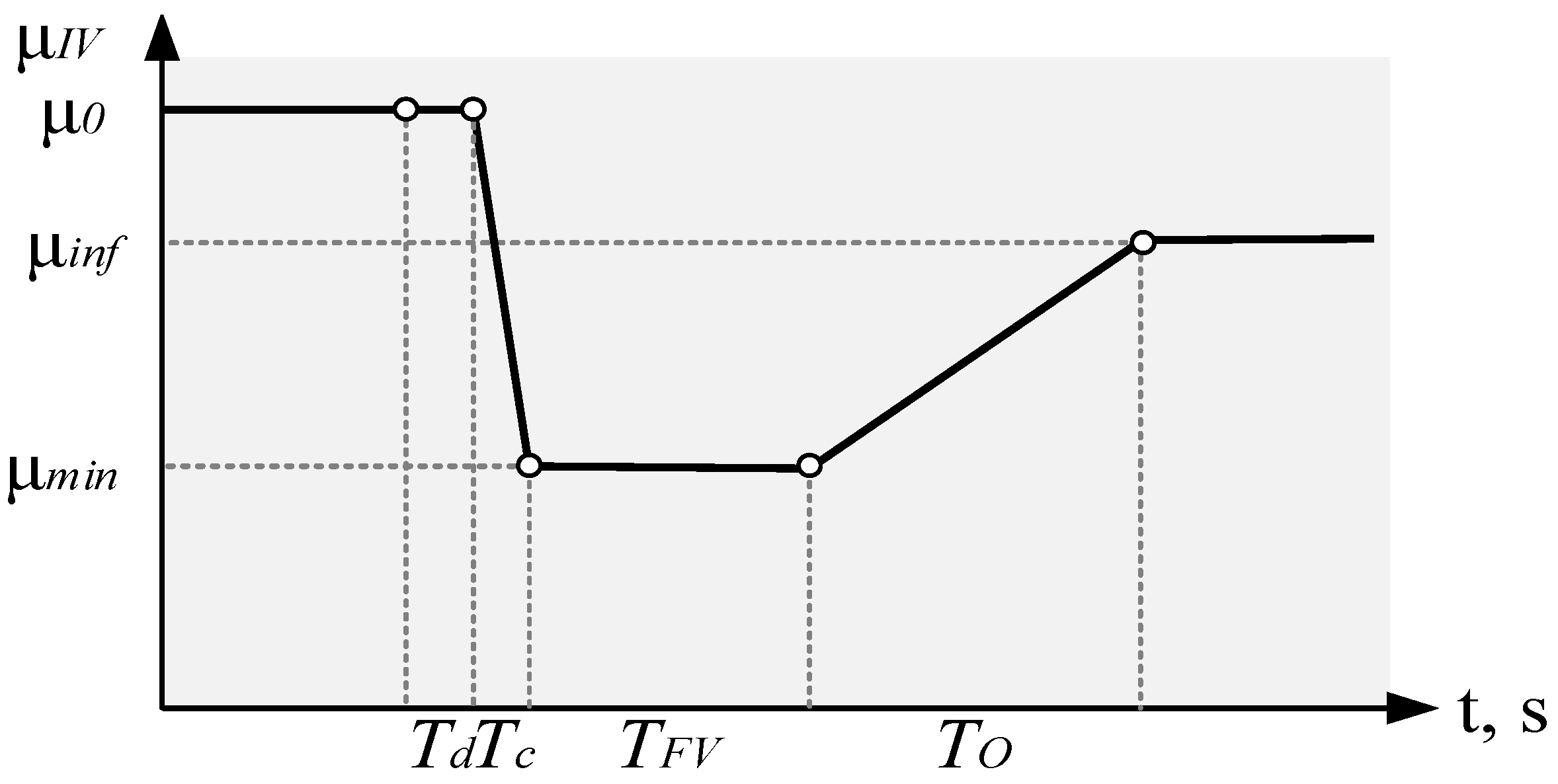
Figure 2 depicts the process of changing IV in the ST FV. The x-axis indicates the time in seconds, the y-axis indicates the position of IV. In particular, Figure 2 shows the following: μ_IV—position IV, μ₀—initial position IV, μ_inf—position IV after ST FV, μ_min—minimum position IV at ST FV, T_d—delay in the start of the IV movement process at ST FV, T_c—closing time IV at ST FV, T_FV—time of holding the minimum position IV at ST FV, and T_o—time of transition from position IV μ_min to position μ_inf.

In determining the characteristics of the IV position change process, the following variables are calculated: μ_inf, μ_min, T_c, T_FV, and T_o. The shut-off valve closes as quickly as possible. To prevent low frequency oscillation (LFO) of the SG active power when the turbine power increases after ST FV, the opening of the shut-off valve is performed at a limited speed [22]. To prevent LFO caused by the actions of the power unit regulators after the ST FV, the IV is opened with a time delay T_o. The time during which the shut-off valve is closed is limited by the technological protections of the steam boiler and individually for each power unit. The depth of turbine ramping and turbine power after ST FV also have limitations due to the permissible operating conditions of the steam boiler and turbine.

Figure 2 shows the following sections of the ST FV process: open position IV, closing process IV, the delay of a closed position IV for the time T_FV, opening the IV for time T_o, and open position IV.

In 1973, R.H. Park published a paper [23] that provides a detailed description of using ST FV to maintain EPS stability. Historically, the initial studies exploring the use of ST FV date back to 1925 [24] and 1928 [25]. Subsequently, the paper [26] highlights the advantages of using ST FV with a delayed opening of the IV:

• The delay when opening IV increases the magnitude of the first swing cycle in the post-emergency operating mode of SG, which increases the probability of maintaining stability;
• When opening IV without delay, the probability of LFO groups of oscillators occurring with a subsequent loss of TS increases.

The study [27] discussed the problem of maintaining superheater pressure when using ST FV. Since the 1980s, active implementation of ST FV began. In the study [28], an expert system was proposed to determine the following parameters of the IV motion in the ST FV process: μ_inf and μ_min. To implement a certain ST FV law in real time, a pre-prepared lookup table was used. However, this approach did not assume sufficient adaptability and considered only a certain set of disturbances for which the values μ_inf and μ_min were prepared in advance. The study did not consider the probability of loss of SG stability in the second and subsequent swing cycles after the implementation of ST FV.

In the study [29], mathematical models of ST in various configurations and methods for modeling ST FV are presented. The effectiveness of ST FV in enhancing EPS sustainability is also demonstrated. The theoretical basis for the effectiveness of ST FV is supported by applying the rule of area (EAC). For numerical modeling, a fragment of the Brazilian EPS consisting of 13 nodes with a voltage class of 345 kV was used. The authors note that the use of ST FV can lead to increased pressure in the ST superheater; therefore, the motion characteristics of the IV should consider the overall technical condition of the superheater. To improve the efficiency and reliability of ST FV, the authors suggest supplementing the ST with a bypass device that diverts part of the steam to the condenser during ST FV implementation.

The authors of [30] propose a technique based on the use of artificial neural networks (ANN) to determine the parameters of the law of IV position change during ST FV. The parameters to be determined were μ_inf, μ_min, and T_FV. The initial power SG, the post-accident power reduction SG, and the rotor acceleration magnitude SG were used as inputs to the ANN algorithm. The general algorithm for using ST FV is as follows: identification of disturbance; within 0.08 s, the input data used for ANN is saved; and the parameters μ_min and T_FV are determined. After 0.65 the parameter μ_inf is determined. Mathematical and physical models were used for testing.

In [31] the ANN algorithm was also used to synthesize the law of IV position change during the ST FV process. The change in active power SG during the disturbance process and the change in rotor speed SG were used as input parameters for the ANN. The output parameters are μ_min, μ_inf, and T_FV. For the numerical experiment, an EPS mathematical model consisting of a 600 MW SG and an IB was used. The performance of the trained ANN algorithm ranged from 60 to 80 ms.

In the study [32] a multi-agent approach (MAS) was used to synthesize the law of IV position change in the ST FV process. The attached algorithm consists of two agents: a tracking agent and a managing agent. The tracking agent models the load angle of each protected SG to track buckling. The control agent determines the values μ_min, μ_inf, and T_FV of the IV position change law during the ST FV process. The input parameters for the developed methodology are pre-emergency active power SG, post-emergency active power SG, and predicted value of the load angle SG. The proposed methodology was tested using mathematical data. The study [33] used the Lyapunov stability theory (LST) to synthesize the ST FV law. To test the methodology, a mathematical model of EPS consisting of three nodes and two SGs was used. The authors of the study [34] used the radial basis function network (RBFNN) algorithm to determine the values of μ_min, μ_inf, and T_FV of the IV position change law during the ST FV process. To determine the required parameters, a system of input and output data similar to [30] was used. The Gaussian function was used as the activation function. The study [35] is devoted to the use of the maximum principle (MP) to synthesize the ST FV law. Testing was performed on a standard IEEE39 model. To synthesize the ST FV law in [36], the transition energy function (TEF) method was used, which is determined by the sum of kinetic and potential energy SG EPS. Testing was performed on the IEEE24 model. In the study [37], the feedback linearization (FL) method was used to select the parameters of the ST FV law. The authors of [38] used the optimization method and the equal area criterion (EAC) with testing on the IEEE 39 model to determine the values of μ_min and T_FV. Also, the direction of studying ST FV contains the following: the analysis of the results of testing on a real-time modeling complex [39], real EPS [40,41], as well as the influence of ST FV on the protection systems of electrical network elements [42].

Table 1. Analysis of considered studies.

Reference	Year of Publication	Algorithm	ST FV Calculated Parameters
[30]	1997	ANN	μmin, μinf, TFV
[31]	1993	ANN	μmin, μinf, TFV
[32]	2002	MAS	μmin, μinf, TFV
[33]	1997	LST	μmin
[34]	1995	RBFNN	μmin, μinf, TFV
[35]	1993	MP	μmin
[36]	2018	TEF	μmin
[37]	2007	FL	μmin
[38]	2021	EAC	μmin, TFV

provides an analysis of the methods considered for synthesizing the ST FV law.

Among the studies reviewed, two groups of methods used to synthesize the optimal ST FV law can be distinguished: ML algorithms and classical algorithms for transient analysis in EPS [43,44,45,46,47].

Today, due to the development of computer technology the availability of large volumes of data on transient processes in EPS and the development of systems for collecting and transmitting information, ML algorithms are actively used for analyzing and managing EPS. Developing and implementing adaptive EPS EC systems based on ML and ST FV becomes possible. Also, for the problem of synthesizing the ST FV law, to use new ML algorithms that eliminate the disadvantages of ANN-based algorithms is possible [48].

3. Methodology

The methodology for introducing ML algorithm into the EPS management process to ensure sustainability can be described as follows:

• Data collection. In this stage, physical or synthetic data obtained during the modeling of transient processes on a mathematical model of the EPS under consideration can be used;
• Data pre-processing. This stage includes the elimination of gaps, noise, and outliers in the data, correlation analysis, processing of features, and identification of the main components in the data;
• Training several ML algorithms to analyze the accuracy, time efficiency, and fault tolerance;
• Testing of algorithms. During this stage the ML algorithm that provides optimal results in terms of accuracy and speed is determined;
• Testing the selected ML algorithm in real time;
• Development and implementation of digital infrastructure that ensures the correct operation of the trained algorithm;
• Monitoring and possible correction of parameters of ML algorithm during use in the EPS control loop.

Figure 3 shows a graphical interpretation of the proposed methodology.

This article covers steps 1–4. The study of steps 5–7 is a task for future research; this work discusses the complete list of stages of the methodology to provide a complete picture of the study.

3.1. Dataset Generation

The data collection stage is a key component when developing an EPS management methodology based on ML algorithms [49]. Sources of input data can include physical changes and synthetic data obtained from modeling a series of transients in EPS. Each data source has its advantages and disadvantages associated with the presence of noise, gaps in the data, inaccuracy in the representation of EPS parameters in the mathematical model, the impossibility of considering the entire list of accidents, etc. [50]. As a result, the most optimal way to generate a data sample is a combination of physical and synthetic data.

When using synthetic data, an important issue is the modeling of changes in the parameters of the EPS electrical mode and the list of considered disturbances. The loads in the nodes are considered as variable parameters when changing the EPS operating mode. Voltages, flows of active and reactive powers, current loads of the electrical network, and SG loads are dependent parameters determined by the requirement to ensure a balance of active power in the EPS. EPS load variations can be modeled considering intra-daily and seasonal variations [51]. In the simplest cases, load changes are modeled using a probabilistic approach.

In this study, a probabilistic approach of load deviation from the base value with a normal distribution was used to model the load change of the test EPS. To obtain the reference laws of IV position change during the ST FV process, the algorithm given in [38] was used. Voltage values at the nodes of the EPS model flow of active and reactive powers across the elements of the electrical network, active and reactive powers of SG, and load angles of SG are used as features.

3.2. Dataset Preparation

One of the key stages of using ML algorithms is collecting and preparing source data. In this study, the results of mathematical modeling were used to generate a data sample. The loads in the nodes of the EPS test model, the node, and the type of simulated disturbance was selected as varied parameters during modeling. The data generation technique used in this article is as follows:

• Formation of a dynamic model of the test EPS in Python3 free software in consideration of the SG parameters, electrical network elements, and loads;
• Specifying a list of accidents to be considered in the form of three-phase, two-phase, and single-phase short circuits (SC) in electrical network nodes;
• For the selected SG, the optimal law of IV variation is calculated to maintain TS;
• The loads in the test EPS nodes are changed by adding a random variable with a normal distribution to the basic load values;
• The calculation of the optimal law of change of IV for maintaining TS is performed;
• A cyclic calculation is performed until the end of the load search in the EPS nodes.

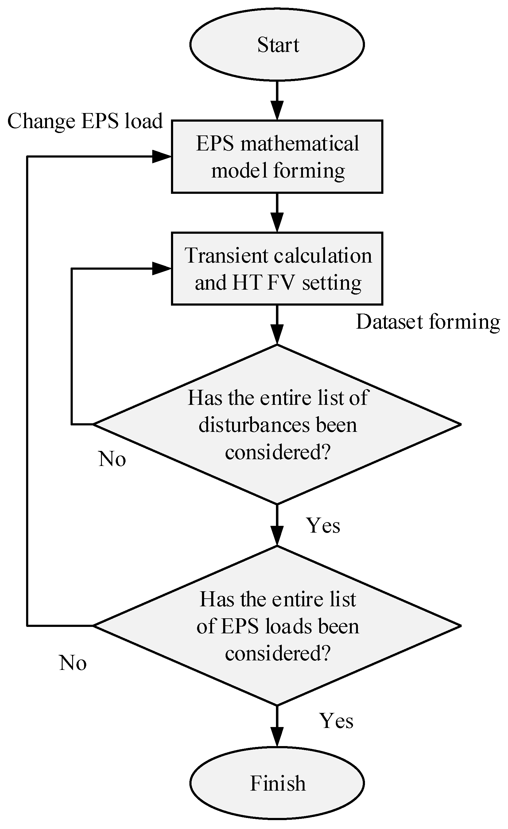
Figure 4 shows a flowchart for generating data samples.

The features in the sample are active and reactive powers SG, load angles SG, flows of active and reactive power through the elements of the electrical network, voltage modules, and phases in the nodes of the electrical network. The target indicator is the law of IV position change in the ST FV process.

3.3. ML Algorithm Selection

The problem of synthesizing the law of IV position change in the ST FV process is a multidimensional classification problem in which various combinations of parameters μ_min, μ_inf, and T_FV act as classes. In this study, the parameters μ_min and T_FV are used to form classes, the value of μ_inf is taken equal to 1.

In this work, to synthesize the ST FV law, classification algorithms were used that are actively used for problems of process analysis in EPS [52]: k-nearest neighbors (KNN), support vector machine (SVM), decision tree (DT), random forest (RF), extreme gradient boosting (XGBoost), and ANN. The choice of these algorithms is determined by a combination of their performance, accuracy, and ease of use. These algorithms are widely used to solve problems in EPS control, analysis, and diagnostics.

The KNN algorithm is one of the simplest classification algorithms, which simply consists of sequentially performing the following operations [53]:

• Calculation of the distance to each of the objects in the training sample;
• Determination of k objects of the training set with the smallest distance;
• Calculate the most frequently encountered class for k objects, which will be the result of the classification.

The algorithm parameter is n_neighbors—the number of objects with a minimum distance. The advantages of the algorithm include resistance to outliers in the data, interpretability of the results, and ease of implementation of the algorithm.

The SVM algorithm [54] uses the technique of constructing a separating hyperplane, which is determined because of training, to classify data. The parameters of the algorithm are C—soft constraint weight, kernel—kernel function, in this work the radial basis function (RBF) kernel is used, and gamma—kernel coefficient. The advantages of the algorithm include a high accuracy, the ability to efficiently process high-dimensional data, and a small number of hyperparameters.

DT [55] is a flexible classification algorithm based on the construction of logical rules. The DT algorithm can be represented as a hierarchical structure, the purpose of which is to split the data sample in order to optimize a pre-determined criterion (Gini coefficient, entropy value, or logistic error function). Training the DT algorithm consists of sequentially performing the following steps:

• Enumerate all the features, and search for the feature with the best separation;
• Dividing the sample into two parts, enumerating the features, and dividing each of the resulting subsamples;
• The division of subsamples continues until subsamples of unit dimension are obtained, which are called DT leaves.

The parameters of the algorithm are as follows: criterion—a function for assessing the quality of data splitting, splitter—a strategy used to select a split at each node, and max_depth—the maximum depth of DT. The advantages of the algorithm include interpretability due to the visual representation capabilities of a trained DT, and efficiency of work on untrained data. As a way to improve the DT algorithm, the RF algorithm [56], which is an ensemble ML algorithm, is used. During the training process of the ensemble algorithm, several DTs are created, which reduces the probability of overfitting.

The classification result of the RF algorithm is an aggregation of the classification of each of the RFs included in the ensemble. Each RF algorithm is trained independently, allowing efficient use of parallel computing. The parameters of the algorithm are as follows: n_estimators—the number of trees in the algorithm, criterion—a function for assessing the quality of data partitioning, and max_depth—the maximum depth of DT. The advantages of the algorithm include a high degree of use of parallel calculations when training and testing the algorithm, high resistance to overtraining, and to assess the importance of each feature for classification.

Further development of the RF algorithm led to the development of the XGBoost algorithm [57]. This algorithm uses gradient boosting to iteratively train weak classifiers. The parameters of the algorithm are as follows: criterion—the function for assessing the quality of data dividing, learning_rate, n_estimators—the number of iterations in boosting, max_depth—the maximum depth of the tree, and max_features—the number of features considered by the algorithm to construct splitting in the tree. The advantages of the algorithm include resistance to overtraining due to the use of L1 and L2 regularizes, a high degree of parallelization, and a high optimization in the use of computing resources.

The following configurable parameters for the ANN algorithm are used: batch_size—the number of records processed together before updating the model parameters, learning_rate—the learning rate, and epochs—the number of epochs. For this study, the ANN is built using a series of fully connected linear layers followed by rectified linear unit (ReLU) activation functions. The input dimension corresponds to the number of features in the processed data set, and the output dimension equals the number of classes in the classification problem.

3.4. ML Algorithm Training and Testing

After generating a data sample, it is processed using statistical analysis methods, a detailed description of which is given in the study [58].

Table 2. Methods for determining hyperparameters of selected ML algorithms.

Algorithm	Training Method	Hyperparameters
KNN	Calculation of distances to classes	[n_neighbors]
SVM	SGD	[C, gamma]
DT	SGD	[max_depth]
RF	SGD	[n_estimators, max_depth]
XGBoost	SGD	[learning_rate, n_estimators, max_depth, max_features]
ANN	SGD	[batch_size, learning_rate, epochs]

summarizes the methods used to determine the hyperparameters in the used ML algorithms. For the SVM, DT, RF and XGBoost algorithms, the main training method is stochastic gradient descent (SGD). For the KNN algorithm, the training is the procedure for calculating the distance between classes.

To estimate the performance of the trained algorithm the following metrics are used: accuracy, precision, recall, F1 score, and the area under the receiver operating characteristic (AUC) [59].

4. Case Study

This section presents the results of generating a data sample for the IEEE39 mathematical model. The calculation of transient processes was performed in a Python3 free software, and the training and testing of the ML algorithms were carried out in a Python 3 program using the scikit-learn and pandas libraries.

4.1. Dataset Generation

To form a data sample, the mathematical model of the IEEE39 EPS test was used [59]. This model is standard for transient studies in EPS and consists of 10 SGs and 39 nodes. The model graphics are shown in Figure 5. The SG parameters are given in

Table 3. SG parameters.

SG	Rated Power, MW	H, s	xd, Ohm	xq, Ohm
1	10,000	5.000	2.00	1.90
2	1000	3.030	2.95	2.82
3	1000	3.580	2.49	2.37
4	1000	2.860	2.62	2.58
5	1000	4.333	4.02	3.72
6	600	3.480	2.54	2.41
7	1000	2.640	2.95	2.92
8	1000	2.430	2.90	2.80
9	1000	3.450	2.10	2.05
10	1000	4.200	1.00	0.69

, and

Table 4. The basic values of loads in the nodes of the EPS test model.

Node	[P; Q], [MW; MVar]	Node	[P; Q], [MW; MVar]
1	[97.6; 44.2]	21	[274; 115]
3	[322; 2.4]	23	[247.5; 84.6]
4	[500; 184]	24	[308.6; 92.2]
7	[233.8; 84]	25	[224; 47.2]
8	[522; 176]	26	[139; 17]
12	[8.5; 88]	27	[281; 75.5]
15	[320; 153]	28	[206; 27.6]
16	[329; 32.3]	29	[283.5; 26.9]
18	[158; 30]	31	[9.2; 4.6]
20	[680; 103]	39	[1104; 250]

shows the base loads at the EPS nodes.

To form a data sample, three-phase, two-phase, and single-phase faults in EPS nodes 1 to 29 were considered. The change in loads in the EPS nodes was performed by adding a random uniformly distributed value to the base loads. Figure 6 shows the load distributions in the nodes of the IEEE39 model. The ordinate axes show the numbers of nodes with loads and the abscissa shows the active powers of the loads.

The total volume of the data sample was 300 transient processes, for which one of six classes was selected, describing the laws of IV position change in the ST FV process. The considered laws of change in the IV position are described by the following combinations:

$$Class\left({\mathsf{\mu }}_{min},T_{FV}\right)=\left[\begin{array}{c}Class1\\ Class2\\ Class3\\ Class4\\ Class5\\ Class6\end{array}\right]=\left[\begin{array}{c}\begin{array}{cc}0.2& 0.1\end{array}\\ \begin{array}{cc}0.2& 0.2\end{array}\\ \begin{array}{cc}0.4& 0.1\end{array}\\ \begin{array}{cc}0.4& 0.2\end{array}\\ \begin{array}{cc}0.6& 0.1\end{array}\\ \begin{array}{cc}0.6& 0.2\end{array}\end{array}\right].$$

(1)

Table 5. The description of features in the data sample.

№	Feature Set	Feature Number
1	Voltages at EPS nodes during SC	[1:38]
2	SG active powers during SC	[39:47]
3	SG reactive powers during SC	[48:56]
4	Active power flows under SC	[57:103]
5	Reactive power flows under SC	[104:149]
6	Current loads of network elements during SC	[150:196]

provides a description of the of the data sample features.

For a more visual representation of the training set, Figure 7 shows a graph of the distribution of classes in the sample from the first (PC₁) and second (PC₂) principal components of the data [60].

Figure 7 illustrates the clustering of data between the six considered classes of the IV position change law during the ST FV process.

4.2. Feature Selection

A two-step procedure was used to select significant features in the generated data sample [61]:

• Analysis of the Spearman correlation coefficient of each feature related to the class;
• Analysis of the mutual Spearman correlation coefficient between features.

Table 6. Results of feature selection.

Feature Set Number	Feature Number	Analyses Step	Removed
1	[1:38]	(1)	[5:12, 24]
2	[39:47]		[—]
3	[48:56]		[49, 51:53]
4	[57:103]		[68:73, 88:96]
5	[104:149]		[107:121]
6	[150:196]		[150:188]
1	[1:30]	(2)	[2, 4]
2	[31:39]		[—]
3	[40:45]		[41, 44]
4	[46:79]		[62, 73]
5	[80:111]		[90, 105]
6	[112:120]		[115, 123, 128]

shows the feature selection results. When analyzing the Spearman correlation coefficient of each feature concerning the class, features with a correlation coefficient value below 0.4 were removed. When analyzing the mutual correlation coefficient between features, features with a correlation coefficient value higher than 0.8 were removed.

The following designations are used in Table 6: “Feature set number” corresponds to the “№” column in Table 5, and “Analyzes step” corresponds to the step of the feature selection procedure. After deletion, the individual features are renumbered. The “—” symbol in the “Removed features” column indicates the absence of features to be removed.

During the analysis of features in the data sample, in the first stage of processing, 76 features were removed, and the largest number of features were removed from the group of features of current loads of electrical network elements. In the second stage of feature selection, 11 features were removed.

4.3. Algorithms Training and Testing

To train and test the selected ML algorithms, the data sample was divided into training and testing with a ratio of 80/20.

Figure 8 shows the dependence of the accuracy coefficient on the n_neighbors parameter in the training and test selections of the KNN algorithm. Figure 9 shows the dependence of the accuracy coefficient on the epoch parameter in the training and test selections of the DT algorithm. Figure 10 shows the dependence of the accuracy coefficient on the epoch parameter in the training and test selections of the RF algorithm.

Table 7. Quality metrics of the considered algorithms in the training data sample.

Algorithm	Accuracy, %	Precision, %	Recall, %	F1 Score, %	AUC, %
KNN	95.18	88.42	81.17	84.64	81.12
SVM	93.15	84.17	83.49	83.82	80.54
DT	85.93	70.22	68.91	69.55	78.14
RF	94.31	88.06	84.18	86.07	82.58
XGBoost	98.17	90.43	88.12	89.26	88.48
ANN	96.97	93.12	95.44	94.26	95.12

shows the quality metrics of the considered ML algorithms in the training data set.

Table 8. Quality metrics of the considered algorithms in the test data sample.

Algorithm	Accuracy, %	Precision, %	Recall, %	F1 Score, %	AUC, %
KNN	94.21	87.12	83.71	85.38	82.45
SVM	89.45	86.14	82.17	84.10	81.73
DT	82.15	71.14	68.12	69.59	79.47
RF	93.62	87.11	86.49	86.79	84.79
XGBoost	97.14	91.12	89.14	90.11	91.48
ANN	96.21	95.34	98.21	96.75	97.14

shows the quality metrics of the considered ML algorithms on the test data set.

Table 9. Methods for determining hyperparameters of selected ML algorithms.

Algorithm	Hyperparameters
KNN	n_neighbors = 15
SVM	C = 4, gamma = 0.03
DT	max_depth = 16
RF	n_estimators = 14, max_depth = 12
XGBoost	learning_rate = 0.2, n_estimators = 12, max_depth = 8, max_features = 10
ANN	batch_size = 30, learning_rate = 0.001, epochs = 200

shows the obtained values of the hyperparameters of the considered ML algorithms.

One of the main parameters in the EPS EC algorithm is performance, which is expressed in the time delay required to select the optimal CA value to ensure TS or SSS. In the algorithm presented in [38], the delay value of the algorithm was 200 ms, which makes it possible to use it for SGs with a constant inertia value of 2.5 s.

Table 10. Time delays of the considered ML algorithms.

Algorithm	One Class Classification (Training), ms	One Class Classification (Testing), ms
KNN	16.2	12.3
SVM	15.8	14.2
DT	12.5	11.4
RF	10.3	8.7
XGBoost	4.2	3.8
ANN	6.7	5.2

shows the results of determining the delay in the considered ML algorithms when determining the CA value for one transient process. Calculations were performed on a computer with an Intel (R) Core (TM) i7-7700T CPU @ 2.90 GHz, 16 GB of RAM.

The use of ML algorithms can significantly increase the speed of selecting the optimal CA for saving EPS TS or SSS. The largest time delay corresponds to the KNN algorithm, which is explained by the need to store the entire volume of the training sample in the computer’s RAM. The minimum time delay on the test and training set corresponds to the XGBoost algorithm. Also, the highest classification accuracy corresponds to the XGBoost algorithm.

5. Conclusions

The development of modern EPS significantly impacts the accuracy and adaptability of EPS EC algorithms. With the introduction of a considerable amount of RES, the nature of the transition processes in EPS is undergoing radical changes. An increase in the speed of transient processes, along with a rise in the stochasticity of EPS operation, necessitates a revision of the operating principles in EPS EC devices. The advantages of the proposed method include high adaptability and performance. One of the difficulties of the technique is the process of matting the data sample and re-training the model when the configuration in the protected EPS is changed. However, this feature can be mitigated by developing an automatic approach for generating data during the operation of the EPS.

The problem of implementing an adaptive selection of the ST FV law based on an ML algorithm has been considered in the study. To form a data sample, the EPS IEEE39 mathematical model was used. A total of 300 transient processes were considered, of which 196 features were identified. After statistical analysis, the number of features was reduced to 109.

Next, the procedures for training and testing the KNN, SVM, DT, RF, XGBoost, and ANN algorithms were performed on the generated data samples. The highest accuracy on the training and test samples corresponds to the XGBoost algorithm (98.17% on the training set and 97.14% on the test set). The smallest computational delay for classifying one transient process also corresponds to the XGBoost algorithm (4.2 ms on the training set and 3.8 ms on the test set).

The following can be considered as directions for further research on the topics discussed in this article: development of a methodology for selecting CAs based on ML algorithms for storing TS and SSS in combined EPS; CA selection based on ML algorithms to maintain voltage stability and maintain a required frequency level; testing the developed methods on a real-time modeling complex; and development of an architecture for implementing the ESP EC methodology based on ML algorithms in the operational control loop of an EPS operation.

References

1. Li, X.; Gao, L.; Wang, G.; Gao, F.; Wu, Q. Investing and pricing with supply uncertainty in electricity market: A general view combining wholesale and retail market. China Commun. 2015, 12, 20–34. [Google Scholar] [CrossRef]
2. Ayuyev, B.I.; Yerokhin, P.M.; Shubin, N.G.; Neujmin, V.G.; Mashalov, E.V. The software complex of optimal power flow solution for united power system of Russia in a terms of competitive electricity market. In Proceedings of the 2005 IEEE Russia Power Tech, St. Petersburg, Russia, 27–30 June 2005; pp. 1–5. [Google Scholar] [CrossRef]
3. Ge, X.; Qian, J.; Fu, Y.; Lee, W.-J.; Mi, Y. Transient Stability Evaluation Criterion of Multi-Wind Farms Integrated Power System. IEEE Trans. Power Syst. 2022, 37, 3137–3140. [Google Scholar] [CrossRef]
4. Tu, J.; Zhou, M.; Cui, H.; Li, F. An Equivalent Aggregated Model of Large-Scale Flexible Loads for Load Scheduling. IEEE Access 2019, 7, 143431–143444. [Google Scholar] [CrossRef]
5. XUE, Y.; ZHU, X.; LI, Z. Influence of Generator-tripping Time on Transient Stability. In Proceedings of the 2019 IEEE Innovative Smart Grid Technologies—Asia (ISGT Asia), Chengdu, China, 21–24 May 2019; pp. 916–921. [Google Scholar] [CrossRef]
6. Ruban, N.; Kievets, A.; Andreev, M.; Suvorov, A. Turbine Fast Valving Setting Method Based on the Hybrid Simulation Approach. Energies 2023, 16, 1745. [Google Scholar] [CrossRef]
7. Alqahtani, S.; Shaher, A.; Garada, A.; Cipcigan, L. Frequency Stability in Renewable-Rich Modern Power Systems, Saudi Grid Case Study. In Proceedings of the 2022 57th International Universities Power Engineering Conference (UPEC), Istanbul, Turkey, 30 August–2 September 2022; pp. 1–6. [Google Scholar] [CrossRef]
8. Shi, Z.; Wang, W.; Huang, Y.; Li, P.; Dong, L. Simultaneous optimization of renewable energy and energy storage capacity with the hierarchical control. CSEE J. Power Energy Syst. 2022, 8, 95–104. [Google Scholar] [CrossRef]
9. Mai, T.; Hand, M.M.; Baldwin, S.F.; Wiser, R.H.; Brinkman, G.L.; Denholm, P.; Arent, D.J.; Porro, G.; Sandor, D.; Hostick, D.J.; et al. Renewable Electricity Futures for the United States. IEEE Trans. Sustain. Energy 2014, 5, 372–378. [Google Scholar] [CrossRef]
10. Elavarasan, R.M.; Shafiullah, G.M.; Padmanaban, S.; Kumar, N.M.; Annam, A.; Vetrichelvan, A.M.; Mihet-Popa, L.; Holm-Nielsen, J.B. A Comprehensive Review on Renewable Energy Development, Challenges, and Policies of Leading Indian States with an International Perspective. IEEE Access 2020, 8, 74432–74457. [Google Scholar] [CrossRef]
11. Ghosh, S.; Isbeih, Y.J.; Azman, S.K.; Moursi, M.S.E.; El-Saadany, E. Optimal PMU Allocation Strategy for Completely Observable Networks with Enhanced Transient Stability Characteristics. IEEE Trans. Power Deliv. 2022, 37, 4086–4102. [Google Scholar] [CrossRef]
12. Wang, X.; Shi, D.; Wang, J.; Yu, Z.; Wang, Z. Online Identification and Data Recovery for PMU Data Manipulation Attack. IEEE Trans. Smart Grid 2019, 10, 5889–5898. [Google Scholar] [CrossRef]
13. Beryozkina, S.; Senyuk, M.; Berdin, A.; Dmitrieva, A.; Dmitriev, S.; Erokhin, P. The Accelerate Estimation Method of Power System Parameters in Static and Dynamic Processes. IEEE Access 2022, 10, 61522–61529. [Google Scholar] [CrossRef]
14. Smolovik, S.V.; Koshcheev, L.A.; Lisitsyn, A.A.; Denisenko, A.I. Special Automation for Isolated Power Systems Emergency Control. In Proceedings of the 2021 IEEE Conference of Russian Young Researchers in Electrical and Electronic Engineering (ElConRus), St. Petersburg, Moscow, Russia, 26–29 January 2021; pp. 1558–1561. [Google Scholar] [CrossRef]
15. Senyuk, M.; Odinaev, I.; Pichugova, O.; Ahyoev, J. Methodology for Forming a Training Sample for Power Systems Emergency Control Algorithm Based on Machine Learning. In Proceedings of the 2023 Belarusian-Ural-Siberian Smart Energy Conference (BUSSEC), Ekaterinburg, Russia, 25–29 September 2023; pp. 54–59. [Google Scholar] [CrossRef]
16. Khalyasmaa, A.I.; Senyuk, M.D.; Eroshenko, S.A. Analysis of the State of High-Voltage Current Transformers Based on Gradient Boosting on Decision Trees. IEEE Trans. Power Deliv. 2021, 36, 2154–2163. [Google Scholar] [CrossRef]
17. Khalyasmaa, A.I.; Senyuk, M.D.; Eroshenko, S.A. High-Voltage Circuit Breakers Technical State Patterns Recognition Based on Machine Learning Methods. IEEE Trans. Power Deliv. 2019, 34, 1747–1756. [Google Scholar] [CrossRef]
18. Khalyasmaa, A.I.; Senyuk, M.D.; Eroshenko, S.A. Training sample formation for intelligent recognition of circuit breakers states patterns. In Proceedings of the 2018 IEEE 59th International Scientific Conference on Power and Electrical Engineering of Riga Technical University (RTUCON), Riga, Latvia, 12–14 November 2018; pp. 1–6. [Google Scholar] [CrossRef]
19. Kundur, P.; Klein, M.; Rogers, G.J.; Zywno, M.S. Application of power system stabilizers for enhancement of overall system stability. IEEE Trans. Power Syst. 1989, 4, 614–626. [Google Scholar] [CrossRef]
20. Pavella, M. Generalized one-machine equivalents in transient stability studies. IEEE Power Eng. Rev. 1998, 18, 50–52. [Google Scholar] [CrossRef]
21. Kundur, P. Power System Stability and Control; McGraw-Hill, Inc.: New York, NY, USA, 1994. [Google Scholar]
22. Senyuk, M.; Elnaggar, M.F.; Safaraliev, M.; Kamalov, F.; Kamel, S. Statistical Method of Low Frequency Oscillations Analysis in Power Systems Based on Phasor Measurements. Mathematics 2023, 11, 393. [Google Scholar] [CrossRef]
23. Park, R.H. Fast Turbine Valving. IEEE Trans. Power Appar. Syst. 1973, PAS-92, 1065–1073. [Google Scholar] [CrossRef]
24. Dougherty, J.J.; Monteith, A.C.; Hayward, A.P.; Griscom, S.B. Power system governing—The problem. Electr. Eng. 1941, 60, 547–558. [Google Scholar] [CrossRef]
25. Staege, S.A. Regulator System. U.S. Patent No. 1,705,688, 19 March 1929. [Google Scholar]
26. Cushing, E.W., Jr.; Drechsler, G.E.; Killgoar, W.P.; Marshall, H.G.; Stewart, H.R. Fast valving as an aid to power system transient stability and prompt resynchronization and rapid reload after full load rejection. IEEE Trans. Power Appar. Syst. 1972, 4, 1624–1636. [Google Scholar] [CrossRef]
27. Sullivan, A.C.; Evans, F.J. Some model experiments in fast valving to improve transient stability. In IEEE Transactions on Power Apparatus and Systems; IEEE Paper C 72 242-1; IEEE-INST Electrical Electronics Engineers Inc.: New York, NY, USA, 1972. [Google Scholar]
28. Sun, G.; Lin, W.; Yang, J. Technical Manual of the Control Unit (Model SSC) for Power System Stability Applied in Beilun Port Power Station; Internal Report; Nanjing Institute of Automation: Nanjing, China, 1990. [Google Scholar]
29. Prioste, F.B.; Mendes, P.P.C.; Ferreira, C. Power system transient stability enhancement by fast valving. In Proceedings of the 2004 IEEE/PES Transmision and Distribution Conference and Exposition: Latin America (IEEE Cat. No. 04EX956), Sao Paulo, Brazil, 8–11 November 2004; pp. 639–644. [Google Scholar] [CrossRef]
30. Han, Y.; Xiu, L.; Wang, Z.; Chen, Q.; Tan, S. Artificial neural networks controlled fast valving in a power generation plant. IEEE Trans. Neural Netw. 1997, 8, 373–389. [Google Scholar] [CrossRef] [PubMed]
31. Yong, M.; Wei, J.; Qirong, J.; Han, Y.; Zhou, J. Coordinative control of excitation and fast valving using artificial neural networks. In Proceedings of the TENCON ‘93, IEEE Region 10 International Conference on Computers, Communications and Automation, Beijing, China, 19–21 October 1993; Volume 5, pp. 14–18. [Google Scholar] [CrossRef]
32. Karady, G.G.; Mohamed, M.A. Improving transient stability using fast valving based on tracking rotor-angle and active power. In Proceedings of the IEEE Power Engineering Society Summer Meeting, Chicago, IL, USA, 21–25 July 2002; Volume 3, pp. 1576–1581. [Google Scholar] [CrossRef]
33. Liu, G.X.; Lin, X.S.; Yang, Q.X.; Lai, L.L.; Hogg, B.W. Investigation of turbine valving control with Lyapunov theory. In Proceedings of the 1997 Fourth International Conference on Advances in Power System Control, Operation and Management, APSCOM-97. (Conf. Publ. No. 450), Hong Kong, 11–14 November 1997; Volume 2, pp. 505–508. [Google Scholar] [CrossRef]
34. Chen, Q.; Tan, S.; Han, Y.; Wang, Z. Fast valving control using radial-basis function neural network. In Proceedings of the ICNN’95—International Conference on Neural Networks, Perth, WA, Australia, 27 November–1 December 1995; Volume 5, pp. 2247–2251. [Google Scholar] [CrossRef]
35. Quanxi, C.; Daren, Y.; Songhai, Y.; Zhuo, L. An optimal control method for fast valving using maximum principle. In Proceedings of the TENCON ’93: IEEE Region 10 International Conference on Computers, Communications and Automation, Beijing, China, 19–21 October 1993; Volume 4, pp. 155–157. [Google Scholar] [CrossRef]
36. Vaiman, M.; Vaiman, M. Stability Analysis and Control of Power Systems with Sustained Fast Turbine Valving and Generator Tripping. In Proceedings of the 2018 IEEE Power & Energy Society General Meeting (PESGM), Portland, OR, USA, 5–9 August 2018; pp. 1–5. [Google Scholar] [CrossRef]
37. Anene, E.C.; Aliyu, U.O.; Levine, J.; Venayagamoorthy, G.K. Flatness-Based Feedback Linearization of A Synchronous Machine Model With Static Excitation And Fast Turbine Valving. In Proceedings of the 2007 IEEE Power Engineering Society General Meeting, Tampa, FL, USA, 24–28 June 2007; pp. 1–6. [Google Scholar] [CrossRef]
38. Senyuk, M.D.; Moiseichenkov, A.N.; Kovalenko, P.Y.; Dmitrieva, A.A. Adaptive Algorithm for Steam Turbine Fast Valving Based on the Equal Area Criterion and Synchrophasor Measurements. In Proceedings of the 2021 International Conference on Electrotechnical Complexes and Systems (ICOECS), Ufa, Russia, 16–18 November 2021; pp. 68–73. [Google Scholar] [CrossRef]
39. Kielian, M.; Lis, R. Turbine Fast Valving Study by the Use of a Steam Turbine Real-Time Simulator. In Proceedings of the 2018 22nd International Conference Electronics, Palanga, Lithuania, 18–20 June 2018; pp. 1–5. [Google Scholar] [CrossRef]
40. Bhatt, N.B. Field experience with momentary fast turbine valving and other special stability controls employed at AEP’s Rockport plant. IEEE Trans. Power Syst. 1996, 11, 155–161. [Google Scholar] [CrossRef]
41. Pasternack, B.M.; Bhatt, N.B. The Rockport plant-analysis of temporary fast turbine valving tests. IEEE Trans. Power Syst. 1988, 3, 529–540. [Google Scholar] [CrossRef]
42. Delfino, B.; Denegri, G.B.; Pinceti, P.; Marconato, R.; Scarpellini, P. Impact of turbine fast-valving on generator and transformer protective relays. In Proceedings of the Joint International Power Conference Athens Power Tech, Athens, Greece, 5–8 September 1993; pp. 727–731. [Google Scholar] [CrossRef]
43. Tian, J.; Zhu, J.; Wu, C.; Pan, Z. An Electronic Transformer Fault Identification Method Based on IPOA-DBN. In Proceedings of the 2023 2nd Asia Power and Electrical Technology Conference (APET), Shanghai, China, 17–19 November 2023; pp. 244–247. [Google Scholar] [CrossRef]
44. Senyuk, M.; Safaraliev, M.; Kamalov, F.; Sulieman, H. Power System Transient Stability Assessment Based on Machine Learning Algorithms and Grid Topology. Mathematics 2023, 11, 525. [Google Scholar] [CrossRef]
45. Huy, T.H.B.; Vo, D.N.; Nguyen, H.D.; Truong, H.P.; Dang, K.T.; Truong, K.H. Enhanced Power System State Estimation Using Machine Learning Algorithms. In Proceedings of the 2023 International Conference on System Science and Engineering (ICSSE), Ho Chi Minh, Vietnam, 27–28 July 2023; pp. 401–405. [Google Scholar] [CrossRef]
46. Rao, T.S.M.; Anuradha, T.; Kaur, U.; Rajan, M.S.; Patnala, T.R.; Kumar, V.R. Machine Learning for the Assessment of Transient Stability of Power Systems. In Proceedings of the 2022 6th International Conference on Intelligent Computing and Control Systems (ICICCS), Madurai, India, 25–27 May 2022; pp. 1238–1242. [Google Scholar] [CrossRef]
47. Reyes, A.; Salgueiro, Y.; Rivera, M.; Camargo, J.; Hernández, A.; Wheeler, P. Critical scenarios identification in power system simulations using graph measures and machine learning. In Proceedings of the 2021 IEEE CHILEAN Conference on Electrical, Electronics Engineering, Information and Communication Technologies (CHILECON), Valparaíso, Chile, 6–9 December 2021; pp. 1–6. [Google Scholar] [CrossRef]
48. Abdolrasol, M.G.M.; Hussain, S.M.S.; Ustun, T.S.; Sarker, M.R.; Hannan, M.A.; Mohamed, R.; Ali, J.A.; Mekhilef, S.; Milad, A. Artificial Neural Networks Based Optimization Techniques: A Review. Electronics 2021, 10, 2689. [Google Scholar] [CrossRef]
49. Alzahrani, S.; Shah, R.; Mithulananthan, N. Exploring the Dynamic Voltage Signature of Renewable Rich Weak Power System. IEEE Access 2020, 8, 216529–216542. [Google Scholar] [CrossRef]
50. Senyuk, M.; Safaraliev, M.; Pazderin, A.; Pichugova, O.; Zicmane, I.; Beryozkina, S. Methodology for Power Systems’ Emergency Control Based on Deep Learning and Synchronized Measurements. Mathematics 2023, 11, 4667. [Google Scholar] [CrossRef]
51. Son, J.; Cha, J.; Kim, H.; Wi, Y.-M. Day-Ahead Short-Term Load Forecasting for Holidays Based on Modification of Similar Days’ Load Profiles. IEEE Access 2022, 10, 17864–17880. [Google Scholar] [CrossRef]
52. Alimi, O.A.; Ouahada, K.; Abu-Mahfouz, A.M. A Review of Machine Learning Approaches to Power System Security and Stability. IEEE Access 2020, 8, 113512–113531. [Google Scholar] [CrossRef]
53. Samet, H. K-Nearest Neighbor Finding Using MaxNearestDist. IEEE Trans. Pattern Anal. Mach. Intell. 2008, 30, 243–252. [Google Scholar] [CrossRef] [PubMed]
54. Ding, W.; Tong, Y.; Zhang, Q.; Yang, D. Image and video quality assessment using neural network and SVM. Tsinghua Sci. Technol. 2008, 13, 112–116. [Google Scholar] [CrossRef]
55. Li, Y.; Dong, M.; Kothari, R. Classifiability-based omnivariate decision trees. IEEE Trans. Neural Netw. 2005, 16, 1547–1560. [Google Scholar] [CrossRef]
56. Deng, W.; Guo, Y.; Liu, J.; Li, Y.; Liu, D.; Zhu, L. A missing power data filling method based on improved random forest algorithm. Chin. J. Electr. Eng. 2019, 5, 33–39. [Google Scholar] [CrossRef]
57. Li, N.; Li, B.; Gao, L. Transient Stability Assessment of Power System Based on XGBoost and Factorization Machine. IEEE Access 2020, 8, 28403–28414. [Google Scholar] [CrossRef]
58. Tan, B.; Yang, J.; Tang, Y.; Jiang, S.; Xie, P.; Yuan, W. A Deep Imbalanced Learning Framework for Transient Stability Assessment of Power System. IEEE Access 2019, 7, 81759–81769. [Google Scholar] [CrossRef]
59. Zhang, X.; Chen, Y.; Wang, Y.; Ding, R.; Zheng, Y.; Wang, Y.; Zha, X.; Cheng, X. Reactive Voltage Partitioning Method for the Power Grid with Comprehensive Consideration of Wind Power Fluctuation and Uncertainty. IEEE Access 2020, 8, 124514–124525. [Google Scholar] [CrossRef]
60. Deng, X.; Tian, X.; Chen, S.; Harris, C.J. Nonlinear Process Fault Diagnosis Based on Serial Principal Component Analysis. IEEE Trans. Neural Netw. Learn. Syst. 2018, 29, 560–572. [Google Scholar] [CrossRef]
61. Islam, M.R.; Lima, A.A.; Das, S.C.; Mridha, M.F.; Prodeep, A.R.; Watanobe, Y. A Comprehensive Survey on the Process, Methods, Evaluation, and Challenges of Feature Selection. IEEE Access 2022, 10, 99595–99632. [Google Scholar] [CrossRef]
Figure 1. Electric power generation unit scheme.
Mathematics 12 01644 g001
Figure 2. IV position change graph.
Mathematics 12 01644 g002
Figure 3. Proposed mythology flowchart.
Mathematics 12 01644 g003
Figure 4. Dataset preparation flowchart.
Mathematics 12 01644 g004
Figure 5. IEEE39 test system.
Mathematics 12 01644 g005
Figure 6. The graphs of load distributions in the nodes of the IEEE39 model.
Mathematics 12 01644 g006
Figure 7. Principal component dataset analyses.
Mathematics 12 01644 g007
Figure 8. Changing the value of the accuracy coefficient for the KNN algorithm in training and test samples.
Mathematics 12 01644 g008
Figure 9. Changing the value of the accuracy coefficient for the DT algorithm in training and test samples.
Mathematics 12 01644 g009
Figure 10. Changing the value of the accuracy coefficient for the RF algorithm in training and test samples.
Mathematics 12 01644 g010