


A Composite Half-Normal-Pareto Distribution with Applications to Income and Expenditure Data


Abstract
1. Introduction
2. CHNP Distribution
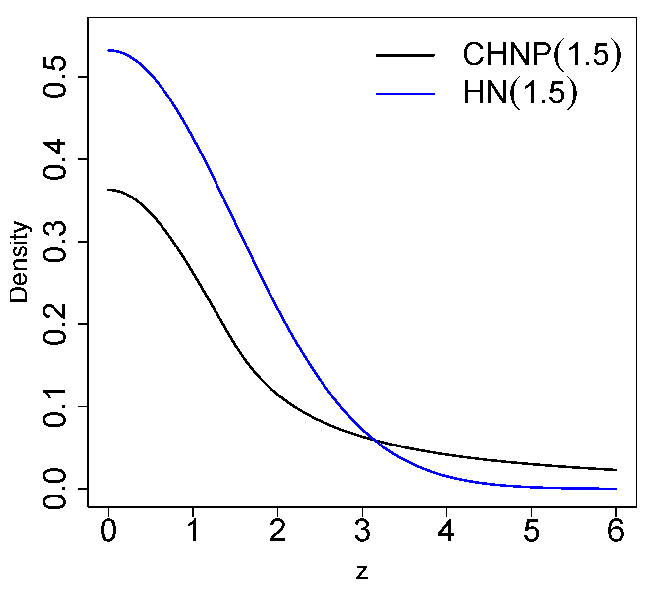
2.1. Density Function
2.2. Properties
- 1.
- The survival function , which is the probability that an article will not fail before time t, is defined by . The survival function for a random variable is given by
- 2.
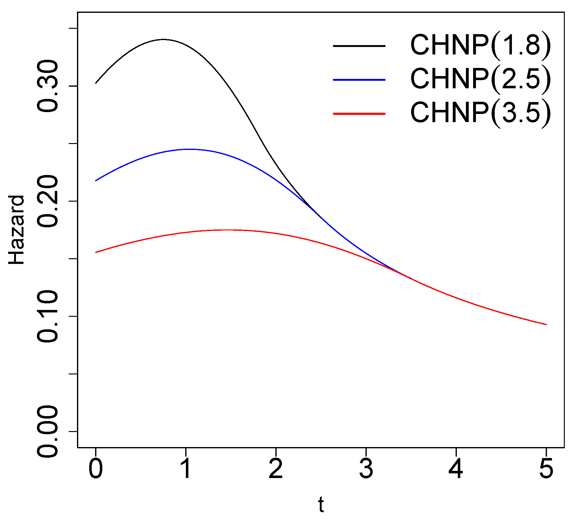
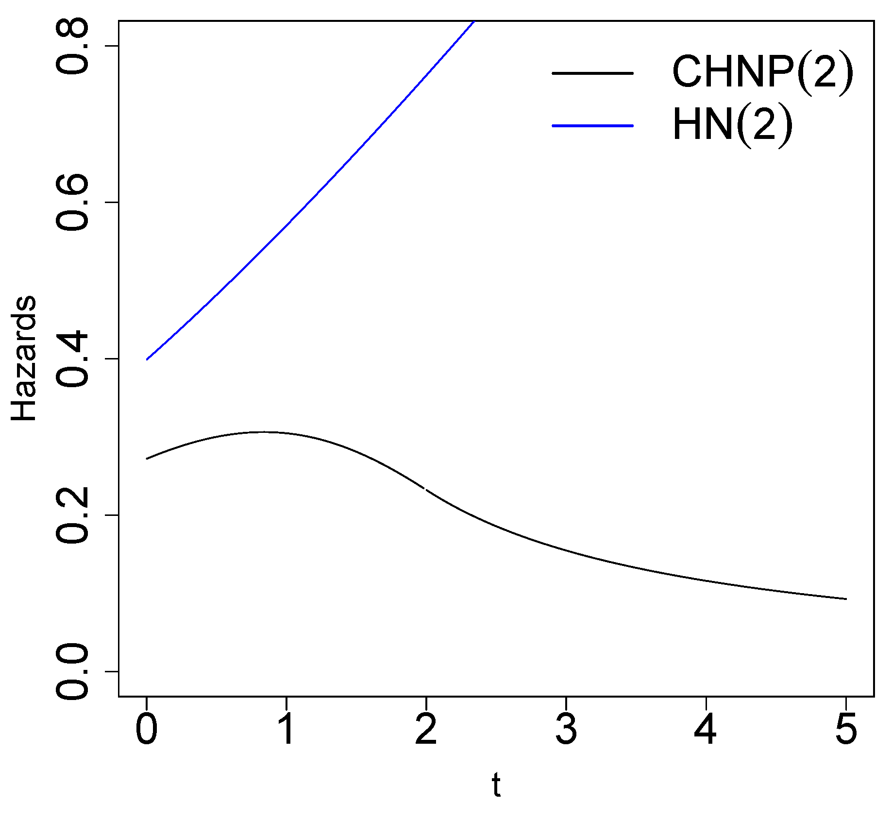
- The hazards function , defined by , for a random variable, is given by
Right Tail of the CHNP Distribution
| Algorithm 1 The algorithm for simulating from the can proceed as follows |
|
- 1:
- Generate
- 2:
- 3:
- Compute
2.3. Actuarial Measure
3. Parameter Estimation
3.1. A Method Based on Percentiles
3.2. ML Estimation
- (i)
- ,
- (ii)
- ,
3.3. Simulation Study
4. Applications
4.1. Numerical Application
- A method based on percentiles. For this example, . We have and . Thus, the estimator of is , where and .
- ML estimation. Using the value of found with the previous method, we calculate the estimator given in Equation (8). This gives us . We observe that the ratio is not satisfied. Therefore, we must use another value for m, for example ; with this, we obtain , and now we observe that the ratio is satisfied, where and . Thus, the ML estimate of is .
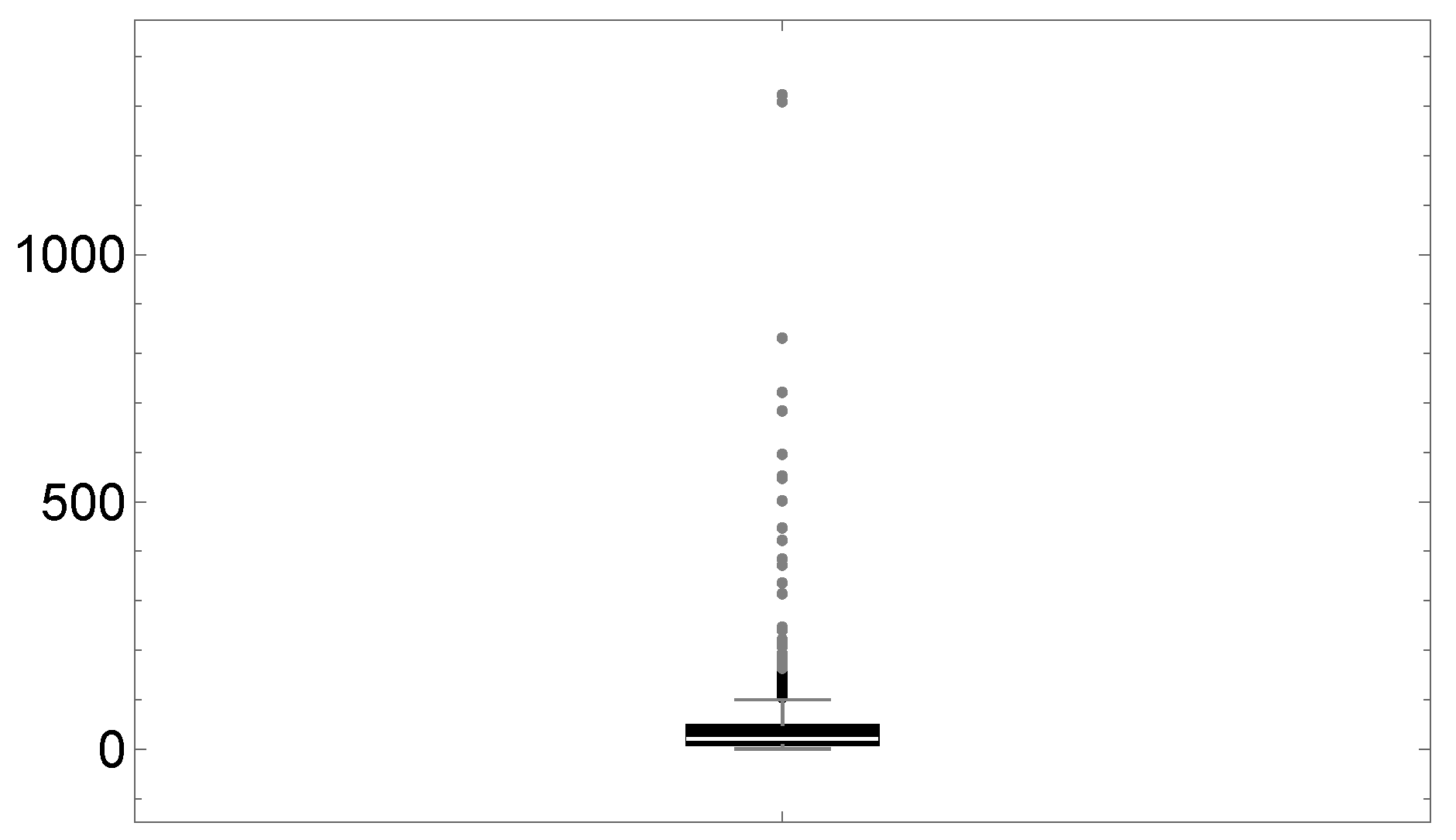
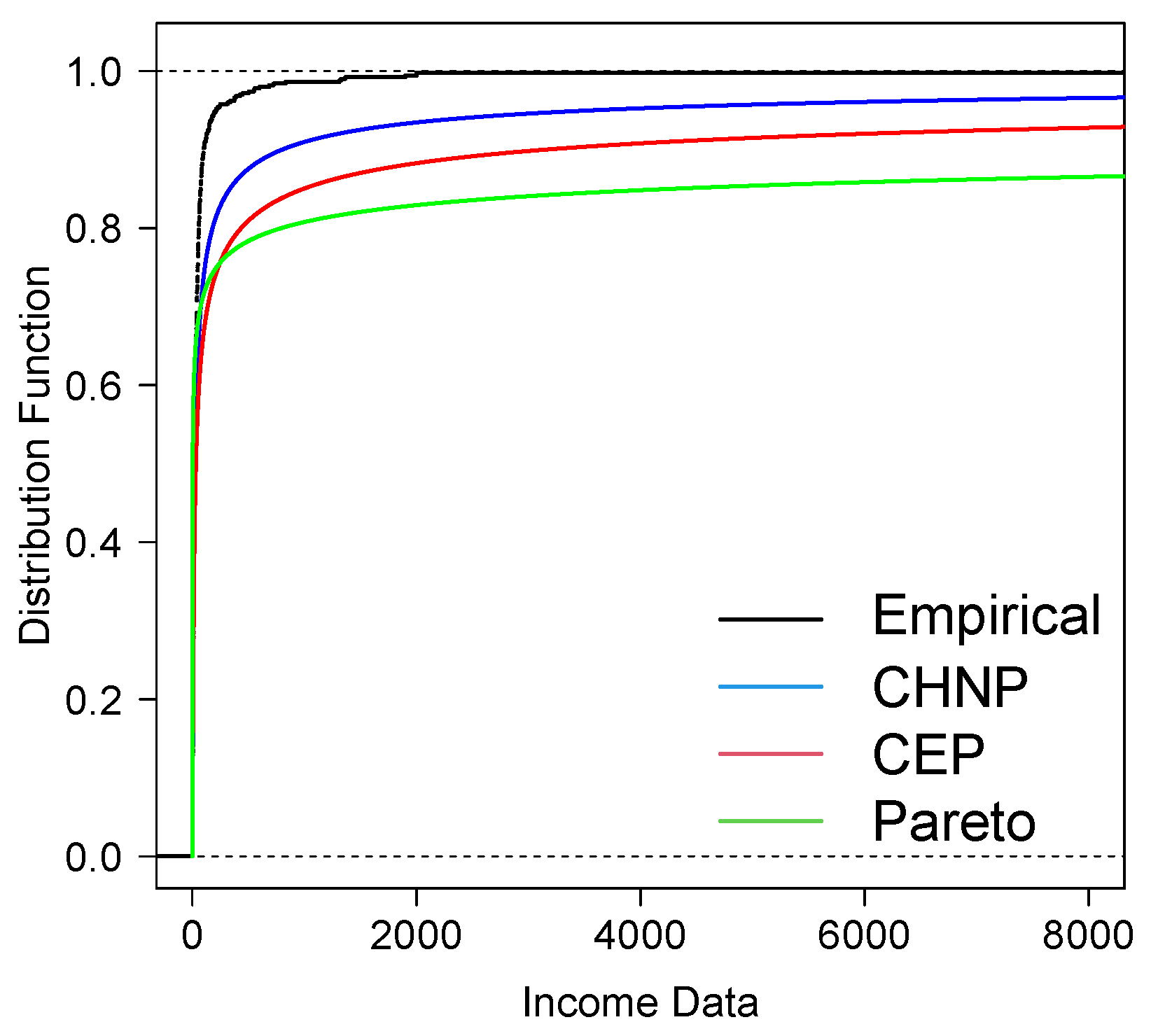
4.2. Application to Income Data
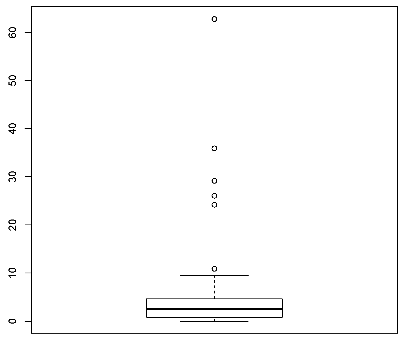
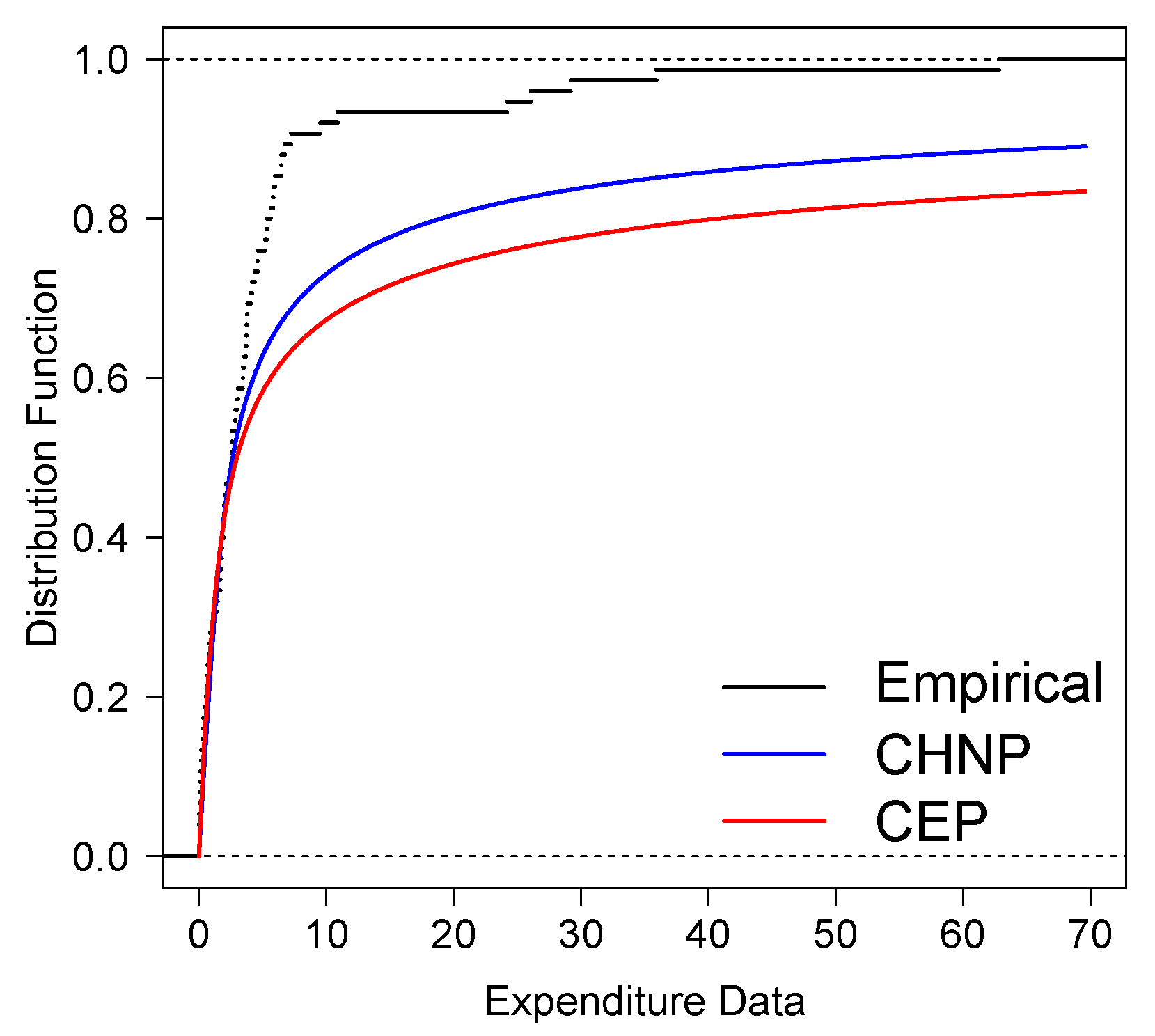
4.3. Application to Expenditure Data
5. Concluding Remarks
- The CHNP model has a heavy right tail, as is shown by Proposition 4.
- The support of the CHNP model contains zero. It is a property that is very important for modeling datasets containing zero.
- Cdf, risk function, and quantile function are explicit and are represented by known functions.
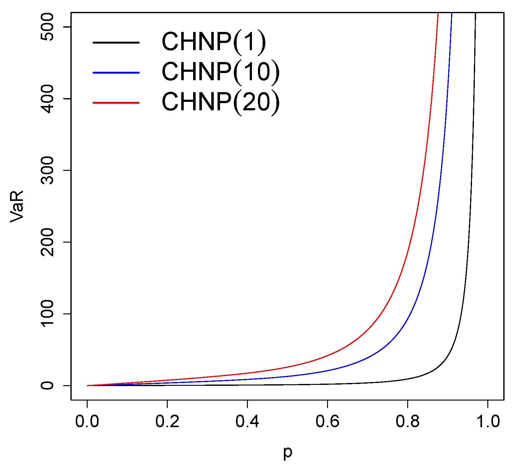
- The VaR risk measure is explicit in the CHNP model; in the applications with real data, it is compared with the VaR risk measure of the CEP and Pareto models.
- The applications with income and expenditure data show that the CHNP model provides a better fit than the CEP and Pareto models; it is also observed that the VaR of the CHNP model is closer to the empirical VaR than the VaR of the CEP and Pareto models.
- One reviewer noted the importance of performing a comparison of estimation methods, including Bayesian inference. As we have Fisher’s information for the parameter , we can use it in Jeffrey’s prior to perform Bayesian inference. However, a detailed investigation of the performance of Bayesian estimation is beyond the scope of the present paper.
Supplementary Materials
Author Contributions
Funding
Data Availability Statement
Acknowledgments
Conflicts of Interest
References
- Beirlant, J.; Teugels, J.L.; Vynckier, P. Practical Analysis of Extreme Values; Leuven University Press: Leuven, Belgium, 1996. [Google Scholar]
- Beirlant, J.; Joossens, E.; Segers, J. Generalized Pareto fit to the society of actuaries’ large claims database. N. Am. Actuar. J. 2004, 8, 108–111. [Google Scholar] [CrossRef]
- Resnick, S.I. Discussion of the Danish data on large fire insurance losses. ASTIN Bull. 1997, 27, 139–151. [Google Scholar] [CrossRef]
- Pareto, V. Cours d’Éconimie Politique; F. Rouge: Laussanne, Swizerland, 1897. [Google Scholar]
- Arnold, B.C. Pareto Distributions, 2nd ed.; Chapman & Hall: New York, NY, USA, 2015. [Google Scholar]
- Azzalini, A. A class of distributions which includes the normal ones. Scand. J. Stat. 1985, 12, 171–178. [Google Scholar]
- Henze, N. A probabilistic representation of the Skew-Normal distribution. Scand. J. Stat. 1986, 4, 271–275. [Google Scholar]
- Cooray, K.; Ananda, M.M.A. A Generalization of the Half-Normal Distribution with Applications to Lifetime Data. Commun. Stat.—Theory Methods 2008, 37, 1323–1337. [Google Scholar] [CrossRef]
- Olmos, N.M.; Varela, H.; Gómez, H.W.; Bolfarine, H. An extension of the half-normal distribution. Stat. Pap. 2012, 53, 875–886. [Google Scholar] [CrossRef]
- Olmos, N.M.; Varela, H.; Bolfarine, H.; Gómez, H.W. An extension of the generalized half-normal distribution. Stat. Pap. 2014, 55, 967–981. [Google Scholar] [CrossRef]
- Cooray, K.; Ananda, M.M.A. Modeling actuarial data with a composite lognormal-Pareto model. Scand. Actuar. J. 2005, 5, 321–334. [Google Scholar] [CrossRef]
- Scollnik, D.P.M. On composite lognormal–Pareto models. Scand. Actuar. J. 2007, 7, 20–33. [Google Scholar] [CrossRef]
- Cooray, K.; Cheng, C.I. Bayesian estimators of the lognormal–Pareto composite distribution. Scand. Actuar. J. 2015, 6, 500–515. [Google Scholar] [CrossRef]
- Ciumara, R. An actuarial model based on the composite Weibull–Pareto distribution. Math. Rep. 2006, 8, 401–414. [Google Scholar]
- Cooray, K. The Weibull–Pareto composite family with applications to the analysis of unimodal failure rate data. Commun. Stat.—Theory Methods 2009, 38, 1901–1915. [Google Scholar] [CrossRef]
- Teodorescu, S. On the truncated composite lognormal–Pareto model. Math. Rep. 2010, 12, 71–84. [Google Scholar]
- Teodorescu, S.; Panaitescu, E. On the truncated composite Weibull–Pareto model. Math. Rep. 2009, 11, 259–273. [Google Scholar]
- Teodorescu, S.; Vernic, R. Some composite exponential–Pareto models for actuarial prediction. Rom. J. Econ. Forecast. 2009, 12, 82–100. [Google Scholar]
- Scollnik, D.P.M.; Sun, C. Modeling with Weibull–Pareto models. N. Am. Actuar. J. 2012, 16, 260–272. [Google Scholar] [CrossRef]
- Calderín-Ojeda, E.; Azpitarte, F.; Gómez-Déniz, E. Modelling income data using two extensions of the exponential distribution. Physica A 2016, 461, 756–766. [Google Scholar] [CrossRef]
- Rolski, T.; Schmidli, H.; Schmidt, V.; Teugel, J. Stochastic Processes for Insurance and Finance; John Wiley & Sons: Hoboken, NJ, USA, 1999. [Google Scholar]
- Galton, F. Enquiries into Human Faculty and Its Development; Macmillan & Company: London, UK, 1883. [Google Scholar]
- Moors, J.J.A. A quantile alternative for kurtosis. J. R. Stat. Soc. Ser. D Stat. 1988, 37, 25–32. [Google Scholar] [CrossRef]
- R Core Team. R: A Language and Environment for Statistical Computing; R Foundation for Statistical Computing: Vienna, Austria, 2022; Available online: https://www.R-project.org/ (accessed on 12 January 2024).
- Artzner, P. Application of coherent risk measures to capital requirements in insurance. N. Am. Actuar. J. 1999, 3, 11–25. [Google Scholar] [CrossRef]
- Artzner, P.; Delbaen, F.; Eber, J.-M.; Heath, D. Coherent measures of risk. Math. Financ. 1999, 9, 203–228. [Google Scholar] [CrossRef]
- Klugman, S.A.; Panjer, H.H.; Willmot, G.E. Loss Models: From Data to Decisions, 4th ed.; Wiley: New York, NY, USA, 1998. [Google Scholar]
- Casella, G.; Berger, R. Statistical Inference, 2nd ed.; Cengage Learning: Boston, MA, USA, 2002. [Google Scholar]
- Akaike, H. A new look at the statistical model identification. IEEE Trans. Autom. Control 1074, 19, 716–723. [Google Scholar] [CrossRef]
- Schwarz, G. Estimating the dimension of a model. Ann. Stat. 1978, 6, 461–464. [Google Scholar] [CrossRef]
- Frees, E.W. Regression Modeling with Actuarial and Financial Applications; Cambridge University Press: Cambridge, UK, 2010. [Google Scholar]


| Increasing | Decreasing | |
|---|---|---|
| 1 | ||
| 5 |
| Model | p | VaRp | Model | p | VaRp |
|---|---|---|---|---|---|
| CHNP(0.5) | CHNP(5) | ||||
| CHNP(0.5) | CHNP(5) | ||||
| CHNP(0.5) | CHNP(5) | ||||
| CHNP(1) | CHNP(8) | ||||
| CHNP(1) | CHNP(8) | ||||
| CHNP(1) | CHNP(8) | 47,281.07 | |||
| CHNP(3) | CHNP(10) | ||||
| CHNP(3) | CHNP(10) | ||||
| CHNP(3) | CHNP(10) | 59,101.34 |
| n | Bias | SE | RMSE | CP | |
|---|---|---|---|---|---|
| 1 | 50 | 0.0420 | 0.2492 | 0.2632 | 0.9398 |
| 100 | 0.0157 | 0.1720 | 0.1758 | 0.9456 | |
| 150 | 0.0130 | 0.1402 | 0.1433 | 0.9458 | |
| 200 | 0.0130 | 0.1402 | 0.1227 | 0.9458 | |
| 2 | 50 | 0.0695 | 0.4952 | 0.5255 | 0.9391 |
| 100 | 0.0337 | 0.3443 | 0.3564 | 0.9442 | |
| 150 | 0.0216 | 0.2791 | 0.2863 | 0.9420 | |
| 200 | 0.0142 | 0.2408 | 0.2449 | 0.9454 | |
| 3 | 50 | 0.1067 | 0.7441 | 0.7928 | 0.9381 |
| 100 | 0.0631 | 0.5176 | 0.5361 | 0.9447 | |
| 150 | 0.0373 | 0.4193 | 0.4340 | 0.9411 | |
| 200 | 0.0242 | 0.3617 | 0.3700 | 0.9415 | |
| 4 | 50 | 0.0242 | 0.3617 | 1.0656 | 0.9415 |
| 100 | 0.0802 | 0.6897 | 0.7206 | 0.9413 | |
| 150 | 0.0593 | 0.5599 | 0.5703 | 0.9468 | |
| 200 | 0.0361 | 0.4829 | 0.4930 | 0.9465 |
| 0.01445457 | 0.01925126 | 0.04748003 | 0.12887746 | 0.19892610 | 0.53610582 |
| 0.70568085 | 0.72404104 | 0.78969039 | 0.82392295 | 0.84496216 | 0.90191984 |
| 0.92244296 | 1.21130369 | 1.26907096 | 1.28636763 | 1.30668599 | 1.35093138 |
| 1.42432950 | 1.65535034 | 1.72375311 | 1.84486889 | 1.96947573 | 2.10059341 |
| 2.14786935 | 2.68653223 | 2.71026918 | 2.73182813 | 3.10511668 | 3.41038988 |
| 3.57082832 | 4.44431142 | 5.09754874 | 5.21285944 | 5.60614295 | 6.62777414 |
| 8.60098244 | 9.32670082 | 10.85377372 | 14.28964739 | 20.51202824 | 25.16157611 |
| 27.74187053 | 60.16026763 | 65.41449211 | 71.33535927 | 87.67022926 | 102.51836463 |
| 183.21141945 | 215.76829133 |
| n | Median | Mean | Variance | CS | CK |
|---|---|---|---|---|---|
| 50 | 2.417 | 19.474 | 1936.553 | 0.651 | 6.477 |
| Model | ML Estimates | AIC | BIC |
|---|---|---|---|
| CHNP() | 325.641 | 329.855 | |
| Pareto() | 378.785 | 380.697 |
| n | Median | Mean | Variance | CS | CK |
|---|---|---|---|---|---|
| 500 | 21.125 | 216.709 | 11,270,001 | 0.435 | 1.655 |
| Model | ML Estimates | AIC | BIC |
|---|---|---|---|
| CHNP() | 4937.446 | 4947.875 | |
| CEP() | 5049.790 | 5054.005 | |
| Pareto() | |||
| 5867.910 | 5876.339 |
| Model∖Significance | ||||||
|---|---|---|---|---|---|---|
| CHNP() | 25.086 | 40.565 | 75.379 | 180.519 | 803.325 | 3574.872 |
| CEP() | 31.813 | 60.186 | 136.919 | 436.094 | 3159.847 | 22,895.580 |
| Pareto() | 3.744 | 13.805 | 74.248 | 795.165 | 45,800.120 | 2,638,007 |
| n | Median | Mean | Variance | CS | CK |
|---|---|---|---|---|---|
| 75 | 2.5608 | 4.9559 | 87.030 | 0.079 | 1.165 |
| Model | ML Estimates | AIC | BIC |
|---|---|---|---|
| CHNP() | 392.609 | 399.244 | |
| CEP() | 405.183 | 411.818 |
Disclaimer/Publisher’s Note: The statements, opinions and data contained in all publications are solely those of the individual author(s) and contributor(s) and not of MDPI and/or the editor(s). MDPI and/or the editor(s) disclaim responsibility for any injury to people or property resulting from any ideas, methods, instructions or products referred to in the content. |
© 2024 by the authors. Licensee MDPI, Basel, Switzerland. This article is an open access article distributed under the terms and conditions of the Creative Commons Attribution (CC BY) license (https://creativecommons.org/licenses/by/4.0/).
Share and Cite
Olmos, N.M.; Gómez-Déniz, E.; Venegas, O.; Gómez, H.W. A Composite Half-Normal-Pareto Distribution with Applications to Income and Expenditure Data. Mathematics 2024, 12, 1631. https://doi.org/10.3390/math12111631
Olmos NM, Gómez-Déniz E, Venegas O, Gómez HW. A Composite Half-Normal-Pareto Distribution with Applications to Income and Expenditure Data. Mathematics. 2024; 12(11):1631. https://doi.org/10.3390/math12111631
Chicago/Turabian StyleOlmos, Neveka M., Emilio Gómez-Déniz, Osvaldo Venegas, and Héctor W. Gómez. 2024. "A Composite Half-Normal-Pareto Distribution with Applications to Income and Expenditure Data" Mathematics 12, no. 11: 1631. https://doi.org/10.3390/math12111631
APA StyleOlmos, N. M., Gómez-Déniz, E., Venegas, O., & Gómez, H. W. (2024). A Composite Half-Normal-Pareto Distribution with Applications to Income and Expenditure Data. Mathematics, 12(11), 1631. https://doi.org/10.3390/math12111631