R-DDQN: Optimizing Algorithmic Trading Strategies Using a Reward Network in a Double DQN

Abstract

Algorithmic trading is playing an increasingly important role in the financial market, achieving more efficient trading strategies by replacing human decision-making. Among numerous trading algorithms, deep reinforcement learning is gradually replacing traditional high-frequency trading strategies and has become a mainstream research direction in the field of algorithmic trading. This paper introduces a novel approach that leverages reinforcement learning with human feedback (RLHF) within the double DQN algorithm. Traditional reward functions in algorithmic trading heavily rely on expert knowledge, posing challenges in their design and implementation. To tackle this, the reward-driven double DQN (R-DDQN) algorithm is proposed, integrating human feedback via a reward function network trained on expert demonstrations. Additionally, a classification-based training method is employed for optimizing the reward function network. The experiments, conducted on datasets including HSI, IXIC, SP500, GOOGL, MSFT, and INTC, show that the proposed method outperforms all baselines across six datasets and achieves a maximum cumulative return of 1502% within 24 months.

1. Introduction

With the rapid development of modern artificial intelligence (AI) techniques, modern machine learning is gaining more attention from scholars. In particular, the remarkable pace of development in deep learning has been evident since the introduction of various representative neural network architectures, which have led to significant achievements in the domains of CV [1,2,3], NLP [4,5,6], and time series analysis [7,8,9,10]. Using the neural network’s ability to learn latent representation, deep reinforcement learning (DRL) is receiving attention from many researchers who are trying to solve problems involving sequential decision-making. Unlike other algorithmic paradigms in machine learning that focus on prediction or classification problems, reinforcement learning algorithms learn from the outcomes of their actions, which may manifest as rewards or penalties. This unique characteristic makes reinforcement learning especially suitable for solving problems where the ideal behavior is unclear or challenging to be predefined in advance. In this case, reinforcement learning has exhibited remarkable performance in complicated domains, especially in algorithmic trading.

In the financial domain, algorithmic trading utilizes complex mathematical models and high-speed computer programs to execute trades, aiming to enhance trading efficiency and profitability while minimizing human error. With technological advancements, especially the rapid development of deep learning techniques mentioned earlier, algorithmic trading has evolved from simple automation to sophisticated systems capable of analyzing vast amounts of data, learning on their own, and making decisions. In this context, deep reinforcement learning (DRL) has received widespread attention for its potential in handling complex decision-making problems.

For deep reinforcement learning, an essential component is the reward function. Deep reinforcement learning agents receive either positive or negative reward signals from the environment for each action they take. Agents then optimize their strategy based on this reward function, aiming to maximize the accumulated reward in subsequent actions. Thus, the design of the reward function is crucial, and many studies [11] have indicated that it not only guides the actions of the agents but also influences the convergence of training. The reward function in deep reinforcement learning varies across different domains. For instance, in the Super Mario game, the design of the reward function is largely influenced by the underlying code of interactive elements within the game environment. In the algorithmic trading case, mainstream reward functions, such as the Sharpe ratio, are designed based on guiding theories in the financial field. These theories often give the trading strategies of the agents a certain preference, such as a preference for risk avoidance or a desire to increase returns. Works related to deep reinforcement learning based on these reward function designs have made significant breakthroughs in recent years. The design of reward functions in the financial domain heavily relies on the expertise of financial professionals. This is because the designers of reward functions need to consider factors including but not limited to investment objectives, risk preferences, asset classes, transaction costs, market liquidity, financial indicators, and more. These factors often require specialized knowledge in the financial domain for understanding and balancing. However, different experts often have different investment preferences. Avoiding such discrepancies and selecting more generalized reward functions will become new challenges for researchers. In this case, a method that does not have to rely heavily on human expert investment preferences and specialized knowledge is required. More importantly, it should be able to incorporate expert knowledge into algorithms.

Therefore, employing neural networks to learn a reward function model with a certain level of interpretability and usability has become a viable solution. Moreover, the idea of RLHF, a method capable of incorporating expert experience data into reinforcement learning algorithms, has emerged as a potential approach for the aforementioned solution. Reinforcement learning with human feedback (RLHF) is an approach that seeks to refine the architecture of deep reinforcement learning by integrating human expertise directly into the training process. Recently, numerous large language models [12,13] have started incorporating demonstrations, feedback, and explanations from human experts during their training phases. This inclusion of human insight not only bridges the gap between theoretical model performance and practical application effectiveness but also significantly boosts the models’ capabilities.

Inspired by these advancements, this paper introduces the reward-driven double DQN algorithm. This innovative algorithm pioneers the introduction of a reward network into the deep reinforcement learning architecture, which dynamically generates reward signals based on the current state and the actions taken by the agent. This network is trained through supervised learning using pre-generated pairs of expert actions and rewards. In this study, a hypothesis was proposed that with the help of the reward function network, the performance of the traditional deep reinforcement learning algorithm DDQN will be improved in the financial trading environment. Also, the proposed R-DDQN should have significant trading performance that outperforms baselines across all datasets.

The main contributions of this paper are listed as follows:

• Exploring the use of RLHF in single-asset trading, which utilizes the TimesNet reward network to dynamically generate reward signals.
• Combining the concept of RLHF and algorithmic trading enables agents to utilize reward signals from human experts, which improves the overall performance of reinforcement learning algorithms.
• Using a training method that is commonly used in classification tasks to train reward networks. The experimental results show that the reward network trained by this method not only ensures the convergence of deep reinforcement learning algorithms but also improves trading performance.
• Assessments across six commonly-used datasets covering HSI, IXIC, SP500, GOOGL, MSFT, and INTC, reveal that the proposed algorithm markedly surpasses numerous traditional and deep reinforcement learning (DRL)-based approaches. These findings underscore the algorithm’s capacity to bolster stock trading strategies and its ability to greatly improve the consistency of algorithmic trading by integrating Reinforcement Learning with human feedback.

This paper is structured as follows. In Section 2, previous studies on the topic are discussed. Section 3 explains the proposed method in detail. The experimental results are described and analyzed in Section 4. The discussion of this research is described in Section 5. Finally, Section 6 summarizes the results and shows future works.

2. Related Works

To enhance the understanding of the similarities and differences within the scope of the literature addressed by the proposed method, two distinct strands of research have been examined: reinforcement learning with human feedback and algorithmic trading. Discussing and introducing the related studies allows a concentrated and structured exploration of current research.

2.1. Reinforcement Learning with Human Feedback

Reinforcement learning with human feedback (RLHF) is an approach that enhances traditional reinforcement learning (RL) by integrating human feedback into the learning process. This method is particularly useful in scenarios where it might be challenging to define an appropriate reward function or when the environment is too complex for standard RL algorithms to navigate successfully without guidance. To address this problem, RLHF leverages the efficiency of machine learning algorithms to process and learn from large amounts of data, while also incorporating the nuanced understanding and ethical considerations that humans can provide. This combination allows the system to learn behaviors that are not only effective in achieving a task but also align with human values and expectations [14,15].

In recent years, research based on RLHF (reinforcement learning with human feedback) has led to groundbreaking advancements in various fields. For instance, the remarkable progress achieved in the field of artificial intelligence, particularly with large language models [13,16,17], owes much to expert demonstrations or feedback used to assist model training. This approach enables models to cope with complex and dynamic environments. Furthermore, large language models based on the RLHF principle have also made remarkable achievements in the financial domain. Kelvin et al. [18] developed a large model, building upon GPT [5] and Vicuna [19], which is capable of predicting stock price trends and providing corresponding explanations for these trends. The training of this model requires a dataset containing expert explanations of stock price trends, along with the self-reflective approach proposed in their paper. Experimental results demonstrate that this model can accurately predict changes in stock prices and generate appropriate explanations. Their work not only illustrates the potential of large language models to be applied extensively in the financial domain but also underscores the potential of RLHF-based approaches for research in financial trading.

2.2. Algorithmic Trading

Algorithmic trading is a trading strategy that involves the use of computer programs to execute high-speed, high-volume trades. This trading strategy relies on predefined rules and parameters, automatically executing trade orders by analyzing and simulating market data. Algorithmic trading is characterized by its rapid response to market changes and its ability to capitalize on short-term price fluctuations, often completing trade decisions and executions within milliseconds [20].

The rise in the popularity of algorithmic trading can be attributed to advancements in technology, the availability of vast amounts of data, and the expansion of high-frequency trading. In financial markets such as equities, futures, and foreign exchange, where swift and precise trade executions are crucial, algorithmic trading has become widespread. These methods have notably improved market liquidity, as evidenced by their impact on various trading platforms [21,22,23]. The incorporation of machine learning algorithms into financial trading has garnered significant attention recently, offering a potent means to automate and refine trading processes. These algorithms provide traders with a more adaptable, data-driven, and impartial approach to navigating financial markets. Through the utilization of machine learning, traders can optimize their returns on investment while effectively managing risk, signaling a shift toward a more sophisticated and analytical trading approach.

Algorithmic trading encompasses a wide range of research directions, including cryptocurrency trading [24,25,26,27], single asset stock trading [28,29,30,31,32], risk management [33,34], post-trade analysis [35], and more, all with the aim of enhancing the efficiency, profitability, and resilience of trading strategies. Experimental results from these studies suggest that algorithmic trading methods integrated with advanced machine learning technologies offer advantages such as adaptability to changing market conditions, avoidance of emotional bias, and acceleration of trading speed—benefits that were challenging to achieve with previous conventional methods. Hence, with the rapid evolution of AI technology today, the algorithmic trading field holds substantial research potential.

3. Methods

In algorithmic trading, the process by which trading entities select and execute trading strategies can be regarded as a Markov decision process, and for this reason, algorithmic trading can be viewed as a reinforcement learning problem. Under this premise, financial reinforcement learning agents need to learn the optimal trading strategy by exploring the feedback from different actions in the trading environment. However, since this article aims to explore the application of reinforcement learning in complex financial environments, to ensure the reliability of the conclusions, the following assumptions are required:

• The market operates with full efficiency. This implies that all existing information is perfectly reflected in market prices, without being influenced by any external factors that might affect the market.
• Considering the complexities surrounding stock market liquidity and the relatively modest scale of assets under scrutiny, particularly from the perspective of individual investors, this paper posits that the influence of singular buy or sell orders on market prices is minimal.
• No slippage in the execution of orders, suggesting that the liquidity of the market assets is adequate for executing trades at the established prices.

3.1. Overview of the Proposed Method

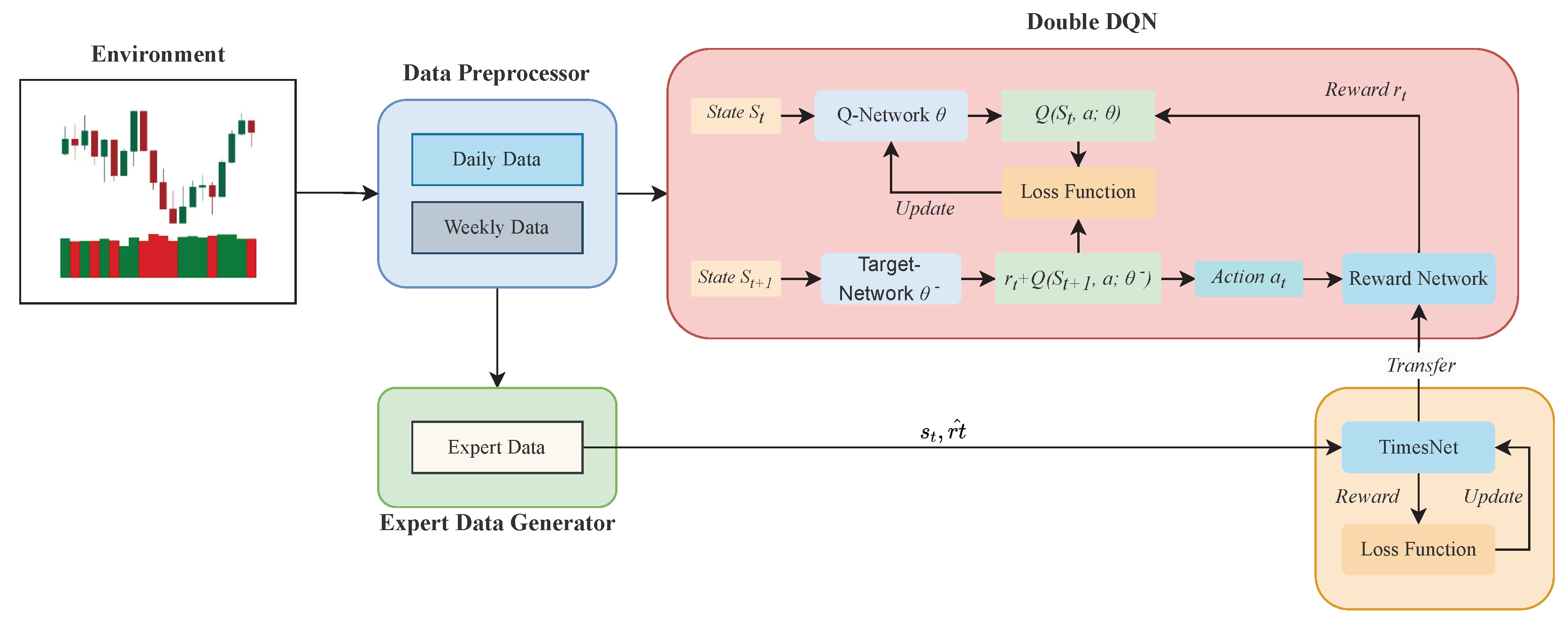
In this section, a brief overview of the proposed method is presented. As illustrated in Figure 1, a new algorithmic framework is created by integrating the reward function network obtained through supervised training with traditional deep reinforcement learning methods. This framework can be divided into two main parts. First, the training data is obtained from an observable environment. In Figure 1, the environment is represented by a simple candlestick chart, where red bars indicate a price decrease, while green bars indicate a price increase. Then, data are processed into daily and weekly datasets. The daily data capture the subtle fluctuations in stock prices from day to day, while the weekly data describe the overall weekly changes in the stock market. By preprocessing the data in this manner, the agent cannot only focus on potential gains from minor price movements but also avoid risks based on changes in overall trends. Second, a reward function network is introduced, replacing the predefined reward function in deep reinforcement learning. This reward network takes the current state as input and outputs the reward value for each possible trading action. To train this network, expert labels generated based on certain rules are introduced into the network’s supervised training as training data. Subsequently, the pre-trained reward function network is integrated into the double DQN (DDQN) method, facilitating the learning of effective trading strategies.

3.2. Problem Formulation

3.2.1. State

The state represents a description of the environment at time t, providing the agent with the information it needs to make decisions. As mentioned earlier, data used in training are processed as daily data and weekly data. In this case, the state can be treated as a daily state or a weekly state. Denoted as $s_t^d$, the daily state represents the collection of the opening price, high price, low price, closing price, and trading volume for the previous n days. The daily state can be denoted as follows:

$$s_t^d={\{O_n^d,H_n^d,L_n^d,C_n^d,V_n^d\}}_t,$$

(1)

where $O_n^d,H_n^d,L_n^d,C_n^d,V_n^d$ are the stock market prices for the opening, highest, lowest, closing, and total trading volume in the past n days. Similarly, the weekly state can be represented as follows:

$$s_t^w={\{O_n^w,H_n^w,L_n^w,C_n^w,V_n^w\}}_t,$$

(2)

where $O_n^w,H_n^w,L_n^w,C_n^w,V_n^w$ are the stock market prices for the opening, highest, lowest, closing, and total trading volume in the weekly period of the past n days. The complete state at time t is the concatenation of daily state and weekly state, therefore, state $s_t$ can be denoted as follows:

$$s_t=\{s_t^d,s_t^w\},$$

(3)

3.2.2. Action

At each time step, t, given a state, $s_t$, the agent selects and performs an action, $a_t$, guided by the RL policy. In this study, which focuses on algorithmic trading, the agent has only three actions, namely buy, hold, and sell. The computation of actions can be represented as follows:

$$a_t=\left\{\begin{array}{cc}-1,\hfill & \mathrm{if}\pi \left(a_t\right|s_t)=\mathrm{Sell};\hfill \\ 0,\hfill & \mathrm{if}\pi \left(a_t\right|s_t)=\mathrm{Hold};\hfill \\ 1,\hfill & \mathrm{if}\pi \left(a_t\right|s_t)=\mathrm{Buy},\hfill \end{array}\right.$$

(4)

where $\pi \left(a_t\right|s_t)$ is the RL policy that is computed by the policy network of reinforcement learning agent at time step t.

However, the actual trading operation executed by the agent is not necessarily the same as the trading signal generated by the policy network. For example, if the accounts already holding a long position (${\mathrm{POS}}_t=1$), a buy signal indicates maintaining a long position. In this case, the actual action is held instead of buying. This is because the trading rules do not allow for additional buying while in a long position, and similarly, do not allow for further short selling while in a short position.

Table 1. Actual trading operations based on the signal and the current account position.

Position (${\mathbf{POS}}_{\mathit{t}}$)	Signal (${\mathit{a}}_{\mathit{t}}^{\ast }$)	Actual Action (${\mathit{a}}_{\mathit{t}}$)	Description
0	0	0	Hold the cash.
0	1	1	Open a long position.
0	$-1$	$-1$	Open a short position.
1	0	0	Hold the long position.
1	1	0	Hold the long position.
1	$-1$	$-1$	Close the long position.
$-1$	0	0	Hold the short position.
$-1$	1	1	Close the short position.
$-1$	$-1$	0	Hold the short position.

explains the details of the actual trading operations determined by a combination of the current account positions and trading signals.

3.3. Reward Function Network

3.3.1. Expert Demonstration Data

The reward function is an essential component of deep reinforcement learning, where each action taken by the agent causes changes in the environment, and the environment, in turn, provides feedback to the agent. This feedback can be either positive or negative, determined by the specific reward function. As discussed in the previous text, due to the complexity of the financial markets, it is challenging for a single reward function to achieve similar returns across multiple stocks or indices. Therefore, learning the underlying reward and punishment mechanisms from human expert trading behaviors becomes a way to address the above issue. In this study, a reward function network based on TimesNet is employed to replace the predefined reward function in reinforcement learning. For the network’s training, a set of rules for generating expert demonstration data is introduced, providing training data for the reward function network’s supervised training.

A set of expert demonstration data generation rules is adopted to calculate reward values based on stock price movements and trading actions. It evaluates the highest returns across various positions with an adjustable time window, allowing for the efficient capture of market trends to maximize returns. The function’s adaptability enables customization towards short-term or long-term trends by adjusting the time horizon parameter, m, suited to the specific characteristics of the stocks. The mathematical expression of this rule is detailed in Equations (5)–(7):

$$R_t=\left\{\begin{array}{cc}{\mathrm{POS}}_t\ast \mathrm{maxRatio},\hfill & \begin{array}{c}\mathrm{maxRatio}>0\mathrm{or}\hfill \\ \mathrm{maxRatio}+\mathrm{minRatio}>0,\hfill \end{array}\hfill \\ \mathrm{const}-(\mathrm{maxRatio}-\mathrm{minRatio}),\hfill & {POS}_t=0,\hfill \\ {\mathrm{POS}}_t\ast \mathrm{minRatio},\hfill & \begin{array}{c}\mathrm{minRatio}<0\mathrm{or}\hfill \\ \mathrm{maxRatio}+\mathrm{minRatio}<0,\hfill \end{array}\hfill \end{array}\right.$$

(5)

where const is a scalar and ${POS}_t$ denotes a trading position at time t. In this study, trading positions include long (${POS}_t$ = 1), short (${POS}_t$ = $-1$) and hold (${POS}_t$ = 0).

The maxRatio and minRatio shown in Equation (5) illustrate the max price change and min price changes in the following m days, which can be denoted as follows:

$$\mathrm{maxRatio}=\left\{\begin{array}{cc}\max (r_{t+1},r_{t+2},\cdots ,r_{t+m}),\hfill & \mathrm{if}{r}_{t+i}>0,\hfill \\ 0,\hfill & \mathrm{otherwise}.\hfill \end{array}\right.$$

(6)

$$\mathrm{minRatio}=\left\{\begin{array}{cc}\min (r_{t+1},r_{t+2},\cdots ,r_{t+m}),\hfill & \mathrm{if}{r}_{t+i}<0,\hfill \\ 0,\hfill & \mathrm{otherwise},\hfill \end{array}\right.$$

(7)

where $r_{t+i}=\frac{p_{t+i}-p_t}{p_t}\ast 100$.

In the design of this research, the reward function network generates reward values for all possible trading actions after observing state $s_t$. In this study, actions that an agent or an expert can execute include buying, selling, and holding. Therefore, the expert reward label for state $s_t$ can be represented as follows:

$$r_t=[r_t^{\mathrm{hold}},r_t^{\mathrm{buy}},r_t^{\mathrm{sell}}].$$

(8)

3.3.2. Loss Function of Reward Function Network

As described earlier, the actions of the agent can be divided into [buy, hold, sell], correspondingly, the reward labels in the expert demonstration data can also be divided into $[r_t^{\mathrm{hold}},r_t^{\mathrm{buy}},r_t^{\mathrm{sell}}]$. Based on this characteristic, the loss function used in the training phase of the reward function network has been redesigned. Specifically, a training method similar to a classification task for training the reward function network is adopted. First, the softmax function is used to convert the reward labels of the expert demonstration data and the predictions outputted by the reward function network into probability values, expressed as follows:

$$r_t^{\sigma }=\mathrm{softmax}\left(r_t\right)$$

(9)

$${\widehat{r}}_t^{\sigma }=\mathrm{softmax}\left({\widehat{r}}_t\right)$$

(10)

where $r_t$ is the expert reward label and ${\widehat{r}}_t$ is the reward label output by the reward function network.

Then, cross-entropy is used to calculate the loss function between $r_t^{\sigma }$ and ${\widehat{r}}_t^{\sigma }$, expressed as follows:

$$H(r_t^{\sigma },{\widehat{r}}_t^{\sigma })=-\sum _i({\left[r_t^{\sigma }\right]}_{i}log\left({\left[{\widehat{r}}_t^{\sigma }\right]}_i\right)),$$

(11)

where i represent the $i_{th}$ elements in the reward label. Figure 2 illustrates this training logic.

3.4. Reward-Driven Double DQN

In this paper, reward-driven double DQN (R-DDQN) is proposed to explore trading strategy in a financial environment based on double DQN [36]. The double deep Q network (DDQN) is a method to address the overestimation problem in Q-learning algorithms [37] within reinforcement learning. In a traditional DQN (deep Q network), the same network is used for both selecting and evaluating actions, which can lead to overestimation of Q-values. DDQN addresses this issue by introducing two structurally identical but parametrically distinct neural networks: a primary network $\theta$ for selecting the best action and a target network ${\theta }^{-}$ for evaluating the value of that action.

At every timestep t, the agent takes an action $a_t$, formalizing a transition $(s_t,a_t,r_t,s_{t+1})$, where $s_t$ is the current state, $r_t$ is the reward computed by the task-specific reward function, and $s_{t+1}$ is the next state. With the transition, the primary network $\theta$ selects the next action $a_{t+1}^{\max }$

$$a_{t+1}^{\max }(s_{t+1};\theta )={\mathrm{argmax}}_{a_{t+1}}Q(s_{t+1},a_{t+1};\theta ).$$

(12)

Target network ${\theta }^{-}$, on the other hand, estimates the Q value with the formula $Q(s_{t+1},a_{t+1}^{\max };{\theta }^{-})$. With the estimation from the target network, the double DQN algorithm can calculate the temporal difference target. This target signifies an estimation of the expected cumulative reward that the agent employs to refine its value function during the update:

$$y=r_t+\gamma Q(s_{t+1},a_{t+1}^{\max }(s_{t+1};\theta );{\theta }^{-}),$$

(13)

where $\gamma$ is a discounted factor. Finally, the primary network performs gradient descent with loss, as follows:

$$L\left(\theta \right)=r_t+\gamma Q(s_{t+1},a_{t+1}^{\max }(s_{t+1};\theta );{\theta }^{-})-Q(s_t,a_t;\theta ).$$

(14)

Here, instead of computing the reward by using the task-specific reward function, $r_t$ is predicted by the pre-trained reward function network $\omega$. $\omega$ takes state, $s_t$, and action, $a_t$, as input, and then outputs the corresponding reward at timestep t. The mathematical equation can be denoted as follows:

$$r_t=\omega (s_t,a_t).$$

(15)

Therefore, the loss of the primary network in the reward-driven DDQN can be represented as follows:

$$L\left(\theta \right)=\omega (s_t,a_t)+\gamma Q(s_{t+1},a_{t+1}^{\max }(s_{t+1};\theta );{\theta }^{-})-Q(s_t,a_t;\theta ).$$

(16)

3.5. R-DDQN Training

The training procedure of R-DDQN is illustrated in Algorithm 1. Initially, an expert demonstration dataset consisting of state–reward pairs is used to train a reward function network. This dataset is generated through pre-designed rules. The reward values $\widehat{r_t}$ predicted by the reward function network, and $r_t$ in the expert demonstration dataset, are subjected to a softmax function, turning these reward values into probabilities between 0 and 1. Subsequently, the error between the predicted and actual values is calculated using the cross-entropy loss function. The parameters of the reward function network $\omega$ are updated through the gradient descent of this error. Once the training of $\omega$ is finished, the reward function network is transferred to the DDQN algorithm, where it is used in place of the DDQN’s reward function. Afterward, a series of data from financial markets is introduced and forms the base environment for the reinforcement learning algorithm. The agent executes trading actions, and these actions, along with the current state, are input into the reward function network, which then generates reward values. These reward values are fed back to the agent, which updates its own network based on these rewards and then executes the next action. This training of the DDQN agent continues until the agent’s trading strategy tends toward stability.

Algorithm 1: R-DDQN algorithm

Input: $\mathcal{B}$—empty replay buffer; $\theta$—initial network parameters, ${\theta }^{-}$—copy of $\theta$; $N_r$—replay buffer maximum size; $N_b$—training batch size; $N^{-}$—target network replacement frequency, ${\omega }_p$—reward function network parameter, $\alpha$—learning rate.

4. Experiment

4.1. Dataset

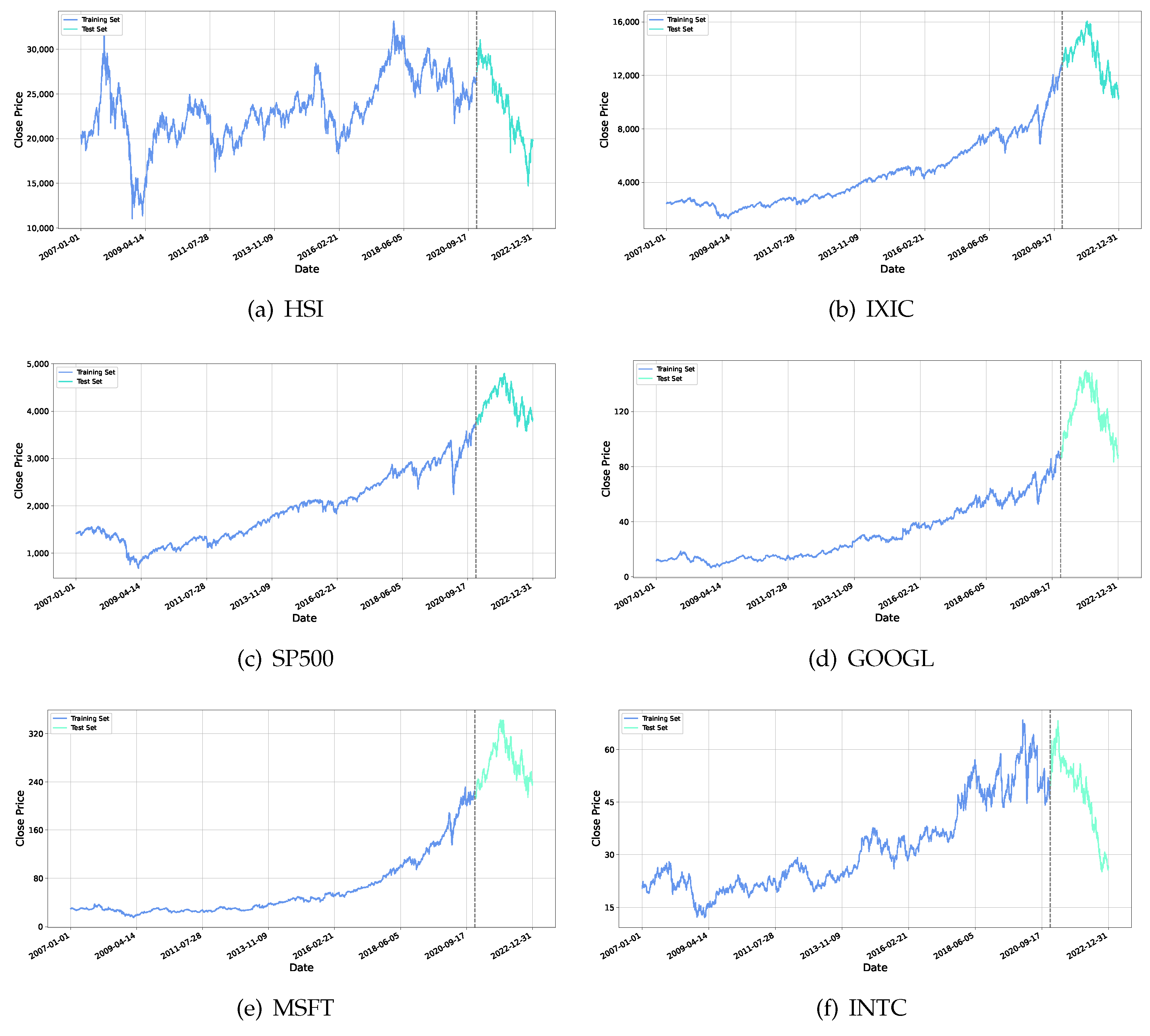
This research incorporates data from three major stock indices: the Hang Seng Index (HSI) of Hong Kong, the United States NASDAQ Composite (IXIC), and S&P 500 (SP500), in addition to three individual stocks: Google (GOOGL), Microsoft (MSFT), and Intel (INTC). The data span from 1 January 2007 to 31 December 2022, providing an extensive dataset for model training.

The data are organized into two subsets for model training and evaluation. Each subset contains five-dimensional time series data for each stock and index, detailing daily opening prices, lowest prices, highest prices, closing prices, and trade volumes. Figure 3 presents the closing prices for each index. The training dataset, which covers the period from 1 January 2007 to 31 December 2020, is used to tune the model parameters. The testing dataset, spanning from 1 January 2021 to 31 December 2022, serves to test the models’ performance. In all close price curves, the blue part represents the training set and the orange part represents the test set. Additionally, to ensure the stability of the datasets, the original data, including both the training and testing sets, are normalized. The normalization process is conducted as follows:

$${\widehat{x}}_t=\frac{x_t-\mu }{\sigma },$$

(17)

where $x_t$ represents the original price at time t, while $\mu$ and $\sigma$ represent the sample mean and sample standard deviations of the dataset, respectively.

4.2. Baseline Methods and Evaluation Metrics

To objectively evaluate the performance of the proposed method, several DRL algorithms and traditional financial trading methods are introduced as baselines for this study. These baselines include TDQN, MLP-Vanilla, DQN-Vanilla, B&H, S&H, MR, and TF. The proposed method will be compared with the aforementioned baselines in several evaluation metrics, including the CR (cumulative return), AR (annualized return), SR (Sharpe ratio), and MDD (maximum drawdown). For all baselines and the proposed method in this research, a 0.3% cost for each transaction has been used.

4.3. Experiment Setup

The method proposed in this research is trained across six distinct datasets. The performance of the model is evaluated by a test set associated with its respective dataset. The finely tuned hyperparameters for the agent in this experiment are detailed in

Table 2. The tuned hyperparameters.

Hyperparameter	R-DDQN
Number of CNN layers	13
Number of linear layers	2
Activation function	GELU
Learning rate ($\alpha$)	0.001
Replay memory size	1000
Discount factor	0.9
Window size	20

. The computational resources utilized in this study are specified as follows: The central processing unit (CPU) employed was the 13th Generation Intel(R) Core(TM) i7-13700KF. Graphics processing was managed by an NVIDIA RTX 4090 GPU, boasting 24 GB of memory. On the software front, the study employed Python version 3.10, PyTorch version 1.12, and CUDA version 12.1. The operating system was Windows 10.

4.4. Analysis of Pre-Trained Reward Network and Policy Network

As discussed earlier, the method proposed in this paper involves integrating a pre-trained reward function network with the double DQN (DDQN) algorithm, allowing this network to replace the reward function in the DDQN algorithm. Consequently, selecting an appropriate model for the reward network will significantly impact the results of this study. In this context, three neural network architectures, TimesNet [38], PatchTST [8], and DLinear [39], which have shown remarkable performance in the time series domain, have been introduced into the experiment. To assess the compatibility of the three network structures with this study, each network has been trained on six datasets with daily and weekly data mentioned earlier, comparing their classification accuracy on both training and testing sets.

Table 3. The classification accuracy of the reward function network on six datasets.

Indexes	Dataset	TimesNet	PatchTST	DLinear
HSI	Training	85.44%	69.6%	70.48%
	Test	69.38%	71.52%	72.38%
IXIC	Training	92.91%	67.66%	68.20%
	Test	67.36%	71.13%	71.97%
S&P500	Training	92.69%	67.46%	66.77%
	Test	64.23%	66.53%	67.99%
GOOGL	Training	92.57%	71.74%	72.17%
	Test	71.55%	73.01%	72.80%
MSFT	Training	87.54%	70.43%	70.74%
	Test	71.55%	70.92%	70.71%
INTC	Training	88.46%	72.34%	68.57%
	Test	70.71%	71.34%	71.97%
Average	Training	89.94%	69.87%	69.49%
	Test	69.13%	70.74%	71.30%

The bolded parts represent the best experimental results.

depicts the experimental results for three networks.

From Table 3, it is evident that the three networks produced closely competitive results across the six datasets, with most of the classification accuracies around 70%, and the lowest accuracy being 64.23%, as observed for TimesNet in the S&P 500 dataset. The largest discrepancy among the networks was seen in the IXIC dataset test results, where DLinear outperformed TimesNet by an accuracy of 4.31%. This indicates that the performances of the three networks in the test datasets were quite comparable, with DLinear showing the best overall performance. However, a significant gap is noticeable when observing their performance in the training datasets. TimesNet was the best performer among the three on the training set, with all accuracies above 85%, and the lowest performance at 85.44%. In contrast, the PatchTST and DLinear performances in the training sets were less impressive, with most accuracies hovering around 70%; there were several instances where the training set accuracies were lower than those in the test sets, suggesting a risk of underfitting for these two networks. Although DLinear performed better in the test sets, it is crucial to note that the reward function network plays a role in deep reinforcement learning algorithms only during the training phase. In this phase, the agent takes action, and the reward function network provides feedback based on the action and current state to the agent, which then updates its network based on the reward. During the testing phase, the agent selects an action based on the current state without learning from the reward function network’s output. Therefore, based on the experimental results and theoretical considerations, TimesNet will be chosen as the model for the reward function network.

It is also necessary to decide the network structure for the agent’s policy network. Given that the method proposed in this paper is based on double deep Q networks (DDQNs), the three networks previously mentioned will each be tested as the Q network of DDQN on the HSI dataset. The DDQN’s reward function will be Equation (5). From

Table 4. The performance of DDQN with three networks in HSI.

Metrics	DDQN-TimesNet	DDQN-PatchTST	DDQN-DLinear
CR	576.54%	391.70%	417.00%
AR	141.71%	121.26%	124.60%
SR	4.51	3.815	3.978
MDD	9.29%	8.76%	4.04%

, it can be observed that the DDQN based on TimesNet significantly outperforms the others in all four metrics. Its cumulative return is nearly 200% higher than the others, and it boasts the highest Sharpe ratio and annualized return. Although its maximum drawdown (MDD) is not the lowest, its overall performance across the four metrics remains the best. This is the reason why TimesNet is selected as the agent’s network.

4.5. Comparison with Baselines

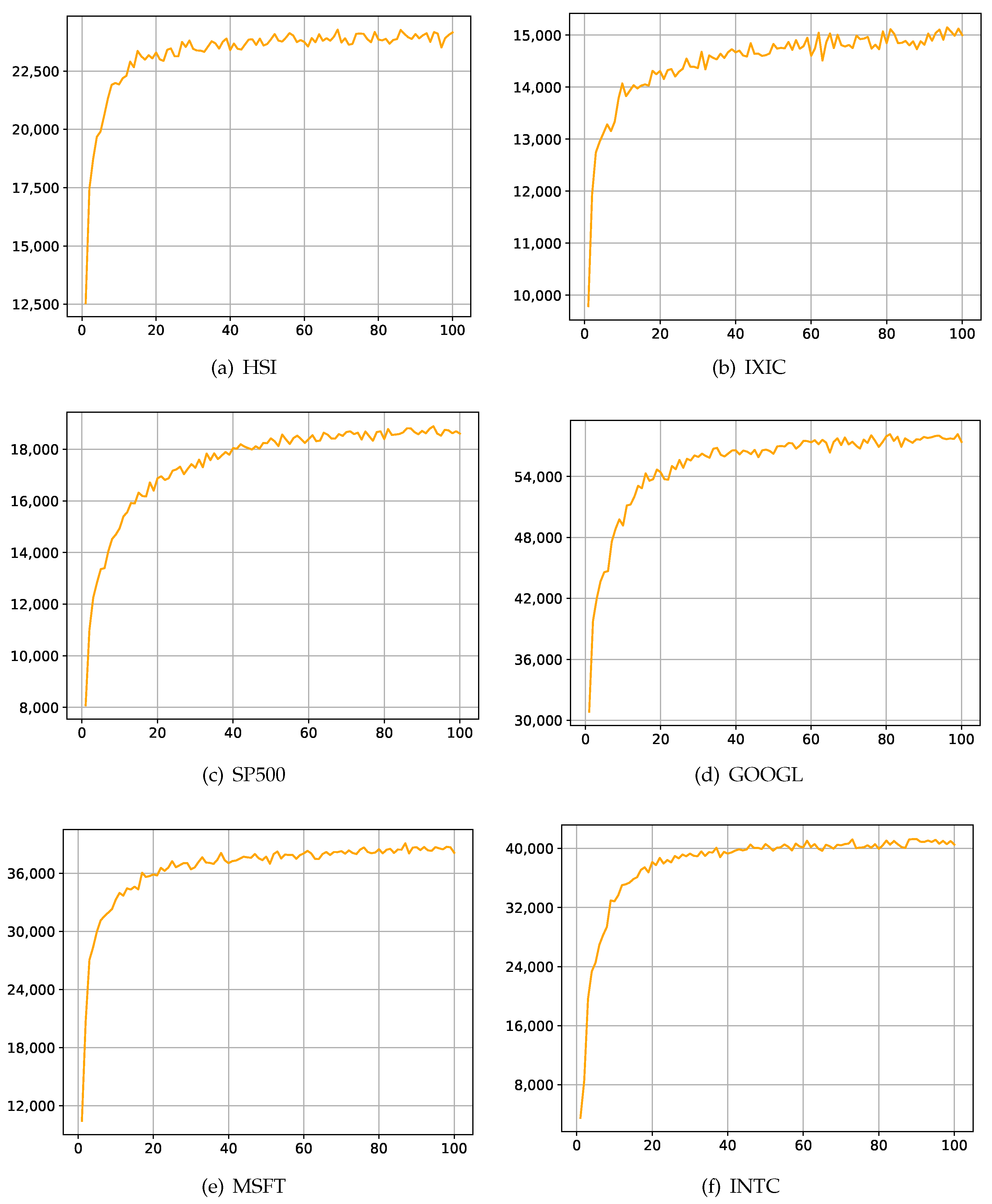
To assess the effectiveness of the method proposed in this paper, performance evaluation is conducted from two perspectives. First, convergence is crucial for machine learning algorithms, as it is an important indicator of model reproducibility and robustness. In this article, the accumulated reward, which is the total sum of rewards obtained by an agent along a complete trajectory, is used to measure whether the agent’s training converges. If the accumulated reward remains stable over consecutive epochs without sudden significant increases or decreases, it indicates that the agent’s training has converged. Figure 4 illustrates the training of the proposed algorithm on six datasets. Here, the horizontal axis represents epochs, while the vertical axis represents accumulated reward. It can be observed that in the training of all six datasets, the accumulated reward tends to stabilize after approximately 20 epochs, and there are no significant increases or decreases in the subsequent dozens of epochs. Therefore, it can be concluded that the algorithm proposed in this paper demonstrates excellent convergence.

Secondly, the method proposed in this paper needs to be compared with several baselines mentioned earlier in the test sets of the six datasets, using four metrics to measure their strengths and weaknesses in various aspects. Additionally, since R-DDQN is based on the DDQN algorithm, the classical DDQN algorithm will also serve as one of the baselines. Here, both the DDQN algorithm and R-DDQN employ the same selection of the agent network, with the only difference being that DDQN directly uses Equation (5) as the reward function, while R-DDQN replaces it with a reward network.

Table 5. The performance of various trading approaches on six datasets.

Datasets	Metrics	B&H	S&H	MR	TF	TDQN	DQN-Vanilla	MLP-Vanilla	DDQN	R-DDQN
HSI	CR ↑	−5.51%	5.51%	−3.10%	−2.80%	−44.71%	18.62%	−9.92%	576.54%	601.06%
	AR↑	−23.34%	21.23%	−9.50%	−8.94%	−31.76%	16.18%	−6.98%	141.71%	145.05%
	SR↑	−0.68	0.92	−0.26	−0.273	−1.09	0.51	−0.39	4.51	4.81
	MDD↓	45.38%	11.11%	30.22%	32.69%	59.49%	22.34%	22.57%	9.29%	8.95%
IXIC	CR↑	−3.77%	3.77%	−1.56%	−3.91%	−22.95%	32.03%	−20.85%	709.00%	790.00%
	AR↑	−12.38%	17.34%	−2.18%	−14.11%	−10.51%	23.45%	−12.83%	148.83%	154.76%
	SR↑	−0.33	0.51	−0.06	−0.43	−0.40	0.75	−0.33	5.21	5.55
	MDD↓	33.86%	22.87%	31.17%	26.42%	35.87%	26.61%	35.72%	3.89%	4.35%
SP500	CR↑	0.05%	−0.05%	1.46%	−1.57%	0.04%	54.38%	−3.35%	331.03%	459.83%
	AR↑	4.89%	1.90%	7.91%	−4.06%	1.84%	32.56%	−0.85%	106.84%	123.88%
	SR↑	0.16	0.05	0.30	−0.15	0.10	1.49	−0.03	4.72	5.81
	MDD↓	25.05%	26.70%	16.06%	24.28%	25.38%	13.54%	18.63%	5.51%	2.36%
GOOGL	CR↑	−1.07%	1.07%	1.13%	−6.97%	−11.08%	185.13%	1.92%	1424.87%	1502.26%
	AR↑	3.41%	30.05%	11.76%	−28.25%	−1%	71.52%	8.78%	189.88%	192.58%
	SR↑	0.07	0.34	0.25	−0.59	−0.03	2.28	0.19	5.40	5.70
	MDD↓	44.31%	58.29%	25.37%	47.21%	44.12%	17.03%	44.32%	4.82%	4.82%
MSFT	CR↑	0.76%	−0.76%	10.52%	−2.42%	−15.74%	150.56%	121.45%	563.27%	944.29%
	AR↑	9.23%	9.37%	38.02%	−4.58%	−4.65%	63.68%	56.26%	136.90%	165.35%
	SR↑	0.21	0.15	0.93	−0.11	−0.16	2.06	1.79	4.22	5.42
	MDD↓	37.11%	47.04%	33.56%	39.76%	50.93%	15.29%	19.63%	6.56%	6.52%
INTC	CR↑	−9.90%	9.90%	4.46%	−4.72%	−55.33%	82.04%	34.87%	984.45%	1136.69%
	AR↑	−49.35%	35.91%	23.49%	−14.33%	−45.1%	44.38%	25.48%	169.45%	177.61%
	SR↑	−0.90	0.92	0.49	−0.30	−1.06	1.32	0.72	4.44	4.67
	MDD↓	61.60%	21.14%	31.57%	54.17%	63.96%	12.28%	27.53%	8.42%	6.36%

The bolded parts represent the best experimental results.

describes the comparison between R-DDQN and other baselines.

From Table 5, it is evident that the method proposed in this paper—R-DDQN—achieves the highest cumulative return (CR) across all six datasets. The highest CR reaches 1502.26%, while the lowest is 459.83%. Among the baselines, only DDQN with TimesNet achieves CR close to R-DDQN, while other baselines rarely exceed 100% CR. Observing other metrics, across all datasets, R-DDQN not only achieves the highest CR but also attains the highest average return (AR) and Sharpe ratio (SR). Regarding the maximum drawdown (MDD), R-DDQN is only outperformed by DDQN on the IXIC dataset, with the difference between the two not exceeding 0.5%. Therefore, based on the observation of these metrics, it can be concluded that R-DDQN effectively captures and understands the stock price patterns and trends inherent in the training data, thereby outputting excellent trading strategies.

4.6. Analysis of Trading Strategy

After the performance of the R-DDQN agent on the six datasets has been analyzed using multiple metrics, further evaluation is necessary.

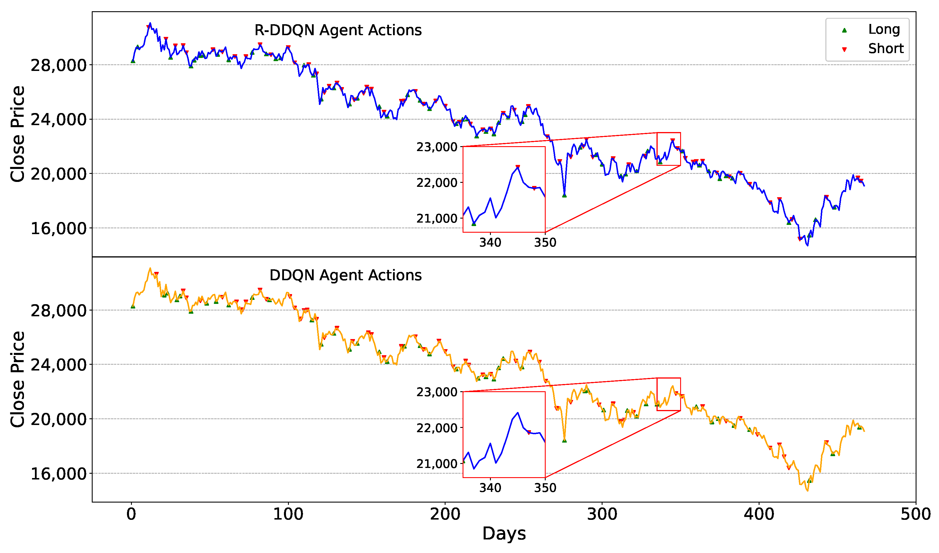
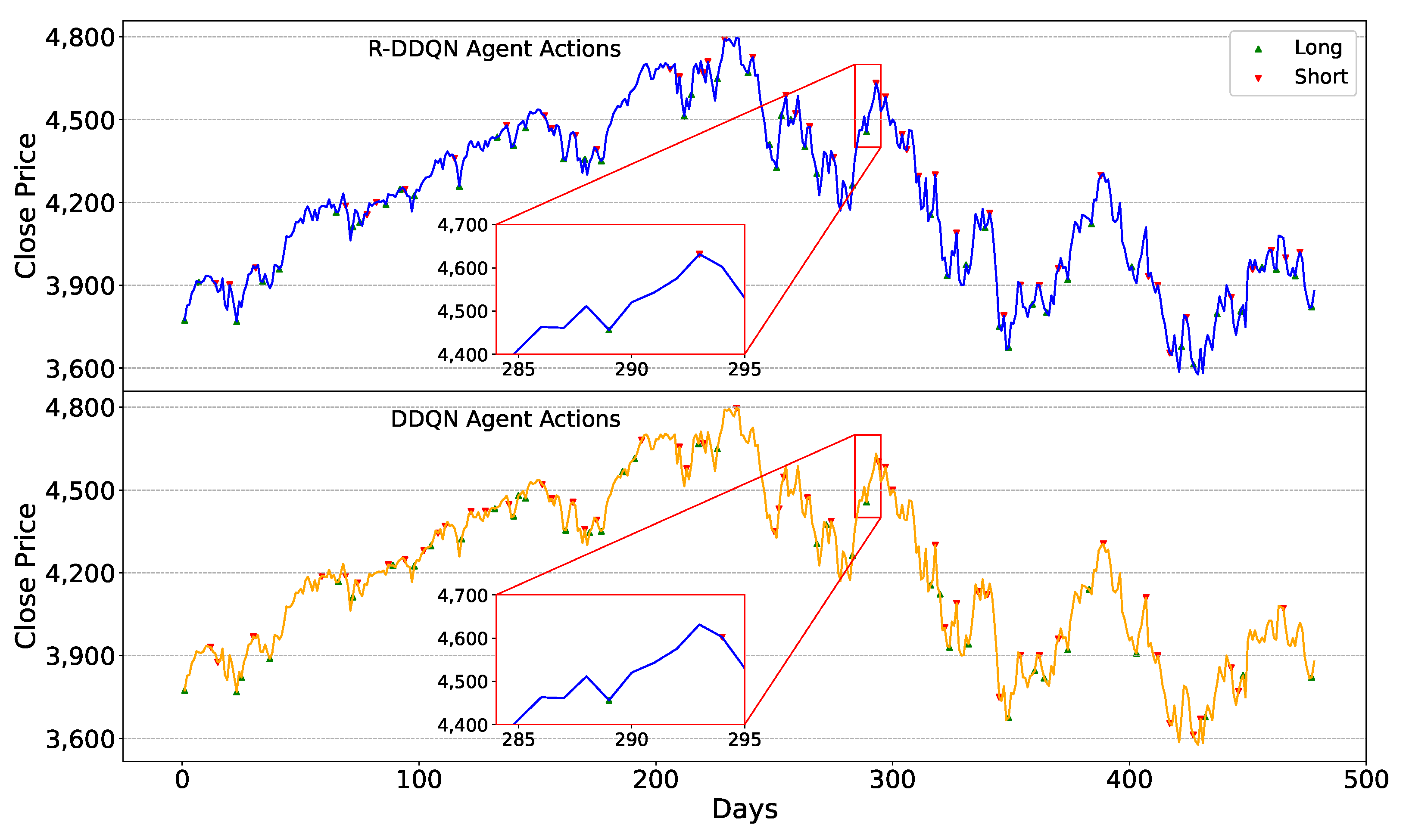
The trading strategies of the R-DDQN agent during the testing phase need to be analyzed, observing the trading decisions made amid continuous price fluctuations. Additionally, since R-DDQN is based on the DDQN algorithm, the trading decisions of R-DDQN and DDQN within the same timeframe also need to be compared. The trading strategies of the R-DDQN and DDQN agents on the six test sets are depicted in Figure 5, Figure 6, Figure 7, Figure 8, Figure 9 and Figure 10. Also, the number of transactions from R-DDQN and DDQN across six datasets is shown in

Table 6. The number of transactions from R-DDQN and DDQN across six datasets.

Datasets	Actions	R-DDQN	DDQN
HSI	Long	53	44
	Short	64	54
IXIC	Long	52	54
	Short	48	55
S&P500	Long	49	38
	Short	45	50
GOOGL	Long	60	51
	Short	54	52
MSFT	Long	61	64
	Short	60	61
INTC	Long	60	70
	Short	61	56

. From these figures, the following observations can be made:

Firstly, when facing the same market conditions, the R-DDQN agent can make more timely and accurate trading decisions compared to the DDQN agent. Observing the zoomed-in portion of Figure 5, around day 338, the stock price reached a low point, followed by an upward trend. During this period, the R-DDQN agent chose to buy stocks at the low point and sell at the subsequent high point, resulting in a profit. In contrast, the DDQN agent did not take any action at either the high or low points, only selling the stocks around day 348. This illustrates that R-DDQN can foresee future price movements clearly and execute correct and precise trading actions to generate profit. 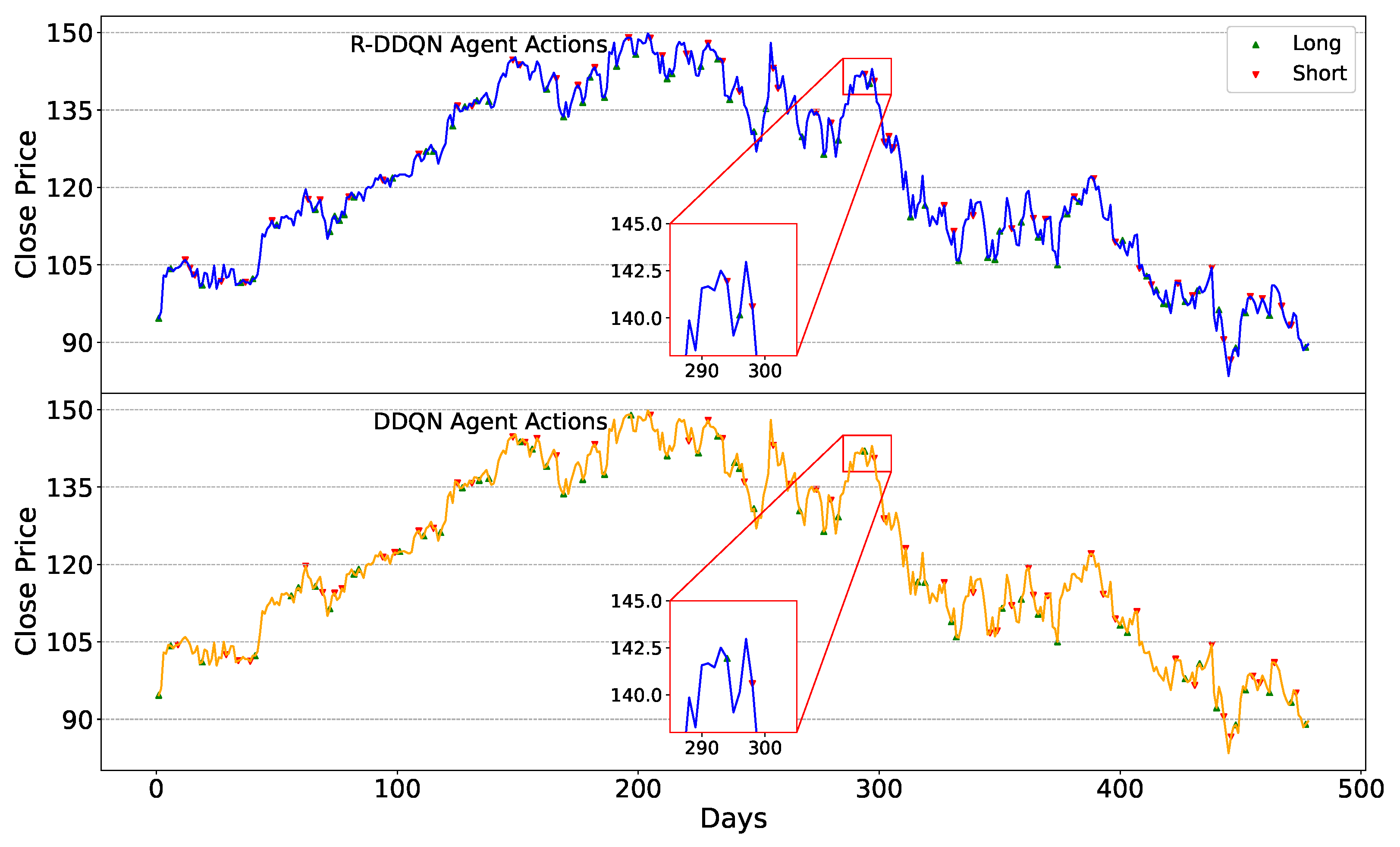Similar situations are also evident in Figure 6, where the price reached a peak around day 293, and R-DDQN sold stocks on that day while DDQN sold a day or two later.

Secondly, the reward function network of the R-DDQN agent is trained using pre-labeled expert demonstration data, while DDQN directly uses the equation that is used to label the example data as its reward function. However, when faced with the same market conditions and executing incorrect actions, the R-DDQN agent does not fall into the same predicament as the DDQN agent.

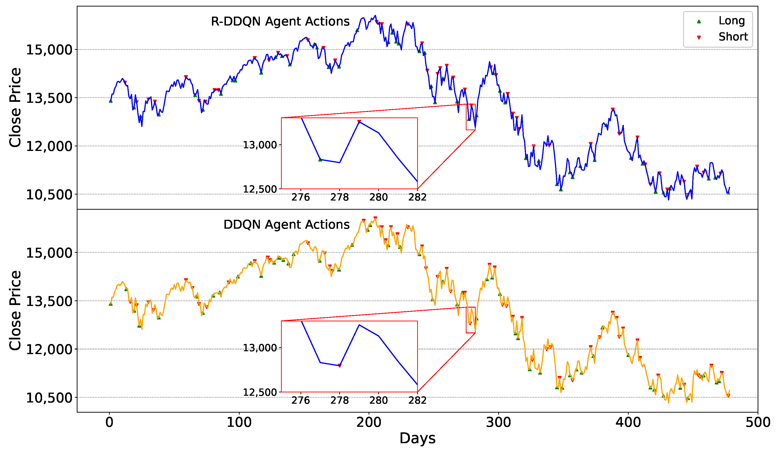
From the zoomed-in portion of Figure 9, it can be observed that during this period, the R-DDQN and the DDQN agents executed almost completely opposite trading actions. Similar situations are evident in Figure 7 and Figure 8. From the price movement curves, it is evident that the decisions made by the DDQN agent would undoubtedly lead to losses, while those made by the R-DDQN agent would result in profits.

This indicates that although the reward function network of R-DDQN is influenced by the DDQN reward function, the errors made by the DDQN agent are avoided by the R-DDQN agent. Conversely, when the DDQN agent incurs losses, the R-DDQN agent may generate profits. This demonstrates that the reward function network of the R-DDQN agent not only learns the reward generation patterns from expert demonstration data but also overcomes the shortcomings of the original reward function, enabling the agent to achieve greater returns.

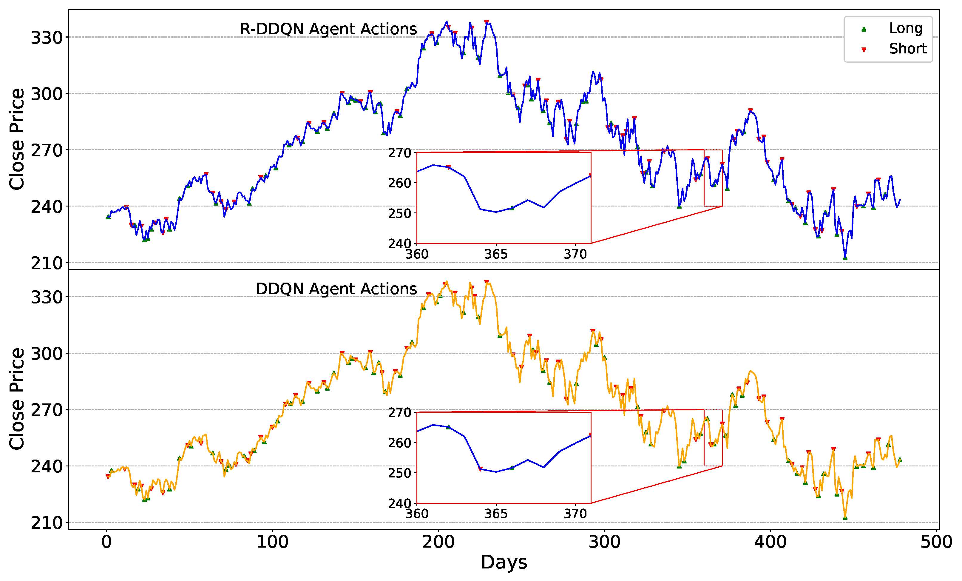
Finally, although the number of trading decisions from the R-DDQN agent shown in Table 6 is larger than that of the DDQN agent most of the time, the R-DDQN tends to execute fewer trading actions but achieves higher returns when potential risks arise. From Figure 10, it can be observed that from around day 405 to day 420, the stock price experienced a prolonged decline. During this period, the DDQN agent attempted multiple trading actions, some of which undoubtedly resulted in losses. However, the R-DDQN agent only sold stocks at the beginning of the decline and bought stocks at the end, resulting in profits with these trading decisions. From this, it is evident that R-DDQN not only accurately anticipates future stock price movements but also tends to execute trading actions efficiently. It avoids executing some trading decisions that may lead to losses or have little significance. Consequently, the performance of R-DDQN on multiple datasets surpasses that of DDQN.

4.7. Analysis with Short-Selling Costs

This section provides a comprehensive analysis of trading strategies by considering additional transaction costs based on the HSI and IXIC datasets. The following scenarios: R-DDQN (additional cost), R-DDQN (no cost), R-DDQN (no short), and the original R-DDQN are compared with the metrics mentioned above. Also, the quantity of trading actions (QTAs) is included as one of the metrics. The R-DDQN (additional cost) scenario includes a transaction cost of 0.3% per transaction and short-selling costs consisting of borrowing fees of $2/365\%$ per day and margin costs of 0.5% per transaction, reflecting the most realistic trading conditions. The R-DDQN (no cost) scenario does not consider any transaction or short-selling costs, providing an idealized performance benchmark. The R-DDQN (no short) scenario excludes short-selling, highlighting the impact of short-selling on performance. It is worth noting that R-DDQN (no short) still has a transaction cost of 0.3% per transaction. The original R-DDQN scenario does not include additional costs or short-selling restrictions for reference.

In

Table 7. The performance of R-DDQN in various trading mechanism scenarios across HSI and IXIC datasets.

Datasets	Metrics	B&H	R-DDQN (Additional Cost)	R-DDQN (No Cost)	R-DDQN (No Short)	R-DDQN
HSI	CR ↑	−5.51%	365.90%	1187.93%	128.73%	601.06%
	AR↑	−23.34%	117.84%	185.16%	66.57%	145.05%
	SR↑	−0.68	3.55	6.26	2.24	4.81
	MDD↓	45.38%	10.28%	3.60%	11.07%	8.95%
	QTA	1	108	121	75	117
IXIC	CR↑	−3.77%	491.90%	1099.82%	153.92%	790.00%
	AR↑	−12.38%	129.14%	173.63%	71.07%	154.76%
	SR↑	−0.33	4.22	6.09	2.89	5.55
	MDD↓	33.86%	3.53%	6.84%	10.58%	4.35%
	QTA	1	95	106	71	100

The bolded parts represent the best experimental results.

, the experiment results of the above scenarios along with B&H are presented. The introduction of additional transaction costs, especially short-selling costs, significantly affects the performance metrics. When no transaction costs are considered, the CR of R-DDQN increases, and the quantity of trading actions rises. For example, on the HSI dataset, the CR of R-DDQN increases from 601.06% to 1187.93%, and the quantity of trading actions rises from 117 to 121. However, with additional transaction costs, the CR drops to 365.90%, and the quantity of trading actions decreases to 108. Similarly, without the short-selling mechanism, the CR decreases to 128.73%, and the quantity of trading actions drops to 75. The same trend can be observed in the IXIC dataset. The reason for the significant change in CR with or without trading costs is that the saved trading costs can be used to purchase additional stocks. Therefore, when there are no trading costs, agents can obtain more stocks in a single “long” trading decision, resulting in greater profits when selling the held stocks.

The analysis shows that the proposed R-DDQN strategy still outperforms other baselines even after accounting for additional costs and short-selling mechanisms in a more realistic trading environment. In particular, for R-DDQN (no short), although short-selling is no longer permitted, it still achieves a better performance than B&H and other baselines. When there are no transaction costs, the cumulative return is higher, and the quantity of trading actions increases. When the short-selling mechanism is eliminated, the cumulative return is lower, and the quantity of trading actions decreases. When the cost of short-selling transactions is increased, the cumulative return is also lower, and the quantity of trading actions decreases. These experimental results further illustrate the effectiveness of our proposed method.

5. Discussion

The preceding sections provided a comprehensive analysis of R-DDQN. Across the testing results on six datasets, this method consistently outperformed several baseline models used for comparison. Moreover, in the analysis of trading strategies, the decision-making of the R-DDQN agent proved to be precise and judicious. From these experimental results, the following observations can be made:

Firstly, the reward function network of R-DDQN is trained specifically for different datasets. To further investigate its effectiveness, the concept of large models can be introduced. In future work, the reward function network can be trained on a large dataset that combines multiple stock indices and stocks, aiming to obtain a reward function network that accurately predicts reward values across different datasets. Recent studies have shown the significance of training agents with a large dataset. For example, Huang et al. [32] trained their proposed method in a mixed dataset that consist of multiple stock indices from the U.S. and then tested their results in multiple U.S. stocks. The experiment results showed that the cumulative return of their proposed method outperformed several baselines. In this case, the idea of incorporating a large dataset into DRL would enable a deeper exploration of the performance of R-DDQN.

Secondly, it is important to note that the expert sample data used to train the reward function network are labeled through a specific formula. Different labeling rules may result in varying performances for R-DDQN. Therefore, future work could involve comparing the performances of different expert sample data labeling rules across multiple datasets.

Thirdly, the data used to train the agent and the reward function network consist of daily and weekly data. Experimental results indicate that incorporating weekly data alongside the original daily data can significantly enhance the performance of the agent. This enhancement is attributed to providing the agent with a more diverse observation of stock market price movements, enabling the agent to extract more useful latent representations from the data. To be more specific, Kochliaridis et al. [40] built their dataset not only with OHLCV but also with lots of technical indicators like EMA (exponential moving average), DEMA (double-exponential moving average), and MACD (moving average convergence/divergence). The experimental results showed that their proposed method can have a significant performance when trading in the environment of cryptocurrencies. Therefore, future research could explore incorporating additional sources of information such as news or financial reports into the data to further enhance the model’s capabilities.

Fourthly, it is worth noting that the actual actions executed by the agent in the proposed method during trading are not entirely consistent with the trading signals generated by the policy network. The experiment we designed involves an “all-in” mechanism, and the actual actions executed are determined by combining the trading signals from the policy network with the current account positions. For example, if the policy network generates a buy signal for a long position but the account already holds a long position, it will hold the long position. For more detailed information, please refer to Table 1. However, the current trading mechanism is limited by the operation of full buy/sell orders and single-asset trades. Future work will focus on trading positions and slippage considerations.

Finally, the fundamental role of the reward function network is to replace the reward function in deep reinforcement learning algorithms. Therefore, it is promising to combine it with algorithms other than DDQN, such as PPO [41], A2C [42], and others.

6. Conclusions

In this paper, inspired by the reinforcement learning from human feedback (RLHF) concept and the double deep Q network (DDQN) algorithm, the reward-driven double DQN (R-DDQN) is proposed. This algorithm involves training a reward function network to replace the predefined reward function in deep reinforcement learning algorithms, aiming to enhance the performance of reinforcement learning agents in financial environments. By combining the reward function network with DDQN, a significant improvement in trading performance in the algorithmic trading area has been observed. Among all datasets, a maximum cumulative return of 1502% has been achieved during the testing phase. This paper makes the following contributions:

Firstly, a novel deep reinforcement learning framework built upon double DQN is introduced, which innovatively integrates the concept of RLHF. In this framework, a reward function network trained via supervised learning replaces the reward function in the DDQN algorithm. This substitution enables the DDQN agent to receive reward signals from the environment predicted by a neural network rather than being computed by a specific formula. Experimental results demonstrate a significant improvement in the performance of the agent in single-asset financial trading, with the proposed algorithm achieving the highest CR, AR, and SR across six datasets and maintaining optimal MDD in most cases. Consequently, this framework exhibits promising innovation and benefits in the field of financial trading.

Secondly, concerning the training of the reward function network, this paper employs cross-entropy to compute the loss when predicting rewards with the reward function network. Specifically, the task of training the reward function network is transformed into a classification task. Both the network’s outputs and expert sample data are passed through a softmax function to convert them into probabilities, and then the loss is calculated using cross-entropy. The experimental results indicate that this modification enhances the performance of the agent in trading activities.

Thirdly, the introduction of daily and weekly data undoubtedly leads to a significant improvement in the performance of the agent. The inclusion of weekly data provides the agent with a more diverse observation of stock market price movements and more extractable features. As a result, with the support of daily and weekly data, the agent achieves the highest CR across all six datasets.

Fourthly, further analysis with a more realistic trading condition, which considers the borrowing fees and margin cost to be the short-selling cost, is conducted with HSI and IXIC datasets. During the experiment, the CR of R-DDQN dropped significantly due to the additional cost but still had a better performance than baselines. Furthermore, an experiment in the scenario with no trading cost and no short-selling was also conducted. The experiment results showed that R-DDQN can achieve much higher CR when trading without any cost and has a relatively weak performance when short-selling is no longer available. In this case, the effectiveness of our proposed method has been well demonstrated.

Indeed, this research still has limitations. Firstly, the concept of the reward function network is only experimented with in the DDQN algorithm and has not been extended to other DRL algorithms. Secondly, the labeling rules for expert sample data are too singular, necessitating the introduction of different labeling rules to compare their performances. Thirdly, although daily and weekly data enhance the performance of the agent, it remains unexplored whether the introduction of more diverse data would further improve the agent’s performance. Fourthly, the current experiments and selected baselines are tailored for the U.S. stock market, where “short positions” are allowed. However, not all stock markets permit “short positions”, such as certain sectors of the Chinese stock market. Focusing solely on a single market would greatly reduce the generalizability of the proposed work. Therefore, future work should aim to incorporate stock or index data from the Chinese stock market as training datasets. Additionally, relevant works characterized by “no short selling” should be considered as baselines for comparison.

In subsequent work, the aforementioned limitations will be gradually addressed. The reward function network will be integrated with more DRL algorithms, and data containing more information will be used to train the agents. However, as discussed earlier, potential research is to construct a large-scale mixed dataset to train a reward function network that can meet the needs of multiple market scenarios. Looking back at the recent developments in the field of AI, there is an increasingly urgent demand from researchers for large-scale models or works incorporating the concept of large models. Various fields are hoping for tools that can meet diverse needs and adapt to complex environments. As an algorithm applied to financial trading decisions, the work proposed in this paper will introduce elements such as multi-modality data and additional financial information in the future to meet the requirements of a broader range of investors.