Inverse Scheme to Locally Determine Nonlinear Magnetic Material Properties: Numerical Case Study

Abstract

We are interested in the determination of the local nonlinear magnetic material behaviour in electrical steel sheets due to cutting and punching effects. For this purpose, the inverse problem has to be solved, where the objective function, which penalises the difference between the measured and the simulated magnetic flux density, has to be minimised under a constraint defined according to the corresponding partial differential equation model. We use the adjoint method to efficiently obtain the gradients of the objective function with respect to the material parameters. The optimisation algorithm is low-memory Broyden–Fletcher–Goldfarb–Shanno (BFGS), the forward and adjoint formulations are solved using the finite element (FE) method and the ill-posedness is handled via Tikhonov regularisation, in combination with the discrepancy principle. Realistic numerical case studies show promising results.

1. Introduction

For manufacturers of magnetic materials, measurement techniques are used to determine macroscopic properties in terms of characteristics (losses, magnetisation, coercive and remanent fields, etc.) and curves (virgin curve, hysteresis loop, commutation curve, etc.). In addition, these measurement techniques are used for the systematic study and development of materials. Many of the common test methods are specified in IEC 60404 ff. Standard techniques include the hysteresis graph, the coercive meter, the Epstein frame, the single sheet tester and the double-C yoke (see, for example, [1]).

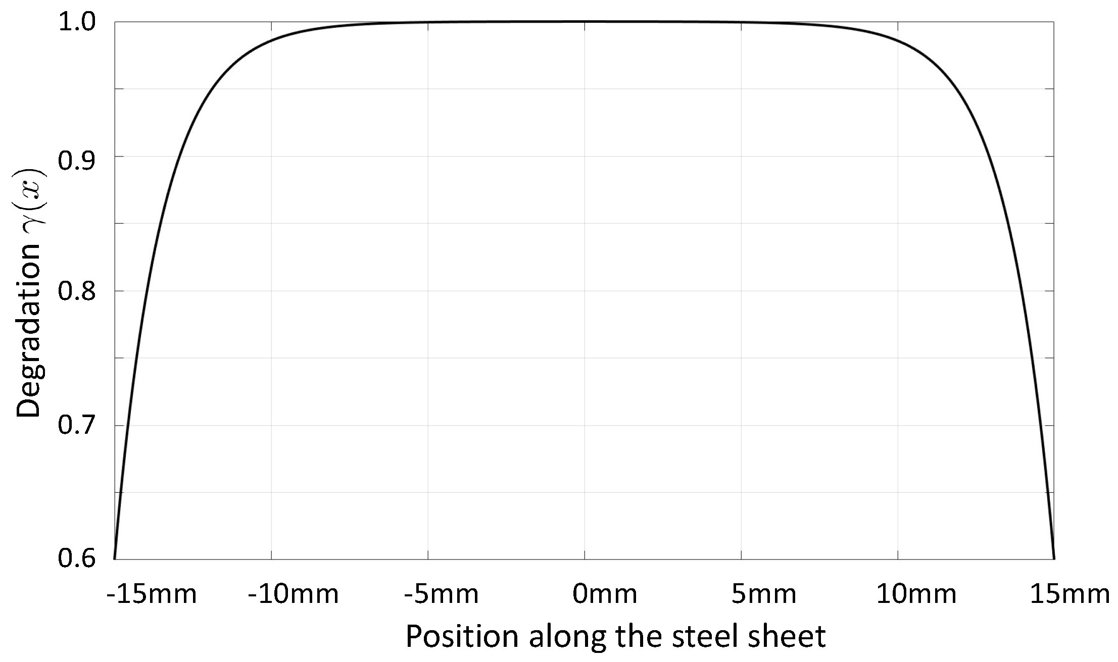
In order to better understand and model the various loss mechanisms that occur in electrical machines during operation, the actual degradation of electrical steel sheets due to cutting, punching, welding etc. is of paramount importance. A finite-element (FE) model has been presented in [2] in order to consider the local degradation effect. The approach introduces a certain number of boundary layers along the punched edges, where the relative permeability decreases according to a certain degradation profile. Thereby, the degradation profile has been assumed to be

$$\gamma \left(x\right)=1-\left(1-\widehat{\gamma }\right)e^{-x/\delta }$$

(1)

with an initial value $\widehat{\gamma }$ at the cut edge and the degradation skin depth $\delta$. Figure 1 displays such a degradation profile for $\widehat{\gamma }=0.6$ and $\delta =1.5$mm evaluated in [2].

In [3], the effects of three different cutting techniques, namely punching, waterjet and laser cutting, on the magnetic properties of grain-oriented electrical steel sheets have been investigated, and a loss model based on measurements (using an Epstein frame) has been developed. The result showed that the relative increase in core losses was in the range of 180–120%, 50–40% and $6\%$ for laser, punching and waterjet cutting, respectively. In addition to such approaches, measurements based on sensors that evaluate the magnetic field locally, e.g., in [4,5], have been developed. In [4], the needle probe method was used in combination with a scalar Preisach hysteresis operator in 2D FE simulations (based on the diffusion equation for the magnetic field intensity), and the Preisach distribution function was identified via least squares minimisation using the sequential programming method. In [5], the hysteresis properties of electrical steel sheets in the centre of the test material could be determined based on a single U-shaped yoke electromagnet, two Hall sensors (measuring the tangential surface fields) and a sensing coil around the yoke. Impressive research has recently been presented in [6], where pressure needle probes and micrometric giant magneto-resistance (GMR) sensors were mounted on each of the steel sheets in a laminated core. This allowed measurements to be made of the magnetic hysteresis curves for all the individual steel sheets (the averaged magnetic property for each individual steel sheet; no consideration of the cutting-edge effect). In conclusion, there is currently no method available to locally determine the degradation of electric steel sheets due to punching and/or cutting processes so that material models can be fitted and numerical simulations can be performed with sufficient accuracy. It should be noted that the problem at hand is quite complex, as one can only measure the magnetic field quantities outside the steel sheets, i.e., the stray field. Therefore, the local determination of the magnetic material behaviour requires the solution of an inverse problem.

In a previous publication [7], we demonstrated the successful identification of the nonlinear $BH$-curve (relation between magnetic induction, $\mathit{B}$, and magnetic field strength, $\mathit{H}$) based on Epstein frame measurements using (1) a combined Newton-type method with a full multigrid method as a linear solver (i.e., iterative regularisation via coarse discretisation) and (2) a nonlinear full multigrid method. The aim of our current research is to develop a combined method based on measurements, numerical simulations and inverse schemes to determine a sequence of nonlinear $BH$-curves to locally characterise the magnetic properties of electrical steel sheets and, thus, be able to quantify the cutting-edge effects. Recently, we have proposed an inverse scheme capable of locally determining the change in the linear magnetic property (the linear relationship between B and H via magnetic reluctance) due to the cutting-edge effects. The approach is based on a quasi-Newton method using Broyden’s update formula to compute the gradients of the objective function with respect to the local linear magnetic reluctivity [8]. In order to advance the practical relevance, this research paper extends the linear magnetic material model to a nonlinear one and uses the adjoint method (see, e.g., [9]) to compute the gradients of the searched-for parameters, which are the coefficients in all $BH$-curves. We would like to emphasise that the developed inverse scheme is capable of determining local material parameters in general as soon as the measurement setup can be accurately simulated using a physical model based on partial differential equations.

The remainder of the article is structured as follows. In Section 2, we define the problem and discuss the physical model of a sensor–actuator system with which the measurements will be made (in our tests, these measurements will be provided through numerical simulations). Next, Section 3 describes in detail the inverse scheme, including the formulation of the forward, as well as adjoint, problems, the computation of the gradient and the regularization. Section 4 presents the numerical results, and their detailed discussion is summarised in Section 5. Finally, we conclude and provide an outlook for the next research steps.

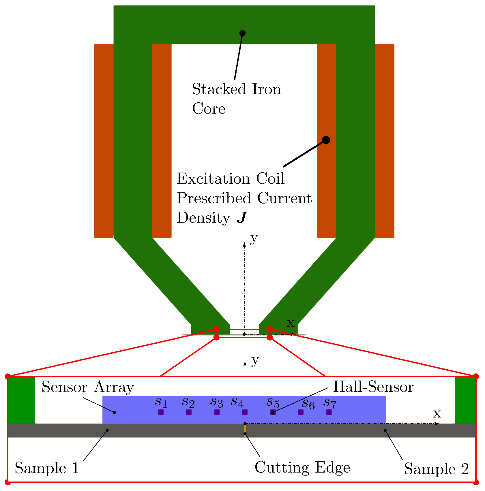
2. Problem Definition

We assumed an experimental setup displayed in Figure 2 and Figure 3.

The goal is to identify the nonlinear $BH$-curve in each subdomain ${\mathsf{\Omega }}_l$, especially to find out how the magnetic properties change in the direction of the cutting edges. In doing so, we assumed $N_{\mathrm{s}}$ sensors and $N_{\mathrm{p}}$ positions of the sensor–actuator system, and for each position, we excited the magnetic field from a minimum to a maximum over $N_{\mathrm{e}}$ excitation levels (the amplitude of the current density $\mathit{g}$). Therefore, the abstract problem may be defined as follows

$$\begin{array}{c}\hfill \underset{\mathit{u}\in V,\mathit{\theta }\in {\mathbb{R}}^{n_{\theta }}}{\min }J\left(\mathit{u},\mathit{\theta }\right)\mathrm{s}.\mathrm{t}.\mathcal{A}(\mathit{u},\mathit{\theta })=\mathbf{0}.\end{array}$$

(2)

In (2), the model operator $\mathcal{A}$ is defined according to the partial differential equation (PDE) of magnetostatics, which has to be solved in order to get the magnetic vector potentials, $\mathit{u}$, and in a postprocessing step, the magnetic flux densities, $\mathit{B}$ (for details, see Section 3.1). In doing so, the objective functional is defined according to

$$J\left(\mathit{u},\mathit{\theta }\right)=\frac{1}{2}\sum _{p=1}^{N_{\mathrm{p}}}\sum _{e=1}^{N_{\mathrm{e}}}\sum _{s=1}^{N_{\mathrm{s}}}\frac{1}{|{\mathsf{\Omega }}_s^{\mathrm{sens}}|}\underset{{\mathsf{\Omega }}_s^{\mathrm{sens}}}{\int }|{\mathit{B}}_{p,e,s}-{\mathit{B}}_{p,e,s}^{\mathrm{meas}}{|}^2\mathrm{d}\mathsf{\Omega }+\underset{\mathrm{regularization}\mathrm{term}}{\underbrace{\alpha {(\mathit{\theta }-{\mathit{\theta }}^{\mathrm{ref}})}^T\mathit{D}(\mathit{\theta }-{\mathit{\theta }}^{\mathrm{ref}})}},$$

(3)

where ${\mathsf{\Omega }}_s^{\mathrm{sens}}$ is the domain of sensor s, ${\mathit{B}}_{p,e,s}=\nabla \times {\mathit{u}}_{p,e,s}$ is the computed magnetic flux density and ${\mathit{B}}_{p,e,s}^{\mathrm{meas}}$ the measured one, ${\mathit{u}}_{p,e,s}$ the computed magnetic vector potential, $\mathit{\theta }=({\mathit{\theta }}_1,\dots ,{\mathit{\theta }}_{N_{\mathrm{sd}}})$ the vector of parameters of the $BH$-curves, ${\mathit{\theta }}^{\mathrm{ref}}$ the vector of reference parameters of the $BH$-curves and $\mathit{D}$ a diagonal weighting matrix. Since the entries in the parameter vector $\mathit{\theta }$ are of different sizes, the diagonal matrix $\mathit{D}$ scales them to a value of about $1.0$. Furthermore, $\mathcal{A}:V\times {\mathbb{R}}^{n_{\theta }}\to W$ is the model operator (defined according to the weak form of the PDE, including boundary conditions) with appropriate function spaces, V and W.

3. Inverse Scheme

Let us introduce the parameter-to-state map,

$$S:{\mathbb{R}}^{n_{\theta }}\to V\mathit{\theta }\to \mathit{u}\mathrm{s}.\mathrm{t}.\mathcal{A}(\mathit{u},\mathit{\theta })=0,$$

(4)

which is implicitly defined via the model equation

$$\mathcal{A}(S\left(\mathit{\theta }\right),\mathit{\theta })=0\mathrm{for}\mathrm{all}\mathit{\theta }\in {\mathbb{R}}^{n_{\theta }}.$$

(5)

The Lagrange function is introduced as

$$\mathcal{L}(\mathit{u},\mathit{\theta },\mathit{w})=J(\mathit{u},\mathit{\theta })+{〈\mathcal{A}(\mathit{u},\mathit{\theta }),\mathit{w}〉}_W,$$

(6)

where $<·,·{>}_W$ denotes the dual pairing between some function space, W, and its dual $W^{*}$. In the next step, the reduced objective function can be defined as follows

$$j\left(\mathit{\theta }\right)=J\left(\mathit{u}\right(\mathit{\theta }),\mathit{\theta })=\mathcal{L}\left(S\right(\mathit{\theta }),\mathit{\theta },\mathit{w}).$$

(7)

Assuming that the parameter to state map S is well defined, and $\mathcal{A},J,S$ are differentiable, we can express the partial derivatives of the reduced functional with reference to each parameter ${\theta }_i$ as

$$\begin{array}{ccc}\hfill \frac{\partial j}{\partial {\theta }_i}& =& \frac{\partial J}{\partial {\theta }_i}+{〈\frac{\partial J}{\partial \mathit{u}},\frac{\partial S}{\partial {\theta }_i}〉}_V+{〈\frac{\partial \mathcal{A}}{\partial \mathit{u}}\frac{\partial S}{\partial {\theta }_i},\mathit{w}〉}_W+{〈\frac{\partial \mathcal{A}}{\partial {\theta }_i},\mathit{w}〉}_W\hfill \end{array}$$

(8)

for any $\mathit{w}\in W$. Using the identity

$${〈\frac{\partial A}{\partial \mathit{u}}\frac{\partial S}{\partial {\theta }_i},\mathit{w}〉}_W={〈{\left(\frac{\partial A}{\partial \mathit{u}}\right)}^{*}\mathit{w},\frac{\partial S}{\partial {\theta }_i}〉}_V,$$

containing the adjoint operator defined according to

$$B^{*}:W^{*}\to V^{*}\mathrm{is}\mathrm{adjoint}\mathrm{to}B:V\to W\iff {\forall }_{\mathit{v}\in V,\mathit{w}\in W}:{〈B\mathit{v},\mathit{w}〉}_W={〈B^{*}\mathit{w},\mathit{v}〉}_V,$$

we obtain

$$\begin{array}{ccc}\hfill \frac{\partial j}{\partial {\theta }_i}& =& \frac{\partial J}{\partial {\theta }_i}+{〈\frac{\partial J}{\partial \mathit{u}}+{\left(\frac{\partial \mathcal{A}}{\partial \mathit{u}}\right)}^{*}\mathit{w},\frac{\partial S}{\partial {\theta }_i}〉}_V+{〈\frac{\partial \mathcal{A}}{\partial {\theta }_i},\mathit{w}〉}_W.\hfill \end{array}$$

(9)

Choosing $\mathit{w}$ such that it solves the adjoint equation

$${\left(\frac{\partial \mathcal{A}}{\partial \mathit{u}}\right)}^{*}\mathit{w}=-\frac{\partial J}{\partial \mathit{u}}$$

(10)

allows us to rewrite (8) as

$$\frac{\partial j}{\partial {\theta }_i}=\frac{\partial J}{\partial {\theta }_i}+{〈\frac{\partial \mathcal{A}}{\partial {\theta }_i},\mathit{w}〉}_W.$$

(11)

For the nonlinear $BH$-curve, we make the following nonlinear function ansatz:

$$H\left(B\right)=\nu \left(B\right)B=\left(c_0+c_1{B}^{c_2}\right)B$$

(12)

with constants $c_0$, $c_1$ and $c_2$ yet to be determined. The reluctivity is computed via

$$\nu \left(B\right)=c_0+c_1{B}^{c_2},$$

(13)

and its derivative via

$$\frac{\partial \nu }{\partial B}={\nu }^{\prime }\left(B\right)=c_1{c}_2{B}^{c_2-1}.$$

(14)

Since we assume a possibly different $\nu \left(B\right)$ curve in each of the $N_{\mathrm{sd}}$ subdomains (see Figure 3), we have $n_{\theta }=3N_{\mathrm{sd}}$ parameters to identify. In addition, the model operator describes the magnetostatic field

$$\mathcal{A}({\mathit{u}}_{p,e},\mathit{\theta })={\left(\nabla \times \left(\nu \left(B_{p,e}\right)\nabla \times {\mathit{u}}_{p,e}\right)-{\mathit{g}}_{p,e}\right)}_{\begin{array}{ccc}p\hfill & =\hfill & 1,\dots ,N_{\mathrm{p}}\hfill \\ e\hfill & =\hfill & 1,\dots ,N_{\mathrm{e}}\hfill \end{array}}$$

(15)

with

$${\nu }_l\left(B\right)=c_{0,l}+c_{1,l}{B}^{c_{2,l}}\mathrm{on}{\mathsf{\Omega }}_l;l=1,\dots ,N_{\mathrm{sd}}.$$

The weak form reads as

$$\begin{array}{cc}\hfill & 0=\underset{\mathsf{\Omega }}{\int }\left(\nu \left(B_{p,e}\right)\nabla \times {\mathit{u}}_{p,e}·\nabla \times \mathit{v}-{\mathit{g}}_{p,e}·\mathit{v}\right)\mathrm{d}{\mathsf{\Omega }}^{\prime }\mathrm{for}\mathrm{all}\mathit{v}\in W,\hfill \\ \hfill & p=1,\dots N_{\mathrm{p}}e=1,\dots N_{\mathrm{e}}\hfill \end{array}$$

(16)

with the function spaces $W=V\subseteq H_0\left(curl\right)$ [10]. The boundary condition included in the definition of the function spaces $W,V$ is $\mathit{u}\times \mathit{n}=0$, resulting in closed field lines corresponding to a solenoidal vector field.

3.1. Formulation of the Forward Problem

The sensors in the experimental setup shown in Figure 2 are Hall sensors capable of measuring static magnetic fields being generated via DC currents in the coils at different excitation levels. To solve the magnetic field problem according to (16), Newton’s scheme in the weak form for each sensor actuator position, p, and excitation level, e, reads as [10]

$$\begin{array}{c}\hfill \underset{\mathsf{\Omega }}{\int }\nu \left(B_{p,e}^k\right)\nabla \times \mathit{s}·\nabla \times {\mathit{v}}^{\prime }\mathrm{d}\mathsf{\Omega }+\underset{\mathsf{\Omega }}{\int }{\nu }^{\prime }\left(B_{p,e}^k\right)\nabla \times \mathit{s}·{\mathit{e}}_{B_{p,e}^k}{B}_{p,e}^k{\mathit{e}}_{B_{p,e}^k}·\nabla \times {\mathit{v}}^{\prime }\mathrm{d}\mathsf{\Omega }\\ \hfill =\underset{\mathsf{\Omega }}{\int }{\mathit{g}}_{p,e}·{\mathit{v}}^{\prime }\mathrm{d}\mathsf{\Omega }-\underset{\mathsf{\Omega }}{\int }\nu \left(B_{p,e}^k\right)\nabla \times {\mathit{u}}_{p,e}^k·\nabla \times {\mathit{v}}^{\prime }\mathrm{d}\mathsf{\Omega }\\ {\mathit{u}}_{p,e}^{k+1}={\mathit{u}}_{p,e}^k+\eta \mathit{s},\hfill \end{array}$$

(17)

where k is the iteration counter, and $\eta$ is some line search parameter determined using Armijo’s rule [11]. Edge finite elements are applied using basis functions and hierarchical polynomials from [12] to discretise the continuous $H_0\left(curl\right)$ function space. To ensure coercivity, a small regularisation parameter is used to scale the artificial mass matrix, whose entries are six orders of magnitude smaller than those of the stiffness matrix (for details, see [10]).

3.2. Formulation of the Adjoint Problem

Since $\mathcal{A}$ is self-adjoint, the left-hand side of (10) for each position, p, of the sensor–actuator system and excitation level, e, of the current density, $\mathit{g}$, in the coils is (see (18))

$$\begin{array}{ccc}\hfill 〈{\left(\frac{\partial \mathcal{A}}{\partial \mathit{u}}\right)}^{*}\left(S\left(\mathit{\theta }\right),\mathit{\theta }\right)\mathit{w},{\mathit{v}}^{\prime }〉& =& \underset{\mathsf{\Omega }}{\int }\nu \left(B_{p,e}\right)\nabla \times {\mathit{w}}_{p,e}·\nabla \times {\mathit{v}}^{\prime }\mathrm{d}\mathsf{\Omega }\hfill \\ & & +\underset{\mathsf{\Omega }}{\int }{\nu }^{\prime }\left(B_{p,e}\right)\nabla \times {\mathit{w}}_{p,e}·{\mathit{e}}_{B_{p,e}}{B}_{p,e}{\mathit{e}}_{B_{p,e}}·\nabla \times {\mathit{v}}^{\prime }\mathrm{d}\mathsf{\Omega }.\hfill \end{array}$$

(18)

For the right-hand side, we explore the Gâteaux derivative and obtain for each position, p, and excitation level, e,

$$\begin{array}{ccc}\hfill \underset{\epsilon \to 0}{\lim }\frac{1}{\epsilon }\left(J(\mathit{u}+\epsilon \mathit{v},\mathit{\theta })-J(\mathit{u},\mathit{\theta })\right)& =& \underset{\epsilon \to 0}{\lim }\frac{1}{2\epsilon }\sum _{s=1}^{N_{\mathrm{s}}}\frac{1}{|{\mathsf{\Omega }}_s^{\mathrm{sens}}|}\underset{{\mathsf{\Omega }}_s^{\mathrm{sens}}}{\int }({\left|\left({\mathit{B}}_{p,e,s}+\epsilon \nabla \times \mathit{v}\right)-{\mathit{B}}_{p,e,s}^{\mathrm{meas}}\right|}^2\hfill \\ & & -{\left|({\mathit{B}}_{p,e,s}-{\mathit{B}}_{p,e,s}^{\mathrm{meas}}\right|}^2)\mathrm{d}\mathsf{\Omega }\hfill \\ & =& \underset{\epsilon \to 0}{\lim }\frac{1}{2\epsilon }\sum _{s=1}^{N_{\mathrm{s}}}\frac{1}{|{\mathsf{\Omega }}_s^{\mathrm{sens}}|}\underset{{\mathsf{\Omega }}_s^{\mathrm{sens}}}{\int }(2\epsilon \left({\mathit{B}}_{p,e,s}-{\mathit{B}}_{p,e,s}^{\mathrm{meas}}\right)·\nabla \times \mathit{v}\hfill \\ & & +{\epsilon }^2 \nabla \times \mathit{v}·\nabla \times \mathit{v})\mathrm{d}\mathsf{\Omega }\hfill \\ & =& \sum _{s=1}^{N_{\mathrm{s}}}\frac{1}{|{\mathsf{\Omega }}_s^{\mathrm{sens}}|}\underset{{\mathsf{\Omega }}_s^{\mathrm{sens}}}{\int }\left({\mathit{B}}_{p,e,s}-{\mathit{B}}_{p,e,s}^{\mathrm{meas}}\right)·\nabla \times \mathit{v}\mathrm{d}\mathsf{\Omega }.\hfill \end{array}$$

(19)

and arrive at

$$-{〈\frac{\partial J}{\partial \mathit{u}},\mathit{v}〉}_{p,e}=\sum _{s=1}^{N_{\mathrm{s}}}\frac{1}{|{\mathsf{\Omega }}_s^{\mathrm{sens}}|}\underset{{\mathsf{\Omega }}_s^{\mathrm{sens}}}{\int }\left({\mathit{B}}_{p,e,s}^{\mathrm{meas}}-{\mathit{B}}_{p,e,s}\right)·\nabla \times \mathit{v}\mathrm{d}\mathsf{\Omega }.$$

(20)

Finally, the weak formulation for the adjoint equation reads as follows

$$\begin{array}{c}\hfill \underset{\mathsf{\Omega }}{\int }\nu \left(B_{p,e}\right)\nabla \times {\mathit{w}}_{p,e}·\nabla \times {\mathit{v}}^{\prime }\mathrm{d}\mathsf{\Omega }+\underset{\mathsf{\Omega }}{\int }{\nu }^{\prime }\left(B_{p,e}\right)\nabla \times {\mathit{w}}_{p,e}·{\mathit{e}}_{B_{p,e}}{B}_{p,e}{\mathit{e}}_{B_{p,e}}·\nabla \times {\mathit{v}}^{\prime }\mathrm{d}\mathsf{\Omega }\\ \hfill =\sum _{s=1}^{N_{\mathrm{s}}}\frac{1}{|{\mathsf{\Omega }}_s|}\underset{{\mathsf{\Omega }}_s}{\int }\left(\left({\mathit{B}}_{p,e,s}^{\mathrm{meas}}-{\mathit{B}}_{p,e,s}\right)·\nabla \times \mathit{v}\right)\mathrm{d}\mathsf{\Omega }.\end{array}$$

(21)

Note that the adjoint equation is linear and, therefore, extremely fast to solve compared to the forward simulation, which has to solve a nonlinear system of equations for all unknown vector potentials in the computational mesh (see (18)).

3.3. Computation of the Gradient

For the evaluation of the gradients, the first term in (11), according to (3), computes as

$$\frac{\partial J}{\partial \mathit{\theta }}=\alpha \mathit{D}\left(\mathit{\theta }-{\mathit{\theta }}^{\mathrm{ref}}\right).$$

(22)

The second term in (11) with the solution $\mathit{u}$ of the forward Problem (18) (note that $\mathit{B}=\nabla \times \mathit{u}$) and the solution $\mathit{w}$ of the adjoint Equation (21) is calculated according to

$$\begin{array}{ccc}\hfill 〈\frac{\partial \mathcal{A}}{\partial {\theta }_l}(\mathit{u},\mathit{\theta }),\mathit{w}〉& =& \sum _{p=1}^{N_{\mathrm{p}}}\sum _{e=1}^{N_{\mathrm{e}}}\underset{\mathsf{\Omega }}{\int }\frac{\partial \nu \left(B_{p,e}\right)}{\partial {\theta }_l}{\mathit{B}}_{p,e}·\nabla \times {\mathit{w}}_{p,e}\mathrm{d}{\mathsf{\Omega }}^{\prime }\hfill \\ \hfill l=1,\dots 3N_{\mathrm{sd}}\end{array}$$

(23)

The derivative of the magnetic reluctivity $\nu$ with reference to the coefficients in (23) is computed for each subdomain ${\mathsf{\Omega }}_l$ according to the chosen ansatz (13) via

$$\begin{array}{c}\hfill \frac{\partial \nu }{\partial c_{0l}}=1;\frac{\partial \nu }{\partial c_{1l}}=B^{c_{2l}};\frac{\partial \nu }{\partial c_{2l}}=c_{1l}\left(lnB\right)B^{c_{2l}}.\end{array}$$

(24)

3.4. Overall Inverse Scheme

According to the derivations in Section 3.1, Section 3.2 and Section 3.3, all components are available for the inverse scheme. Since the parameter vector $\mathit{\theta }$ is improved iteratively, a stopping criterion and a strategy for the regularisation parameter $\alpha$ in the objective function (3) are needed. To this end, the following relative $L_2$ error norm is defined:

$$\epsilon =\sqrt{\frac{{\displaystyle \sum _{p=1}^{N_{\mathrm{p}}}}{\displaystyle \sum _{e=1}^{N_{\mathrm{e}}}}{\displaystyle \sum _{s=1}^{N_{\mathrm{s}}}}|{\mathit{B}}_{p,e,s}-{\mathit{B}}_{p,e,s}^{\mathrm{meas}}{|}^2}{{\displaystyle \sum _{p=1}^{N_{\mathrm{p}}}}{\displaystyle \sum _{e=1}^{N_{\mathrm{e}}}}{\displaystyle \sum _{s=1}^{N_{\mathrm{s}}}}|{\mathit{B}}_{p,e,s}^{\mathrm{meas}}{|}^2}}.$$

(25)

In addition, the choice of the regularisation parameter is crucial in obtaining an optimal solution during the iterative process. If the regularisation parameter is set too high, the minimisation will prioritise the regularisation term, resulting in a strong bias, while setting it too low can lead to instability and the divergence of the iterative process. Depending on the accuracy and resolution of the sensors, there is an a priori upper bound $\beta$ for the error norm defined in (25) with ${\mathit{B}}_{p,e,s}={\mathit{B}}_{p,e,s}^{\mathrm{exact}}$. Using the discrepancy principle [13], an initial regularisation parameter ${\alpha }_{\mathrm{init}}$ is chosen, and it is reduced at each iteration step via

$${\alpha }_k=a^k{\alpha }_{\mathrm{init}}$$

(26)

until (25) with ${\mathit{B}}_{p,e,s}={\mathit{B}}_{p,e,s}^{\mathrm{comp}}$ is smaller than $\beta ={\epsilon }^{\mathrm{stop}}$. In all of the following calculations, the values $a=0.9$ and ${\alpha }_{\mathrm{init}}=10$ were chosen.

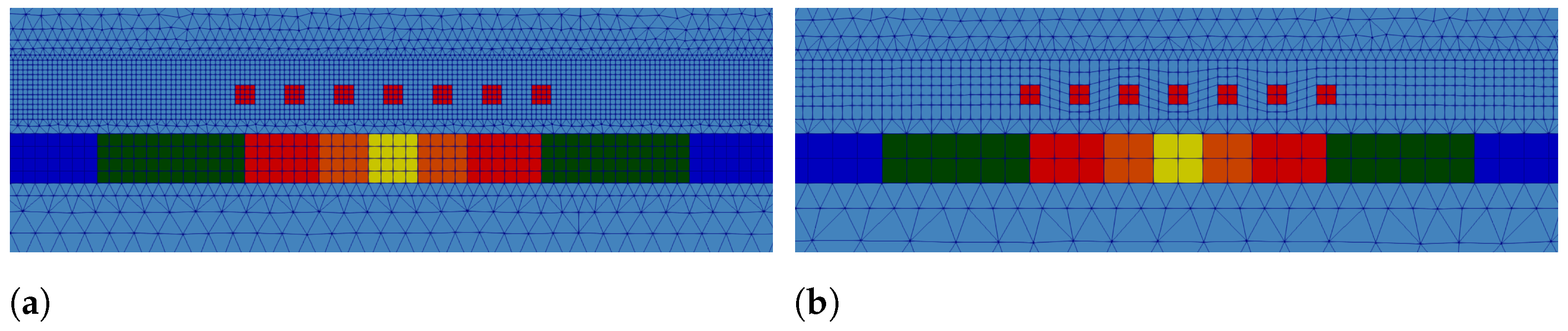
4. Numerical Results

Cutting electric steel sheets causes a severe degradation of the magnetic properties in the immediate vicinity of the cut edges. For this reason, the $0.5$mm-thick electrical steel sheets are divided into five subregions (see Figure 3), and the density of the regions is significantly higher due to the strong material gradient in the immediate vicinity of the cut edges. The affected region is assumed to have a total length, $x_{\mathrm{CE}}$, of 3 mm, and the lengths, $\Delta x_l$, of the respective subregions, ${\mathsf{\Omega }}_l$, are summarised in

Table 1. Length $\Delta x_l$ for each subdomain ${\mathsf{\Omega }}_l$.

	${\mathbf{\Omega }}_1$	${\mathbf{\Omega }}_2$	${\mathbf{\Omega }}_3$	${\mathbf{\Omega }}_4$	${\mathbf{\Omega }}_5$
$\Delta$x in mm	0.25	0.5	0.75	1.5	13

. This distribution of subdomains means that ${\mathsf{\Omega }}_5$ represents the bulk material (unaffected by cutting-edge effects), and it is assumed that the material data for this subdomain are already known from corresponding measurements with an Epstein frame or a single-sheet tester (SST).

The sensor–actuator system is equipped with $N_{\mathrm{s}}=7$ Hall sensors evenly distributed along the straight line $\left[\right(-1.5,0.4,0),(1.5,0.4,0\left)\right]$ in mm. The Hall sensors are capable of directly measuring all three spatial components of the stray field ($B_x$, $B_y$, $B_z$). The electrical steel sheet is measured at $N_{\mathrm{p}}=5$ different positions so that the Hall sensor $s_4$ (see Figure 2) is once directly over the cutting edge and once over the centre of each of the subdomains. Since the material behaviour of the two sheets is symmetrical, only the subdomains in the positive x-domain are measured. The resulting positions are $x_{\mathrm{p}}=\left[0,0.125,0.5,1.125,2.25\right]$ in mm, where $x_{\mathrm{p}}$ is the x-position of sensor $s_4$. At each position $N_{\mathrm{p}}$, the sheets are magnetised at $N_{\mathrm{e}}=15$ excitation levels by varying the current density, $\mathit{g}$, of the excitation coils. The different current density levels, $\mathit{g}\left(e\right)$, are defined according to the following relations

$$\mathit{g}\left(e\right)={\mathit{g}}_{\mathrm{init}}{10}^e,$$

(27)

where $|{\mathit{g}}_{\mathrm{init}}|=10,000\mathrm{A}/{\mathrm{m}}^2$ is the initial current density and $e=0.1,0.2,...,1.5$ the excitation levels.

Each subdomain is associated with a nonlinear magnetic material behaviour according to (12), where the parameters $c_0$, $c_1$ and $c_2$ are the unknowns to be determined in the inverse scheme. Since ${\mathsf{\Omega }}_5$ is the already-known bulk material, 12 unknown parameters must be determined $\mathit{\theta }=\left[{\theta }_{l,i}\right]$, where $l=1,2,3,4$ is the corresponding subdomain, and $i=0,1,2$ is the parameter index. For example, ${\theta }_{1,0}$ is the material parameter, $c_0$, of the subdomain ${\mathsf{\Omega }}_1$. 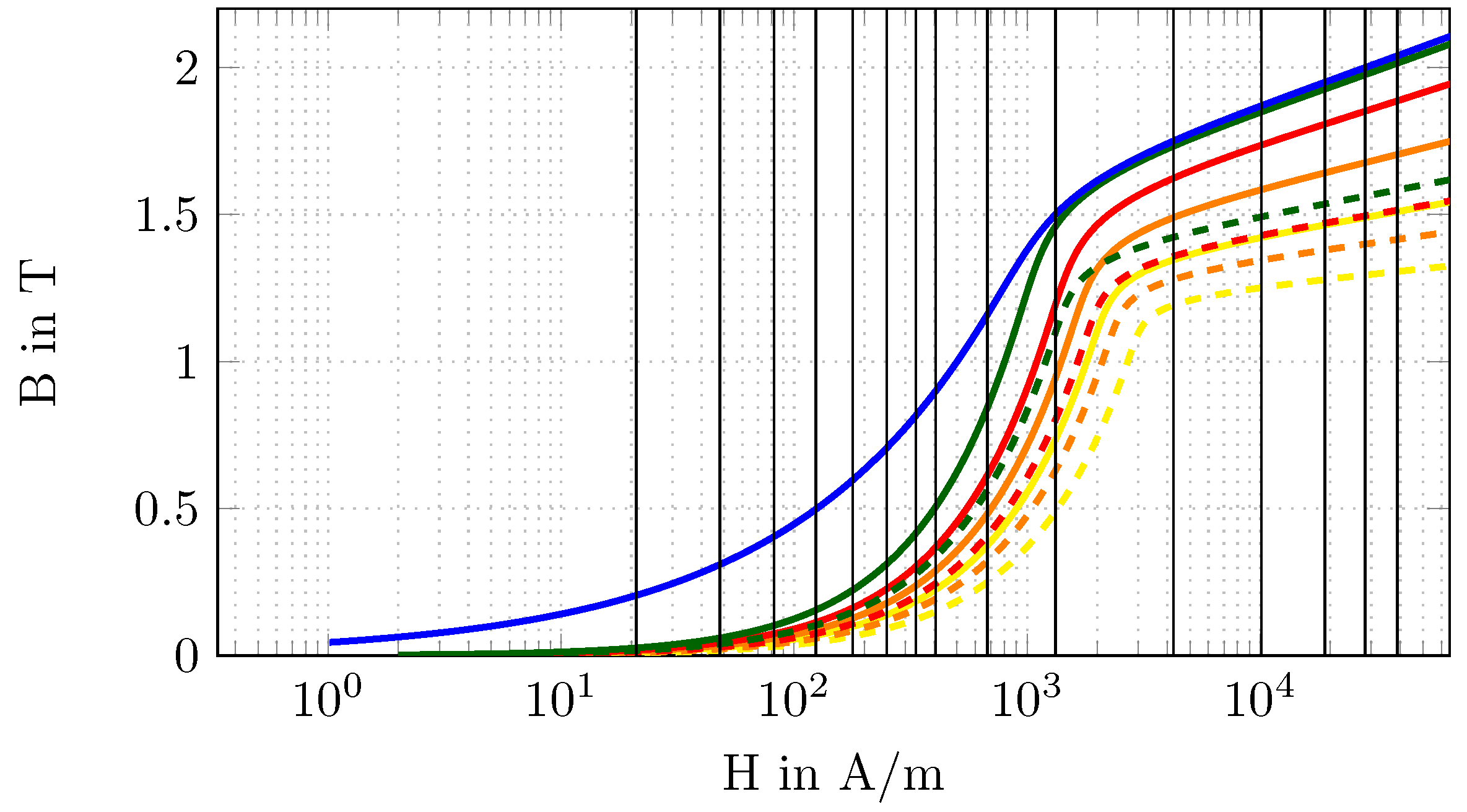For the numerical study, the parameters of the nonlinear material function, ${\nu }_l$, are classified into three cases, ${\nu }_l^{\mathrm{exact}}$, ${\nu }_l^{\mathrm{init}}$ and ${\nu }_l^{\mathrm{ref}}$. Thereby, ${\nu }_l^{\mathrm{exact}}$ defines the theoretically real material behaviour and serves as a reference in the sense of calculating the relative errors between the optimised ${\nu }_l^{\mathrm{opt}}$ and the exact parameters. Furthermore, ${\nu }_l^{\mathrm{init}}$ is the initial configuration for the iterative inverse scheme, and it has a $50\%$ deviation from the real configuration, ${\nu }_l^{\mathrm{exact}}$. In addition, ${\nu }_l^{\mathrm{ref}}$ is the reference configuration used for the Tikhonov regularisation, and it is here chosen as the arithmetic mean between ${\nu }_l^{\mathrm{init}}$ and ${\nu }_l^{\mathrm{exact}}$. The parameters for the different cases are listed in

Table 2. Parameters $c_0$, $c_1$ and $c_2$ for initial ${\nu }_l^{\mathrm{init}}$, reference ${\nu }_l^{\mathrm{ref}}$ and exact ${\nu }_l^{\mathrm{exact}}$ nonlinear reluctivity.

		${\mathit{\theta }}^{\mathbf{init}}$			${\mathit{\theta }}^{\mathbf{ref}}$			${\mathit{\theta }}^{\mathbf{exact}}$
Subdomain	Colour Code	${\mathit{c}}_{\mathbf{0}}$	${\mathit{c}}_{\mathbf{1}}$	${\mathit{c}}_{\mathbf{2}}$	${\mathit{c}}_{\mathbf{0}}$	${\mathit{c}}_{\mathbf{1}}$	${\mathit{c}}_{\mathbf{2}}$	${\mathit{c}}_{\mathbf{0}}$	${\mathit{c}}_{\mathbf{1}}$	${\mathit{c}}_{\mathbf{2}}$
${\mathsf{\Omega }}_1$		2700	1.2	37.5	2250	1.0	31.25	1800	0.8	25
${\mathsf{\Omega }}_2$		2100	0.75	30.0	1750	0.625	25.0	1400	0.5	20
${\mathsf{\Omega }}_3$		1650	0.6	25.5	1375	0.5	21.25	1100	0.4	17
${\mathsf{\Omega }}_4$		1200	0.375	24.0	1000	0.3125	20.0	800	0.25	16
${\mathsf{\Omega }}_5$		-	-	-	-	-	-	500	0.2	15

. The representative $BH$-curve for ${\nu }_l^{\mathrm{exact}}$ and ${\nu }_l^{\mathrm{init}}$ is shown in Figure 4.

The measured data, ${\mathit{B}}^{\mathrm{meas}}$, are generated by artificially applying the forward simulation with the exact material data, ${\nu }_l^{\mathrm{exact}}$, as listed in Table 2, and the defined excitation levels (see (27)). The measurements are taken at the previously defined positions. Thereby, measurement noise (Gaussian white noise, $\mathcal{N}(0,{\sigma }^2)$ with $\sigma =10\%$) is superimposed on the resulting data. To avoid an inverse crime, a finer computational grid of the sensor–actuator system was used to generate the measurement data compared to the model for the inverse scheme (see Figure 5).

The stopping criterion, ${\epsilon }^{\mathrm{stop}}$, for the iterative procedure can be determined a priori. To do this, the FE model for the inverse method (Figure 5b) is used to calculate the magnetic flux density, $\mathit{B}$, based on the exact material data, ${\nu }_l^{\mathrm{exact}}$. Here, we carried out a mesh independence study to obtain reliable magnetic flux density data at the sensor position, resulting in a mesh of approximately 100,000 unknowns (82,000 hexahedral and wedge elements). Based on these results and the previously simulated measurement data ${\mathit{B}}^{\mathrm{meas}}$ on the fine grid (see Figure 5a) superimposed by Gaussian noise with $\sigma =10\%$, the stopping value according to (25) gives ${\epsilon }^{\mathrm{stop}}=0.1023$. The optimisation algorithm is a low-storage BFGS from the NLopt software library [14], to which the computed gradient (11) and the relative $L_2$ error norm (25) are passed at each iteration step. In addition to the stopping criterion, a relative error $|\Delta {\mathit{\theta }}_k|/|{\mathit{\theta }}_k|<{\theta }_{\mathrm{tol}\_\mathrm{rel}}=0.001$ and a relative residual $\Delta {\epsilon }_k/{\epsilon }_k<{\epsilon }_{\mathrm{tol}\_\mathrm{rel}}=0.001$ are specified to allow the early termination of the optimisation if no further improvements are achieved.

Based on the given data, the sought parameter vector, $\mathit{\theta }$, is calculated using the proposed method, and the results are presented below. The optimisation was stopped after 48 iterations with a remaining relative error of $\epsilon =0.1048$. Since the specified stopping value, ${\epsilon }^{\mathrm{stop}}=0.1023$, could not be reached, the additionally defined tolerances, ${\theta }_{\mathrm{tol}\_\mathrm{rel}}$ and ${\epsilon }_{\mathrm{tol}\_\mathrm{rel}}$, were applied. 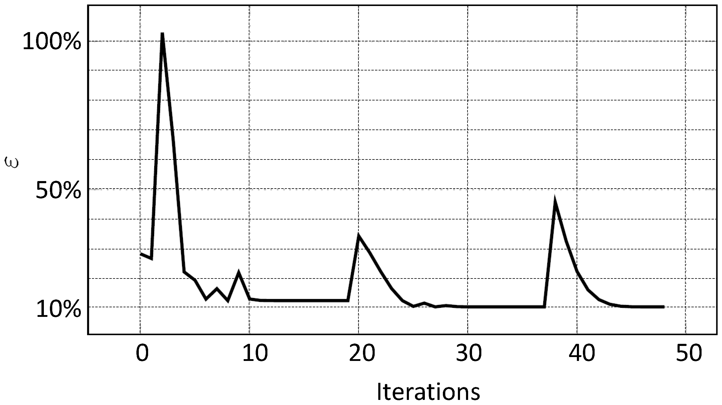The relative error of the unknown parameter vector, $\mathit{\theta }$, in each iteration step is shown in Figure 6 and the general convergence behaviour of the relative $L_2$ error $\epsilon$ in Figure 7.

The optimised values, ${\mathit{\theta }}^{\mathrm{opt}}$, and the relative errors, ${\theta }_{l,i}^{\mathrm{rel}}=|{\theta }_{l,i}^{\mathrm{opt}}-{\theta }_{l,i}^{\mathrm{exact}}|/|{\theta }_{l,i}^{\mathrm{exact}}|$, are listed in

Table 3. Optimised parameter, ${\mathit{\theta }}^{\mathrm{opt}}$, and relative error, ${\theta }^{\mathrm{rel}}$.

	${\mathit{\theta }}^{\mathbf{opt}}$			${\mathit{\theta }}^{\mathbf{rel}}$ in %
Subdomain	${\mathit{c}}_{\mathbf{0}}$	${\mathit{c}}_{\mathbf{1}}$	${\mathit{c}}_{\mathbf{2}}$	${\mathit{c}}_{\mathbf{0}}$	${\mathit{c}}_{\mathbf{1}}$	${\mathit{c}}_{\mathbf{2}}$
${\mathsf{\Omega }}_1$	1898.4	0.79	25.75	5.47	0.95	2.99
${\mathsf{\Omega }}_2$	1469.9	0.48	20.44	4.99	4.49	2.17
${\mathsf{\Omega }}_3$	1160.7	0.41	17.82	5.52	1.70	4.81
${\mathsf{\Omega }}_4$	876.9	0.20	16.99	9.62	19.73	6.18

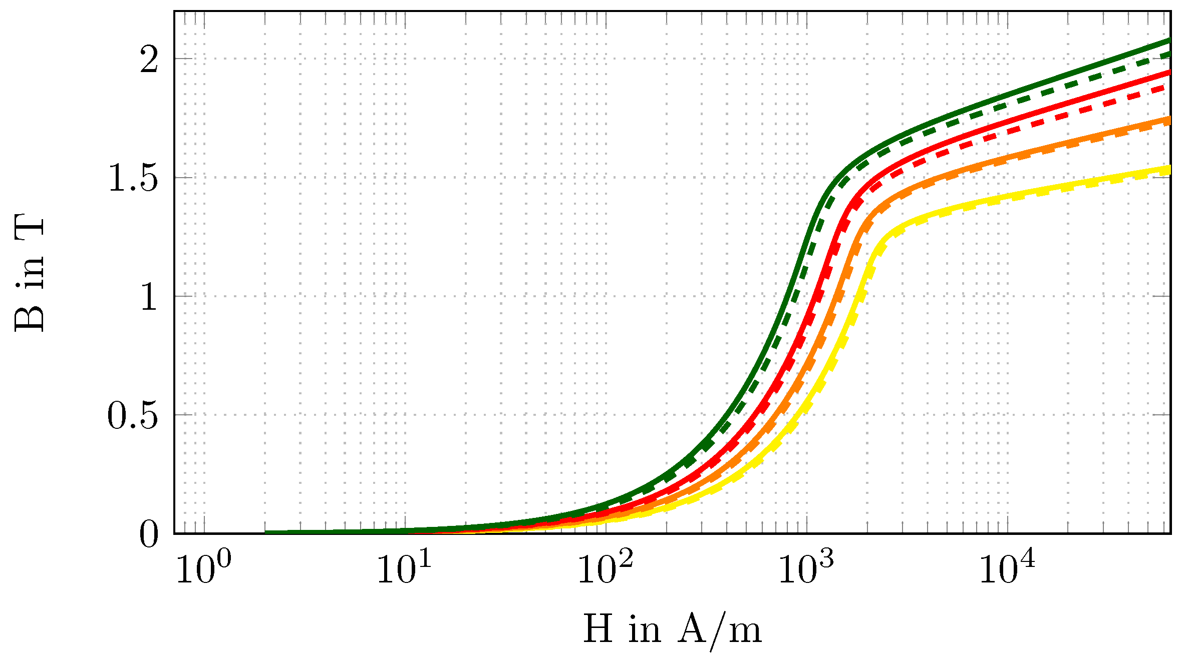
. The corresponding $BH$-curves are compared in Figure 8 to better illustrate the difference between the optimised parameters, ${\mathit{\theta }}^{\mathrm{opt}}$, and the exact parameters, ${\mathit{\theta }}^{\mathrm{exact}}$.

Finally, we would like to emphasise that the computational grid used for the inverse scheme resulted in about 39,000 unknowns (30,000 hexahedral and wedge elements), and the total time for obtaining the results (all 48 iterations, see Figure 7) was $2$h on a PC with 64 GB of memory (10 GB were used for the computation) and five cores. The computation for one FE solution of the nonlinear magnetostatic PDE needed about $1.5$ min. This clearly demonstrates the efficiency of the developed inverse scheme. In addition, the scheme does not rely on the low-storage BFGS, and other optimisers are being tested. The computation of the forward and adjoint problem was performed with the open-source FE solver software openCFS [15].

5. Discussion

The convergence behaviour of $\epsilon$ in Figure 7 shows two characteristic peaks at iteration steps 20 and 38, preceded by a region of barely noticeable change from the residual. These anomalies are also reflected in the behaviour of the relative parameter error, ${\theta }_{l,i}^{\mathrm{rel}}$, in Figure 6. For the iteration range between 12 and 19, there were no more significant changes in the parameters, although the parameters ${\theta }_{1,1}$ and ${\theta }_{4,1}$ still showed pronounced errors. The same can be observed for the iteration range of 30 to 37, with the exception that only the parameter ${\theta }_{4,1}$ shows increased deviations. Due to the underlying nonlinear problem, these anomalies indicate local minima where the optimisation procedure gets stuck and, therefore, there is no improvement in the relative $L_2$ error or the relative error of the parameters ${\theta }_{l,i}^{\mathrm{rel}}$. To overcome these local minima, the optimiser makes a significant change to the parameters, which is reflected in the subsequent deviation of the parameters. Thus, after iteration step 20, the relative error of the parameters ${\theta }_{1,1}$ and ${\theta }_{4,1}$ can be significantly improved. After iteration step 38, however, this did not lead to success, so the optimisation was stopped according to the additionally defined stopping criteria, although the predefined ${\epsilon }^{\mathrm{stop}}$ was not reached.

Comparing the $BH$-curves of the exact and optimised parameters, as shown in Figure 8, it can be seen that the curves based on the optimised parameter are lower than those based on the exact parameter. This behaviour is mainly due to the following points. Firstly, the measurement data used are superimposed with Gaussian white noise, which allows a solution to be found only in the vicinity of the exact solution. Secondly, due to the ill-posedness of the inverse problem and the consequent need to use a regularisation (Tikhonov regularisation), the regularisation term and, thus, the a priori information are included in the calculated parameters. This results in the remaining deviations listed in Table 3. However, the increased relative errors, ${\theta }_{l,i}^{\mathrm{rel}}$, for the subdomain ${\mathsf{\Omega }}_4$ are noteworthy. This could be due to the chosen excitation levels or the positioning of the sensor–actuator system in the sense that the sensitivity to the parameters in this subdomain is less pronounced compared to the others. These parameters were chosen arbitrarily. In order to use the optimal excitation levels and positioning of the sensor–actuator system with respect to the determination of the unknown material parameter vector $\mathit{\theta }$, a design of experiment (DOE) can significantly improve the current convergence behaviour.

6. Conclusions

In this research, we have presented an inverse scheme capable of determining the nonlinear magnetic material properties locally in the vicinity of the cut edges of electrical steel sheets. The approach was based on FE simulations of the magnetostatic field using the magnetic vector potential, $\mathit{u}$, and it locally identifies the magnetic reluctance as a function of the magnetic flux density, $\mathit{B}$. The objective function, which penalises the difference between the measured and simulated magnetic flux densities, is minimised under a constraint defined according to the corresponding partial differential equation for the magnetic vector potential. To efficiently obtain the gradients of the objective function with respect to the material parameters, the adjoint method is applied. The optimisation algorithm is a low-memory BFGS from the NLopt software library, the forward and adjoint formulations are solved using the open source FE solver openCFS [15], and the ill-posedness is handled via Tikhonov regularisation, in combination with the discrepancy principle. The numerical tests show promising results, and in future work, we will build the sensor–actuator system to perform real measurements and apply the developed inverse scheme to these data.