Article

Statistical Modeling of Right-Censored Spatial Data Using Gaussian Random Fields

by
Fathima Z. Sainul Abdeen
1,
Akim Adekpedjou
1,* and
Sophie Dabo Niang
2
1
Department of Mathematics and Statistics, Missouri University of Science and Technology, Rolla, MO 65409, USA
2
Laboratoire Paul Painvelé UMR CNRS 8524, INRIA-MODAL, University of Lille, F-59000 Lille, France
*
Author to whom correspondence should be addressed.
Mathematics 2024, 12(10), 1521; https://doi.org/10.3390/math12101521
Submission received: 9 April 2024 / Revised: 23 April 2024 / Accepted: 28 April 2024 / Published: 13 May 2024
(This article belongs to the Special Issue Clustered Data Modeling and Statistical Meta-Analysis)

Abstract

:
Consider a fixed number of clustered areas identified by their geographical coordinates that are monitored for the occurrences of an event such as a pandemic, epidemic, or migration. Data collected on units at all areas include covariates and environmental factors. We apply a probit transformation to the time to event and embed an isotropic spatial correlation function into our models for better modeling as compared to existing methodologies that use frailty or copula. Composite likelihood technique is employed for the construction of a multivariate Gaussian random field that preserves the spatial correlation function. The data are analyzed using counting process and geostatistical formulation that led to a class of weighted pairwise semiparametric estimating functions. The estimators of model parameters are shown to be consistent and asymptotically normally distributed under infill-type asymptotic spatial statistics. Detailed small sample numerical studies that are in agreement with theoretical results are provided. The foregoing procedures are applied to the leukemia survival data in Northeast England. A comparison to existing methodologies provides improvement.

1. Introduction

Right censored data are encountered in various settings such as biomedicine, reliability, actuarial science, sociology, politics, and public health, to name a few. They are part of a class of data called survival or failure time data, which include, among others, left and right censored, left and right truncation, and interval censored data. Research with these types of data is well documented. This manuscript pertains to another aspect of failure time data, namely one where spatial modeling is incorporated via geostatistical locations of units of interest. Consider the situation where these units, located at areas described by their longitude and latitude in a two-dimensional surface, are monitored for the occurrence of some event, such as the onset of a disease, an epidemic, claims filed as a result of property losses, cancer, or migration of individuals from one area to another to seek better living conditions. There exist environmental factors, social and physical environments, population density, or weather conditions beyond the control of the investigators that can have a substantial impact on the occurrence of events between two areas via their spatial coordinates. We give one example of such data in biomedical studies that will be used in the application section. Many more examples can be found in [1].
Example 1. 
Leukemia survival data: [2,3].
A total of 1043 adults were diagnosed with leukemia between 1982 and 1998, in Northeast England, which comprises 24 administrative districts boxed in 100 k m 2 . The data holds records of incidence and subsequent survival status of all leukemia cases in the region. Also recorded was the background variation in population or environmental characteristics, which could enable further epidemiologic studies. Past studies, while informal, have suggested that there could be district-to-district variation in survival rates above and beyond what might be expected to occur by chance alone.
Modeling failure time data when spatial correlation is present has emerged as an area of active research, especially with right censored data. The models of interest with these types of data are multivariate survival models that contain a parameter modeling the association between event times T i and T j , i j of two independent units at different locations. Such models include bivariate frailty, copulas, marginal models, cluster models, and spatial correlation-type models via a covariation process using a martingale representation. For right censored data, the references are [2,4,5,6,7,8,9,10,11,12,13,14]. However, interest in spatial correlation dates back to the pioneering work of Krige and, recently, Ref. [15]. Frailty, cluster, marginal, and copula models do not properly account for spatial correlation that is inherent with these data. As a consequence, sophisticated techniques of geostatistics coupled with modern failure time data analysis are needed. In recognition of that, Ref. [7], with right censored data, assumed a Cox model for failure time and used a probit-type transformation of the failure times yielding a multivariate Gaussian random field. Furthermore, they imposed a spatial structure on the associated random fields that properly captures the spatial patterns among regions.
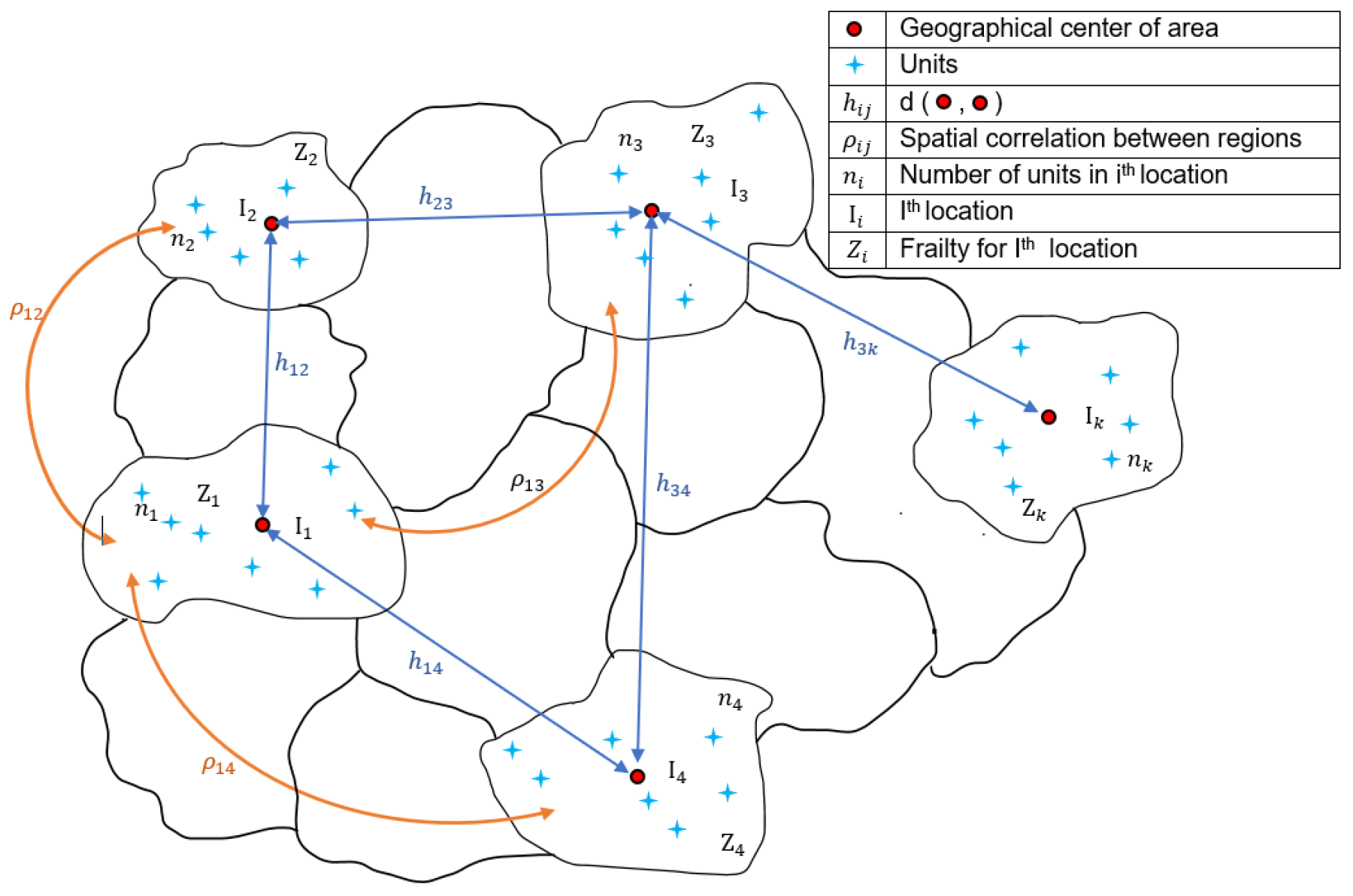
This manuscript is concerned with the development of models for estimating the regression parameters with clustered right censored data that account for spatial patterns between various locations. This is important in the sense that if the spatial impact leads to drastic consequences, local authorities could take necessary preventive actions to reduce damage. It is, therefore, of considerable importance to develop models for estimating the distribution function of time to event while accounting for spatial correlation. We consider multiple units per location in order to reflect the real life situation, and leukemia data will be used for illustration, since it fits more closely with our setting, with a pictorial representation given in Figure 1.
In the above pictorial representation, we show that all units are assumed to be located at the geographical center. Ref. [2] modeled spatial association via a mean random frailty per region, wherein individual frailty Z i within a region j with mean frailty μ j was assumed to follow a gamma distribution, with parameters depending on μ j . The vector ( μ 1 , , μ k ) is assumed to follow a multivariate normal distribution whose variance–covariance matrix is a function of the distance between regions. In this manuscript, we incorporate spatial association in the failure times via a probit transformation, leading to a multivariate Gaussian random field with the spatial correlation matrix being a function of the distance between locations. The two modeling approaches are applied to the same data, and it is shown that embedding the spatial correlation within the failure time results in improvement. Ref. [2] did not provide large sample properties; we did so on all parameters involved in our models for the purpose of making inference and performing further investigations tailored to a specific area.
Though some work has been performed to incorporate spatial correlation in modeling, very few of the works model many units per geostatistical location while accounting for spatial patterns. The aim of this manuscript is to develop statistical models for spatially correlated right censored data for multiple units per location, where regression parameters have a region and/or area level interpretation, and in which spatial correlation is properly incorporated by transforming the original failure times.
The manuscript proceeds as follows. In Section 2, we develop the stochastic process machinery for this type of data and motivate our model choices. Section 3 deals with some preliminary results that will set the stage for the estimation procedures in Section 4. In Section 4, we propose our weighted estimating score processes and show that they are asymptotically unbiased. Section 5 is on the existence of solutions and the infill asymptotic results of the estimators. Section 6 presents the results of our numerical studies, which indicate good approximation to the true parameters, and an illustrative application with the leukemia dataset. The manuscript then concludes with a summary and future directions.

2. Spatially Correlated Right Censored Data and Models

The first critical step in the modeling is to identify a suitable spatial dependence model between locations. As noted earlier, we will focus on a geostatistical formulation that relies on the fitting of covariance and cross-covariance structures for Gaussian random fields for mathematical and computational convenience. This approach also facilitates incorporation of the spatial correlation parameters in the modeling via the covariation process between two locations resulting from the martingale modeling.
To facilitate reading of the manuscript, the following notation on locations and number of units per location will be adopted throughout. We have a total of k locations, with each being described by its longitude and latitude in a two-dimensional coordinate with I i = ( l i 1 , l i 2 ) , which represents the location. If no confusion arises, we will just write location i. The locations will be denoted by i and j, so that i , j { 1 , , k } : = L . Each location i has n i units. Units are denoted by the letters r or s. For instance, in location i, we have r = 1 , , n i so that r { 1 , , n i } : = L i . Likewise, s { 1 , , n j } = L j . For convenience, we may sometimes adopt the compact notation ( i , r ) L × L i , similarly for ( j , s ) .

2.1. Pairwise Right Censored Data

Consider k geographical locations described by two-dimensional coordinates { I i = ( l i 1 , l i 2 ) ; i = 1 , , k } where l i 1 and l i 2 denote longitude and latitude of the ith geographical location, respectively. The I i s represent the geographical centers. Let n i be the number of subjects in the ith geographical location. Each unit is observed until failure or censoring, whichever occurs first. At time t, for the r th ( r = 1 , 2 , , n i ) unit in the i th ( i = 1 , 2 , , k ) geographical location, we record failure or censoring time by W i ( r ) and C i ( r ) , respectively, and these are assumed independent. Let δ i ( r ) = I ( W i ( r ) C i ( r ) ) , T i ( r ) = W i ( r ) C i ( r ) be the usual notation with right censored data. The variable δ i ( r ) indicates that either censoring or failure has occurred for unit r in location i. For ( i , r ) L × L i , a p-dimensional vector x i ( r ) ( t ) of possibly time varying covariates is recorded at time t. Location i is assumed to be spatially correlated with j, i j , and the spatial correlation between the two is denoted by ρ i j : = ρ ( l i l j ) , where l i l j is the Euclidean distance between l i and l j . The total observable entities per location at time t are, therefore,
O ( I i ) = r = 1 n i O ( r ) ( I i ) = r = 1 n i { x i ( r ) ( t ) , T i ( r ) , δ i ( r ) } .
In the present setting of spatially correlated events, the random observables in (1) will be taken pairwise for the purpose of accounting for the spatial correlation ρ i j . Consequently, the spatially correlated right censored data on L , on which estimation is conducted, is given by
O = O ( I i ) , O ( I j ) ; ρ i j ; i j ; ( i , j ) { 1 , , k } 2 = L × L .

2.2. Stochastic Process Modeling

With a view towards the multivariate Gaussian random field (MGRF), we introduce the stochastic processes needed in the following. For ( i , r ) L × L i , define the counting and at-risk process by N i ( r ) ( t ) = δ i ( r ) I ( T i ( r ) t ) and Y i ( r ) ( t ) = I ( T i ( r ) t ) , respectively. Note that N i ( r ) ( t ) indicates if an event has occurred by time t, whereas Y i ( r ) ( t ) indicates if unit ( i , r ) is at risk at time t. One may modify Y i ( r ) ( · ) to allow left truncation or other general at-risk processes. We further assume that the study ends at a time τ so that the interval [ 0 , τ ] = T is our observation window. The entire history at time t at all geostatistical locations is contained in the σ -field F t = i = 1 k r = 1 n i F i , t ( r ) with
F i , t ( r ) = σ N i ( r ) ( t ) , Y i ( r ) ( t ) , t T .
To proceed with our modeling, we assume that the instantaneous hazard function is different from location to location. If λ i ( t ) is the instantaneous failure rate in ( t , t + d t ) for all units in location i, from stochastic integration theory, the compensator process of N i ( r ) ( t ) is A i ( r ) ( t ) given by A i ( r ) ( t ) = 0 t Y i ( r ) ( u ) λ i ( u ) d u . Hence, for each ( i , r ) , the process
M i ( r ) ( t ) = N i ( r ) ( t ) 0 t Y i ( r ) ( u ) λ i ( r ) ( u ) d u : t T
is a zero-mean square-integrable martingale with respect to the filtration F i , t ( r ) . In this manuscript, we postulate the Cox model with a different baseline per location, but the same regression parameter, β , for all locations. The model is given by
λ i ( r ) ( t ) = λ 0 i ( t ) exp ( β x i ( r ) ( t ) ) ,
where a denotes the transpose of the vector a , and β is a p-dimensional vector of regression parameters. The baseline hazard per location is λ 0 i ( t ) , and { λ 0 i ( t ) : i = 1 , , k } is the set of unspecified baseline hazard functions to be estimated.
Remark 1. 
Our choice of same β coefficient for all locations is motivated by the fact that we are modeling the same event for all units in all locations. However, the baseline hazard is chosen to be different among the locations, see also [16,17]. The case of competing failures can also be considered, cf. [18].

2.3. Multivariate Gaussian Random Fields

Gaussian Random Fields (GRFs) and their multivariate counterpart, MGRFs, play an important role in spatial modeling, especially in geostatistics. Estimation of parameters are facilitated if the models proposed can lead to the construction of MGRF using the resulting martingale processes. With a view towards the MGRF construction, for ( i , r ) L × L i , let x i ( r ) : = x i ( r ) ( t ) if ambiguity does not arise, Λ ( t | x i ( r ) ) is the cumulative hazard function, and F ¯ i ( r ) ( t | x i ( r ) ) = exp Λ ( t | x i ( r ) ) is the survival function. Then, F ¯ i ( r ) ( T i ( r ) | x i ( r ) ) follows a uniform distribution on ( 0 , 1 ) , and Λ i ( r ) ( T i ( r ) | x i ( r ) ) follows a unit exponential distribution EXP ( 1 ) . If Φ ( · ) is the cumulative distribution function of the standard normal distribution, the probit transformation of a variable U in ( 0 , 1 ) is Φ 1 ( U ) . Hence,
T ˜ i ( r ) : = Φ 1 1 e Λ 0 i ( T i ( r ) ) exp ( β x i ( r ) )
is the probit transformation of the failure time T i ( r ) , which follows a standard normal distribution of N ( 0 , 1 ) . If we assume that, for each location i, its vector of failure times
T ˜ i = ( T ˜ i ( 1 ) , T ˜ i ( 2 ) , , T ˜ i ( n i ) )
forms a Gaussian random field, then a MGRF can be constructed with T ˜ , given by
T ˜ = T ˜ 1 , T ˜ 2 , , T ˜ k ( n 1 , , n k ) ,
by imposing a spatial structure induced by a ( i = 1 k n i ) × ( i = 1 k n i ) spatial correlation matrix Ξ with block matrices J n i × n i = ( 1 ) n i × n i , i = 1 , , k as diagonal elements, and the off diagonal elements ( n i , n j ) I { i j } depend on the spatial correlation ρ i j between two locations.

2.4. Spatial Correlation Model

As indicated earlier, the critical part in identifying significant risk factors that trigger event occurrences is to identify the best spatial correlation function. Ref. [2] proposed a multivariate gamma frailty model incorporating spatial dependence between locations, as was performed in [5]. Ref. [8] extended the work of [19] by generalizing their Multivariate Conditional Autoregressive Models. A pairwise joint distribution that depends on the distance between locations has been investigated by [10]. Copula models, on the other hand, have been proposed by [20,21]. We seek a spatial correlation that is a function of distance between spatial locations, so-called isotropic spatial covariance functions. They have received a great deal of attention recently, specifically the Matérn family [22,23,24], given by
C ( h ) = σ 2 M ( h ; ν , a ) = σ 2 2 1 ν Γ ( ν ) a h ν K ν a h ,
where σ 2 is the marginal variance or sill, which is the variance if h = l i l j = 0 . ν > 0 is a smoothing parameter that controls the differentiability of a Gaussian process with this covariance; and a > 0 is a range parameter that measures the correlation decay as the separation between two locations increases. K ν ( · ) is the modified Bessel function of the second kind, and Γ ( · ) is the gamma function. When ν = 0.5 and + , we recover the exponential and Gaussian covariance given by
C ( h ) = σ 2 exp ( a h ) ,
C ( h ) = σ 2 exp ( a 2 h 2 ) ,
respectively. More details on sill and range can be found in Section 3 of [25] or Section 1 of [24]. The Matérn family turns out to be a good choice because of its flexibility in modeling various types of spatial correlation structure in many fields, and possesses a good interpretability of the parameters. The importance of this family is also highlighted in [26], page 14. Note that in (3), if i = j , h = 0 , we obtain the marginal variance, which corresponds to the case of no spatial correlation.
In what follows, we assume that the spatial correlation function depends on the q-dimensional parameter δ = ( δ 1 , , δ q ) each describing various elements of the family. A Matérn-type family for spatial correlation on the transformed failure times is assumed, translating into δ = ( σ 2 , r a n g e , s m o t h n e s s ) , which is q = 3 . The transformation leads to a MGRF where the marginal failure times follow the postulated Cox model with a population level interpretation for the regression parameter β , and facilitates estimation of the spatial as well as regression parameters.

3. Estimation-Preliminary

The parameters arose from two models: the spatial correlation and the Cox models. The Cox models have unknown infinite dimensional baseline parameters λ 0 i ( t ) , i = 1 , , k that belong to a class C of hazards on + . The regression coefficient β is in p , whereas the q-dimensional Matérn spatial correlation parameter δ is in q . Though, in the case of the Matérn family, q = 3 , we develop the theory for an unknown q. So, the model parameter of main interest is
θ = [ ( λ 01 ( t ) , , λ 0 k ( t ) ) ; ( β 1 , , β p ) ; ( δ 1 , , δ q ) ] Θ ,
where Θ C k × p × + q . The observable O in (2) will be used for making an inference on θ .
Remark 2. 
Our models have ( k + p + q ) unknowns, which raises the question of identifiability. Let p θ ( · ) be the probability model on O . The issue of identifiability will not arise; that is, the Kullback–Leibler information will be positive for θ θ 0 under the assumptions that, under p θ ( · ) : (i) no two regions have the same longitude and latitude; (ii) for every region i, r = 1 n i Y i ( r ) ( t ) > 0 , that is, at least one failure occurs per region; (iii) for every i, n i 2 ; and (iv) for A G i = σ r = 1 n i Y i ( r ) ( t ) , t T , and B G j (likewise defined), P ( A B ) > 0 . The last assumption ensures estimation of the spatial correlation parameter, hence a uniquely defined spatial correlation function.

3.1. The Aalen–Breslow Estimator of λ 0 i ( t ) and Its Properties

Following the notation in Section 2.3, and as indicated earlier, for each ( i , r ) ,
M i ( r ) ( t ) = N i ( r ) ( t ) 0 t Y i ( r ) ( u ) λ i ( r ) ( u ) d u : t T
is a zero-mean martingale with respect to the filtration F i , t ( r ) . It then follows, via method of moments, that an Aalen–Breslow estimator for Λ 0 i ( · ) = 0 · λ 0 i ( u ) d u , for i L is given by
Λ ^ 0 i ( t ) = 0 t r = 1 n i d N i ( r ) ( u ) r = 1 n i Y i ( r ) ( u ) exp β x i ( r ) ( u ) ,
with the k dimensional vector of baseline hazard being Λ ^ 0 ( t ) = Λ ^ 01 ( t ) , , Λ ^ 0 k ( t ) . Observe that Λ ^ 0 ( t ) is not yet an estimator, because it still depends on the unknown regression parameter β = ( β 1 , , β p ) . The expression in (6) will later be substituted for λ 0 i ( t ) to estimate β and to obtain the in-probability limits of the score matrix.
In order to facilitate understanding of the asymptotic properties of the parameters in our models, it is important to go through some properties of λ ^ 0 i ( t ) = d Λ ^ 0 ( t ) . The consistency of λ ^ 0 i ( t ) can be shown using results in [27].
Remark 3. 
An important result worth pointing out is the convergence under the infill asymptotic of the random field W ^ ( t ) given by
W ^ ( t ) = n Λ ^ 01 ( t ) Λ 01 ( t ) , , Λ ^ 0 k ( t ) Λ 0 k ( t )
to the multivariate Gaussian random field W ( t ) = ( W 1 ( t ) , , W k ( t ) ) on the space of continuous functions D k [ 0 , τ ] , and the k-fold continuous functions space, equipped with the metric d ( f , g ) = max i { 1 , , k } { f i ( t ) g i ( t ) } . Such a result can be used for making simultaneous inferences on Λ 0 i ( t ) at some fixed time points and constructing confidence bands for all the baseline or a subset of them, depending on interest, or testing equality of the baseline hazards at two different locations i and j. The latter and former could be important for epidemiologists and authorities, since the results can be used to assess severity of a certain disease or pandemic at various times of the calendar year or having an idea about which locations among the ones under investigation have higher failure rates.

3.2. Joint Modeling

For a pair of units, ( r , s ) ( L i , L j ) and t [ 0 , τ ] , we define, as before, their counting, at-risk, and compensator processes by
[ N i ( r ) ( t ) , Y i ( r ) ( t ) , A i ( r ) ( t ) ] and [ N j ( s ) ( t ) , Y j ( s ) ( t ) , A j ( s ) ( t ) ] ,
respectively. Then, { M i ( r ) ( t ) : t [ 0 , τ ] } and { M j ( s ) ( t ) : t [ 0 , τ ] } are each a zero-mean martingale with respect to the filtration F i , t ( r ) and F j , t ( s ) , respectively. With a view toward joint modeling, for ( t 1 , t 2 ) [ 0 , τ ] 2 , we introduce the joint counting process N i j ( r , s ) ( · , · ) by N i j ( r , s ) ( t 1 , t 2 ) = I { T i ( r ) t 1 , T j ( s ) t 2 } . The covariance function cov ( M i ( r ) ( t 1 ) , M j ( s ) ( t 2 ) ) is defined by
E ( M i ( r ) ( t 1 ) M j ( s ) ( t 2 ) | T i ( r ) > t 1 , T j ( s ) > t 2 ) = A i , j ( r , s ) ( t 1 , t 2 ) = M i ( r ) ( t 1 ) , M j ( s ) ( t 2 ) .
Using stochastic integration theory, we have
E M i ( r ) ( t 1 ) M j ( s ) ( t 2 ) 0 t 1 0 t 2 Y i ( r ) ( u 1 ) Y j ( s ) ( u 2 ) A i , j ( r , s ) d u 1 d u 2 = 0 .
The spatial correlation between the two locations implies that the covariance function depends on the spatial parameter δ via the spatial correlation ρ i j by virtue of the transformation leading to the construction of the MGRF. Let G ( · , · ; ρ i j ) be the bivariate survival function of the transformed failure times T ˜ i and T ˜ j . Then, the original bivariate survivor function F ¯ i j ( r , s ) ( t 1 , t 2 ; ρ i j ) for ( r , s ) ( L i , L j ) is given by
F ¯ i j ( r , s ) ( t 1 , t 2 ; ρ i j ) = P T i ( r ) > t 1 , T j ( s ) > t 2 ; ρ i j = G Φ 1 ( F i ( r ) ) ( t 1 ) , Φ 1 ( F j ( s ) ( t 2 ) ) ; ρ i j ,
with F i ( r ) ( t 1 ) and F j ( s ) ( t 2 ) being the marginal distribution functions of T i ( r ) and T j ( s ) respectively. Following [28], A i j ( r , s ) ( t 1 , t 2 ) is given by
A i j ( r , s ) ( d t 1 , d t 2 ; ρ i j ) = A 0 [ Λ i ( r ) ( t 1 ) , Λ j ( s ) ( t 2 ) ; ρ i j ] Λ i ( r ) ( d t 1 ) Λ j ( s ) ( d t 2 ) ,
with the baseline joint compensator A 0 [ · , · ; ρ i j ] given by
A 0 ( t 1 , t 2 ; ρ i j ) = 2 t 1 t 2 F ¯ i j ( r , s ) ( t 1 , t 2 ; ρ i j ) + F ¯ i j ( r , s ) ( t 1 , t 2 ; ρ i j ) + t 1 F ¯ i j ( r , s ) ( t 1 , t 2 ; ρ i j ) + t 2 F ¯ i j ( r , s ) ( t 1 , t 2 ; ρ i j ) .
Remark 4. 
The covariance function A i j ( r , s ) ( d t 1 , d t 2 ; ρ i j ) in conjunction with Λ 0 i ( d t 1 ) and Λ 0 j ( d t 2 ) determines the joint distribution of T i and T j , given the covariates x i ( r ) and x j ( s ) . The original bivariate survivor function of T i and T j given in (7) can be taken to be of the Clayton family (cf. [29]) or the Frank family model (cf. [30]). For the Clayton model, for instance, the joint survivor function takes the form
F ¯ ( t i , t j ; ρ i j ) = e t i ρ i j + e t j ρ i j 1 1 ρ i j .

4. Estimation

4.1. Weighted Estimating Functions

Estimation of parameters with spatially correlated random censorship data poses challenges because of: (i) the high dimension of the parameter θ = ( β , δ ; Λ 0 ) , and (ii) the full likelihood that L( θ | Data ) is intractable. Since it is quite difficult to apply direct maximum likelihood method in the spirit of [31], we adopt the pairwise likelihood approach as an alternative. The main reference is [32]. See also [33] for an overview of composite likelihood applications in various fields. Ref. [34] also discusses issues and strategies for the selection of composite likelihood.
The idea is to form pairwise likelihoods, a product of likelihoods for data in two spatial locations that can be the basis of an unbiased estimating function, and then be used for parameter estimation. It is a special case of a more general class of pseudo likelihoods called composite likelihoods, which allows for the addition of likelihoods in a situation where the components do not represent independent replicates. The technique has good theoretical properties, and behaves well in many applications concerning spatial statistics [35,36,37,38,39]. Moreover, it is robust to model misspecification, is computationally advantageous when dealing with data that has a complex structure, and the estimated parameter is the same as in the complete model [34]. In the present setting, for estimating β , and as will be seen later, the covariation of the vector M ( t ) = ( M 1 ( t ) , , M k ( t ) ) depends on the spatial correlation parameter δ and the unequal number of units per geographical site. The spatial dependency between locations may be severe or moderate. As indicated in [40], there may be a loss in efficiency of the estimator of β when accounting for spatial correlation, especially when it is severe. With the aim of increasing efficiency, we follow the idea of [40] by proposing generalized estimating equations that include weights in the estimating functions. The weights are chosen in general to balance out severe versus moderate spatial dependence.
With a view toward estimating β , which accounts for pairwise spatial correlation between two locations ( i , j ) L 2 , we introduce more notation in the following. If a = ( a 1 , a 2 ) is a 1 × 2 row vector and its transpose denoted by a is a 2 × 1 column vector, then for ( r , s ) ( L i , L j ) , define H i j ( r , s ) ( t ) = ( H i ( r ) ( t ) , H j ( s ) ( t ) ) , M i j ( r , s ) ( t ) = ( M i ( r ) ( t ) , M j ( s ) ( t ) ) . The vector H i j ( r , s ) ( t ) is a vector of predictable processes that arises from the martingale modeling and the Doob–Meyer decomposition theorem, cf. [41]. We further define a 2 × 2 matrix W i j ( δ ) = ( w i j ( δ ) ) , whose elements are a function of the spatial correlation δ , and the number of units in locations i and j by
W i j ( δ 0 ) = w 11 i j ( δ 0 ) w 12 i j ( δ 0 ) w 21 i j ( δ 0 ) w 22 i j ( δ 0 ) .
Then, given δ 0 , we define the pairwise estimating equation for β between two locations at time t by
U [ i j ] ( t , β | δ 0 ) = r = 1 n i s = 1 n j 0 t H i j ( r , s ) ( u ) W i j ( δ 0 ) M i j ( r , s ) ( u ) d u .
At time t T , the generalized estimating equation for β over all pairs is
U ( t , β | δ 0 ) = i j U [ i j ] ( t , β | δ 0 ) .
The weight matrix given in (8) adapts to dependencies between locations, especially when dependency is strong and censoring within a location is light, and helps improve efficiency of the estimates under such scenarios. Two remarks are worth mentioning here.
Remark 5. 
Replacing W i j ( δ 0 ) by the identity matrix in (10), we obtain the case of no spatial correlation between locations. Observe also that if W i j ( δ 0 ) is replaced by the variance–covariance matrix of ( M 1 ( t ) , M 2 ( t ) , , M k ( t ) ) with M i ( t ) = r = 1 n i M i ( r ) ( t ) , the weights actually depend on the regression coefficient β, as well as the spatial correlation parameter δ since its compensator A ( t ) depends on both. Then, (10) can be re-expressed as a function of β alone by first replacing δ in (9) by δ ^ , a n = i n i -consistent estimator of δ 0 that satisfies n ( δ ^ δ 0 ) = O p ( 1 ) . In that case, (10) will take the form U ( t ; β , δ ^ ) , and the estimated β would still be consistent. For further discussions, cf. [40]. This approach will be adopted in the estimation of β in the next section.
Remark 6. 
An important property of the estimating function (10) is the robustness of the resulting estimator β ^ , even if the spatial correlation is misspecified and remains asymptotically unbiased even under the misspecification.
Examining U [ i j ] ( · , · | δ 0 ) , we see that it can be written as a sum of four terms, each of which is given below.
U 1 i j ( t ) = r = 1 n i 0 t w 11 i j H i ( r ) ( u , β ) M i ( r ) ( d u ) , U 2 i j ( t ) = r = 1 n i s = 1 n j 0 t w 12 i j H j ( s ) ( u , β ) M i ( r ) ( d u ) , U 3 i j ( t ) = r = 1 n i s = 1 n j 0 t w 21 i j H i ( r ) ( u , β ) M j ( s ) ( d u ) , U 4 i j ( t ) = s = 1 n j 0 t w 22 i j H j ( s ) ( u , β ) M j ( s ) ( d u ) .
For the purpose of estimating δ 0 , note that E { M i ( r ) ( t 1 ) M j ( s ) ( t 2 ) A i j ( r , s ) ( d t 1 , d t 2 ; ρ i j ) } = 0 . The goal is to find a weighted function of M i ( r ) ( t 1 ) M j ( s ) ( t 2 ) A i , j ( r , s ) ( d t 1 , d t 2 ; ρ i j ) that can serve as an estimating function for δ 0 with the flavor of score function. Define the ( k × k ) matrix A ( t 1 , t 2 ; ρ ( δ ) ) = A i j ( t 1 , t 2 ; ρ ( δ ) ) i , j = 1 , , k , with ( i , j ) th entry given by
A i j ( t 1 , t 2 ; ρ ( δ ) = r = 1 n i s = 1 n j A i j ( r , s ) ( t 1 , t 2 ; ρ ( δ ) ) .
Let δ l A ( t 1 , t 2 ; ρ ( δ ) ) , l = 1 , , q , be the matrix of elementwise derivatives of A ( t , ρ ( δ ) ) with respect to δ l . Define
Π l = A 1 δ l A A 1 ,
where we use A for A ( t 1 , t 2 ; ρ ( δ ) ) for compactness. Then, for l = 1 , , q , following [42] (p. 483), we can show that E ( M ( t ) ) Π l E ( M ( t ) ) + t r ( Π l A ) = 0 , where t r ( · ) denotes the trace of a matrix. Consequently, we can define a score function for estimating the lth component of δ using two locations by
U δ l i j ( t 1 , t 2 ) = M ( t ) Π l M ( t ) + t r ( Π l A ) : = M ( t ) Π l M ( t ) + t r ( A 1 A δ l ) .
The expression in (12) can be viewed as a score process, and its sum over all pairwise spatial locations ( i , j ) can serve as an estimating function for δ l . So, the estimating function over all pairs of spatial locations for δ is the q × 1 vector U δ ( t 1 , t 2 ; ρ ( δ ) ) = ( U δ l ( t ) , l = 1 , , q ) where U δ i ( s , t ) is given by
U δ l ( t 1 , t 2 ; ρ ( δ ) ) = ( i , j ) , i j U δ l i j ( t 1 , t 2 ; ρ ( δ ) ) .

4.2. Unbiased Estimating Functions

The unbiased estimating functions concept is one of the requirements for showing the existence of consistent solutions to the equations U δ l ( t 1 , t 2 ) = 0 and U [ i j ] ( β ; · , · | δ 0 ) = 0 , respectively. Two conditions need to be satisfied for the existence and consistency of the estimate: (i) the asymptotic unbiasedness of the two estimating functions, and (ii) the existence of in-probability limit of the information matrix. To show (i) for U δ l ( t ) , the concept of mixing coupled with the multivariate Chebyshev inequality is applied in particular. As for U [ i j ] ( β ; · , · | δ 0 ) = 0 , some regularity conditions applied on its derivatives yield the result. Finally, Theorem 2 of [43] will be used to show existence and consistency of β ^ and δ ^ , the sequence of solutions to the aforementioned equations.
In geostatistics, asymptotic properties can be investigated in two different ways: the increasing domain asymptotic or the infill asymptotic. The increasing domain asymptotic is a sampling structure in spatial statistics, where new observations are added at the boundary points of an area, whereas the infill asymptotic consists of a sampling structure where new observations are added in between existing locations. The latter is appropriate when the spatial locations are fixed and in a bounded domain and one is interested in adding new observations to each location. In this manuscript, we will use the infill asymptotic, since the number of locations is fixed at k. Letting min i { n 1 , , n k } satisfies the infill asymptotic criterion. Therefore, in what follows, the statement n = min i n i means infill asymptotic. Readers are refereed to [42] (Section 7.3.1, p. 480) for details.

Regularity Conditions

I.
For i = 1 , , k , Λ 0 i ( t ) < .
II.
For each ( i , r ) L × L i and t T , x i ( r ) ( t ) is uniformly bounded.
III.
For ( i , r ) L × L i and for each i, define S i ( m ) ( β , t ) = r = 1 n i Y i ( r ) ( t ) [ x i ( r ) ( t ) ] m e β x i ( r ) ( t ) . Let E denote expectation operator. There exists B p , a neighborhood of β 0 , and functions s i ( m ) ( β , t ) , such that E ( S i ( m ) ( β , t ) ) = s i ( m ) ( β , t ) , and that, for each i = 1 , , k , m = 0 , 1 , 2 ,
sup ( β , t ) B × [ 0 , τ ] 1 n i S i ( m ) ( β , t ) s i ( m ) ( β , t ) p 0 ,
and the s i ( m ) ( β , t ) are uniformly bounded on [ 0 , τ ] × B with continuous partial derivatives.
IV.
Define
Ω ^ ( θ ) = Ω ( θ ^ ) = 1 n 2 i j i j E V i j ( θ ^ ) V i j ( θ ^ ) .
There exists a positive definite matrix Ω ( θ 0 ) such that
sup t [ 0 , t * ] Ω ^ ( θ ) Ω ( θ 0 ) p 0 .
V.
Weight matrices conditions:
(i)
W ( δ ) W ( δ 0 ) p 0 , where a b = sup i j | a i j b i j | .
(ii)
For · · { 11 , 12 , 21 , 22 } , β w · · i j ( δ ^ ) p β w · · i j ( δ 0 ) and β w · · i j ( δ ) are continuous functions of δ .
VI.
For · · { 11 , 22 } , m = 0 , 1 , n = i = 1 k n i ,
sup ( β , t ) B × [ 0 , τ ] 1 n i j r = 1 n i H i ( r ) ( t ) w · · i j Y i ( r ) ( t ) e β x i ( r ) ( t ) x i ( r ) m ( t ) s ( w · · ( m ) , β ; t ) p 0 .
sup ( β , t ) B × [ 0 , τ ] 1 n i j s = 1 n j r = 1 n i H i ( r ) ( t ) w 12 i j Y j ( s ) ( t ) e β x j ( s ) ( t ) x j ( s ) m ( t ) s ( w 12 ( m ) , β ; t ) p 0 . sup ( β , t ) B × [ 0 , τ ] 1 n i j s = 1 n j r = 1 n i H j ( s ) ( t ) w 21 i j Y i ( r ) ( t ) e β x i ( r ) ( t ) x i ( r ) m ( t ) s ( w 21 ( m ) , β ; t ) p 0 .
VII. (i)
For ( i , j ) L × L , the weight v i j ( δ ) on the compensators are uniformly bounded with continuous partial derivatives with respect to δ .
VIII.
Joint compensator conditions:
(i)
The function A 0 ( t 1 , t 2 ; δ ) exists and has bounded second derivatives in the range of the arguments ( β , δ ) for all ( β , δ ) B × D , where D q . Moreover, A 0 ( t 1 , t 2 ; δ ) is continuously differentiable as a function of ( β , δ ) and the partial derivative A 0 ( d t 1 , t 2 , δ ) : = A 0 100 , A 0 ( t 1 , d t 2 , δ ) : = A 0 010 , A 0 ( t 1 , t 2 , δ ) : = A 0 001 and A 0 ( d t 1 , d t 2 , δ ) : = A 0 110 are bounded on B × D for all values of the arguments.
(ii)
Any linear combination of the joint compensator partial derivatives with respect to any of its arguments converges to a bounded function.
Discussion of the regularity conditions: Conditions I to III are the regular stability conditions imposed on derivatives of the at-risk process that arise in models that involve the Cox hazard functions. They are the expectations and variances of the covariates x i ( r ) ( t ) of ( i , r ) . Condition V(i) is a stability condition of the weight applied to the estimated spatial correlation parameters, whereas V(ii) is a stability condition guaranteeing convergence of the variance–covariance matrix of the joint process, namely the block Σ 11 . Likewise, Condition VI, together with VII, pertains to infill asymptotic stability of the block Σ 21 and Σ 22 , with VII only needed for the latter.
The following theorem pertains to the asymptotic unbiasedness of U ( β , t ) .
Theorem 1. 
Under Conditions I to V, as n , sup t [ 0 , τ ] 1 n | U ( β , t | δ ^ ) | p 0 .
Proof. 
Using the fact that U [ i j ] ( β , t | δ ^ ) is the sum of four terms, by the triangle inequality, we have
| U [ i j ] ( β , t | δ ^ ) | | U 1 i j ( β , t ) | + | U 2 i j ( β , t ) | + | U 3 i j ( β , t ) | + | U 4 i j ( β , t ) | .
It suffices to show that each term in the RHS of (13) converges to zero in probability. Without loss of generality, we only show that U 1 i j ( β , t ) does. Asymptotic negligibility of the remaining terms are obtained in similar manner. We have
1 n U 1 i j ( β , t ) = 1 n i = 1 k r = 1 n i 0 τ H i ( r ) ( t ) i j w 11 i j s ( t , w 11 ( 0 ) ) s i ( 0 ) ( t ) d M i ( r ) ( t ) 1 s i ( 0 ) ( t ) 0 τ 1 n i i H i ( r ) ( t ) Y i ( r ) ( t ) e β 0 x i ( r ) ( t ) w 11 i j s i ( t , w 11 ( 0 ) ) d M i ( r ) ( t ) s ( w 11 ( 0 ) ( t ) ) 0 τ 1 n i = 1 k Y i ( r ) ( t ) e β 0 x i ( r ) ( t ) 1 s i ( 0 ) ( t ) 1 d M i ( r ) ( t ) 1 n ß j H i ( r ) ( t ) Y i ( r ) ( t ) e β 0 x i ( r ) ( t ) w 11 i j s ( t , w 11 ( 0 ) ) · 0 τ 1 n i = 1 k Y i ( r ) ( t ) e β 0 x i ( r ) ( t ) 1 s i ( 0 ) ( t ) 1 d M i ( r ) ( t ) .
Each one of the terms on the right hand side of (14) is o p ( 1 ) when n , per the regularity conditions I to V. Therefore, n 1 U 1 i j ( β , t ) = o p ( 1 ) . Likewise, under conditions I to V, it can be shown that the remaining three terms in n 1 U [ i j ] ( β , t ) are all asymptotically negligible. Hence, sup t [ 0 , τ ] n 1 U [ i j ] ( β , t | δ ^ ) p 0 as n , completing the proof of the asymptotic unbiasedness of n 1 U [ i j ] ( β , t | δ ^ ) . □
For the purpose of showing unbiasedness of the score associated with the spatial correlation parameter, let v i j be the weight between two sites. The weight v i j can be taken to be a function of the spatial correlation ρ i j ( δ ) between locations i and j, and will help increase efficiency of δ ^ . With no loss of generality, it suffices to consider a score process between two locations of the form
U i j ( t 1 , t 2 ; δ ) = v i j [ M i ( t 1 ) M j ( t 2 ) A i j ( t 1 , t 2 ; δ ) ] ,
where M i ( t 1 ) = r = 1 n i M i ( r ) ( t 1 ) , M j ( t 2 ) = s = 1 n j M j ( s ) ( t 2 ) , and A i j ( t 1 , t 2 ; δ ) = r = 1 n i s = 1 n j A i j ( r , s ) ( t 1 , t 2 ; δ ) . The corresponding estimating function for δ over all pairs is given by
U ( t 1 , t 2 ; δ ) = i j U i j ( t 1 , t 2 ; δ ) .
The next theorem is on the asymptotic unbiasedness of U ( t 1 , t 2 ; δ ) .
Theorem 2. 
Under Conditions VI and VIII, as n , we have
U ( t 1 , t 2 ; δ ) = 1 n ( i , j ) , i j U i j ( t 1 , t 2 ; δ ) p 0 .
Proof. 
We use the mixing condition, along with Chebyshev inequality and Condition VII. Let I n ( ι n ) = { i , j / i j ι n } . The set I n ( ι n ) gives the range beyond which the spatial correlation impact is negligible. The cut off point ι n depends on the number of locations. In what follows, A denotes the complement of a set A. For ϵ > 0 , we have, via Chebyshev inequality and Condition VII,
P n 1 ( i , j ) , i j U i j ( t 1 , t 2 ; δ ) > ϵ = P ( i , j ) , i j v i j M i ( t 1 ) M j ( t 2 ) > n ϵ + ( i , j ) , i j v i j A i j ( t 1 , t 2 ) ( i , j ) , i j E ( v i j M i ( t 1 ) M j ( t 2 ) ) ( n ϵ + ( i , j ) , i j v i j A i j ( t 1 , t 2 ) ) 2 ( i , j ) I n ( ι n ) E ( M i ( t 1 ) M j ( t 2 ) ) n 2 ϵ 2 + ( i , j ) I n ( ι n ) E ( M i ( t 1 ) M j ( t 2 ) ) n 2 ϵ 2 .
With a proper choice of mixing function, the last inequality in previous display converges to 0 under the mixing condition VII. □

5. Large Sample Properties

This section is devoted to the large sample properties of our estimators. Let θ = ( β , δ ) , U 1 ( β , t ) = U [ i j ] ( t , β | δ 0 ) and U 2 ( t 1 , t 2 ; δ ) = U i j ( t 1 , t 2 ; δ ) . Consider the vector of score processes V ( t ) = ( U 1 ( β , t ) , U 2 ( t 1 , t 2 ; δ ) ) , such that
V ( θ ; t , t 1 , t 2 ) = V ( θ ) = 1 n i j U 1 ( β ) U 2 ( δ ) = 1 n i j U [ i j ] ( t , β | δ 0 ) U i j ( t 1 , t 2 ; δ ) : = 1 n i j V i j ( θ ; t , t 1 , t 2 ) .
The in-probability limit of the variance–covariance matrix of V ( θ ; t , t 1 , t 2 ) is given by
Σ n = 1 n i j θ V i j ( θ ; t , t 1 , t 2 ) = β U 1 ( β , t ) δ U 1 ( β , t ) β U 2 ( δ , t ) δ U 2 ( δ ; t 1 , t 2 ) p Σ = Σ 11 Σ 12 Σ 21 Σ 22 .
The next theorem is on the existence and consistency of the solution to V ( θ ) = 0 .
Theorem 3. 
(a) 
There exists a sequence of solutions β ^ n and δ ^ n to the sequence of estimating equations U 1 ( β , t ) = 0 and U 2 ( t 1 , t 2 ; δ ) = 0 .
(b) 
Under Conditions I to VIII, and the infill asymptotic, β ^ n p β 0 and δ ^ n p δ 0 .
Before proving the theorem, a discussion on λ ^ 0 i ( t ) , i = 1 , , k is warranted, since its consistency is required for the in-probability limit of the score variance. A method of moment estimator of λ ^ 0 i ( t ) is given by
λ ^ 0 i ( t ) = r = 1 n i d N i ( r ) ( t ) S i ( 0 ) ( β , t ) ,
and is a jump process, and will possibly loses efficiency for large n. However, any loss of efficiency using it for the limit is minor as compared to using a more complicated smoothed estimator obtained via kernel and proposed in [27], given by
λ ^ 0 i K ( t ) = 1 h n 0 t K t u h n d Λ ^ 0 i ( u ) ,
where K ( · ) is some kernel function, and h n is a sequence of positive constants. Although λ ^ 0 i K ( t ) is smoother, both are, however, consistent for λ 0 i ( t ) ; that is, sup t [ 0 , τ ] | λ ^ 0 i ( t ) λ 0 i ( t ) | p 0 . We will proceed with the version λ ^ 0 i ( t ) .
Proof. 
We apply the inverse function theorem of [43]. Three conditions need to be satisfied: (i) the asymptotic unbiasedness of the estimating functions, (ii) the existence and continuity of the partial derivatives matrix, and (iii) the negative definiteness of the matrix of partial derivatives at the true parameter value θ 0 . Condition (i) has been already shown in Theorems 2 and 3. It remains to show (ii) and (iii). Consider U 1 i j ( t ) given by
U 1 i j ( t ) = 1 n i j r = 1 n i 0 τ w 11 i j H i ( r ) ( u , β ) M i ( r ) ( d u ) .
Since λ 0 i ( t ) is unknown, we substitute it by its consistent Breslow estimator. So, the version we work with is U ^ 1 i j ( t ) , given by
U ^ 1 i j ( t ) = 1 n i j r = 1 n i 0 t w 11 i j H i ( r ) ( u , β ) · d N i ( r ) ( u ) Y i ( r ) ( u ) e β x i ( r ) ( u ) r = 1 n i d N i ( r ) ( u ) S i ( 0 ) ( β , u ) · r = 1 n i d N i ( r ) ( u ) S i ( 0 ) ( β , u ) .
The gradient of U ^ 1 i j ( t ) with respect to β is
β U ^ 1 i j ( β , τ ) = 1 n i j r = 1 n i 0 τ β H i ( r ) ( u , β ) · w 11 i j d N i ( r ) ( u ) Y i ( r ) ( u ) e β x i ( r ) ( u ) λ ^ 0 i ( u ) d u + 1 n i j r = 1 n i 0 τ H i ( r ) ( u , β ) w 11 i j S i ( 1 ) ( β , u ) S i ( 0 ) ( β , u ) λ ^ 0 i ( u ) d u Y i ( r ) x i ( r ) ( u ) e β x i ( r ) ( u ) λ ^ 0 i ( u ) d u + Y i ( r ) ( u ) e β x i ( r ) ( u ) S i ( 1 ) ( β , u ) S i ( 0 ) ( β , u ) λ ^ 0 i ( u ) d u p o p ( 1 ) 0 τ s u ; β , w 11 ( 0 ) s i ( 1 ) ( β , u ) s i ( 0 ) ( β , u ) s u ; β , w 11 ( 1 ) λ 0 i ( u ) d u .
Likewise, substituting the Breslow estimator in U ^ 2 i j ( t ) , the gradient of U ^ 2 i j ( t ) is
β U ^ 2 i j ( β , τ ) = 1 n i j s = 1 n j r = 1 n i 0 τ β H j ( s ) ( u , β ) w 12 i j d N i ( r ) ( u ) Y i ( r ) ( u ) e β x i ( r ) ( u ) λ ^ 0 i ( u ) d u + 1 n i j r = 1 n i 0 τ H j ( s ) ( u , β ) w 12 i j + Y i ( r ) ( u ) e β x i ( r ) ( u ) S i ( 1 ) ( β , u ) S i ( 0 ) ( β , u ) λ ^ 0 i ( u ) d u Y i ( r ) ( u ) x i ( r ) ( u ) e β x i ( r ) ( u ) λ ^ 0 i ( u ) d u + Y i ( r ) ( u ) e β x i ( r ) ( u ) S i ( 1 ) ( β , u ) S i ( 0 ) ( β , u ) λ ^ 0 i ( u ) d u p o p ( 1 ) 0 τ s t ; β , w 12 ( 0 ) s i ( 1 ) ( β , u ) s i ( 0 ) ( β , u ) s u ; β , w 12 ( 1 ) λ 0 i ( u ) d u .
Taking the gradient with respect to β of the remaining two terms in U ^ [ i j ] ( t ) , and taking their limits according to the regularity conditions, we obtain that, at θ 0 , the first block of Σ , namely Σ 11 = σ i j i , j = 1 , , k , with the ( i , j ) t h element given by
σ i j = 0 τ s u ; β , w 11 ( 0 ) s i ( 1 ) ( β , u ) s i ( 0 ) ( β , u ) s u ; β , w 12 ( 0 ) s i ( 1 ) ( β , u ) s i ( 0 ) ( β , u ) s u ; β , w 11 ( 1 ) s u ; β , w 12 ( 1 ) 0 τ s u ; β , w 11 ( 0 ) s i ( 1 ) ( β , u ) s i ( 0 ) ( β , u ) s u ; β , w 12 ( 0 ) s i ( 1 ) ( β , u ) s i ( 0 ) ( β , u ) λ 0 i ( u ) d u 0 τ s u ; β , w 11 ( 0 ) s i ( 1 ) ( β , u ) s i ( 0 ) ( β , u ) s u ; β , w 22 ( 0 ) s j ( 1 ) ( β , u ) s j ( 0 ) ( β , u ) s u ; β , w 22 ( 1 ) s u ; β , w 21 ( 1 ) 0 τ s u ; β , w 11 ( 0 ) s i ( 1 ) ( β , u ) s i ( 0 ) ( β , u ) s u ; β , w 12 ( 0 ) s i ( 1 ) ( β , u ) s i ( 0 ) ( β , u ) λ 0 j ( u ) d u .
Note that σ i j is a p × p matrix. Obviously, Σ 12 = 0 , a matrix of 0. The Σ 22 block is the gradient of U 2 ( δ ; t 1 , t 2 ) with respect to δ . To see how it is derived, let v i j be a 1 × q row vector and δ A i j ( t 1 , t 2 ; δ ) be defined by
v i j = ( v 1 i j , , v q i j ) ; δ A i j ( t 1 , t 2 ; δ ) = δ 1 A i j , , δ q A i j : = δ A i j .
respectively. To make the notation compact, for l = 1 , , q , let
δ l A i j ( t 1 , t 2 ; δ ) = δ l A i j ( ( δ ) ) = δ l A i j ( δ ) : = A δ l i j .
Then, the ( i , j ) t h element of Σ 22 is the q × q matrix given by
Σ 22 i j ( δ ) = v i j δ A i j = v 1 i j A δ 1 i j v 1 i j A δ 2 i j v 1 i j A δ q i j v 2 i j A δ 2 i j v 2 i j A δ 2 i j v 2 i j A δ q i j v q i j A δ 1 i j v q i j A δ 2 i j v q i j A δ q i j .
Recall also that
δ l A i j ( δ ) = r = 1 n i s = 1 n j δ l A i j ( r , s ) ( t 1 , t 2 , ; δ ) .
So that, for example, the ( 1 , 1 ) component of Σ 22 i j is given by
Σ 22 i j ( 1 , 1 ) = v 1 i j A δ 1 i j = v 1 i j r = 1 n i s = 1 n j δ 1 A i j ( r , s ) ( t 1 , t 2 ; δ ) .
The in-probability limit of Σ 22 i j ( 1 , 1 ) is
Σ 22 i j ( 1 , 1 ) = lim n 1 n i j v i j δ 1 A i j ( t 1 , t 2 ; δ ) .
By virtue of the previous derivations, a compact notation for Σ 22 is then
Σ 22 = lim n 1 n i j r = 1 n i s = 1 n j v i j δ A i j ( r , s ) ( t 1 , t 2 ; δ ) .
That limiting matrix is assumed to exist per Condition VII, and is negative definite.
We now deal with the block Σ 21 . It is easy to show that the ( i , j ) th element, i = j = 1 , , k , of the gradient of U 2 ( t 1 , t 2 ; δ ) , with respect to β , is Σ 21 i j
Σ 21 i j = 0 τ v i j r = 1 n i H i ( r ) ( u , β ) S i ( 1 ) ( β , u ) S i ( 0 ) ( β , u ) · r = 1 n i Y i ( r ) ( u ) e β x i ( r ) ( u ) s = 1 n j M j ( s ) ( x j ( s ) ( u ) ) + r = 1 n i s = 1 n j A i j ( r , s ) ( d u 1 , u 2 ; ρ ( δ ) ) λ ^ 0 i ( u ) d u + 0 τ v i j s = 1 n j H j ( s ) ( u , β ) S j ( 1 ) ( β , u ) S j ( 0 ) ( β , u ) · s = 1 n j Y j ( s ) ( u ) e β x j ( s ) ( u ) r = 1 n i M i ( r ) ( x i ( r ) ( u ) ) + r = 1 n i s = 1 n j A i j ( r , s ) ( u 1 , d u 2 ; ρ ( δ ) ) λ ^ 0 j ( u ) d u .
Note that Σ 21 i j is a p × p matrix, and the in-probability limit, assuming we can interchange the integration operation and limit, is given by
E ( Σ 21 i j ) = lim n 1 n ( i , j ) , i j Σ 21 i j .
Hence, the partial derivative matrix converges to a matrix Σ , which is negative definite at the true parameter value ( β 0 , δ 0 ) . It then follows from the inverse function theorem of [43] that there exists a unique sequence ( β ^ , δ ^ ) , such that V ^ ( t ; β ^ , δ ^ ) = 0 and ( β ^ , δ ^ ) p ( β 0 , δ 0 ) as n . □
The next theorem is on the asymptotic normality of ( β ^ n , δ ^ n ) when properly standardized.
Theorem 4. 
Under regularity Conditions I and VIII,
n { ( β n ^ , δ n ^ ) ( β 0 , δ 0 ) } d N p + q ( 0 p + q , Φ ) ,
where Φ is a ( p + q ) × ( p + q ) matrix given by Φ = Σ 1 Ω Σ 1 .
Proof. 
We apply the central limit theorem for random field given in Remark (3), page 112, of [44]. Taylor expansion of V ( t , θ ) at θ = θ 0 yields
n ( θ n ^ θ 0 ) = θ V ( t , θ ) θ = θ * 1 n V ( t , θ 0 ) ,
where θ * is between θ n ^ and θ 0 , and θ * p β 0 under the infill asymptotic domain setting. Furthermore, note that
θ V ( t , θ ) θ = θ * p Σ
as n . The Ω matrix in Φ is the variance of the score vector which, under Conditions V and VI, is assumed to exist, and converges to a positive definite matrix. The expression of Φ is obtained by applying the result of multivariate central limit theorem. Finally, the theorem follows upon applying Remark (3), page 112, of [44]. □

6. Numerical Assessment and Application

6.1. Numerical Assessment

In this subsection, we present and discuss the results of our simulation studies. This begins with the selection of the different regions that will be used. The package raster on Geographic Data Analysis and Modeling contains the geographical coordinates of many countries. We used the United States as the country.
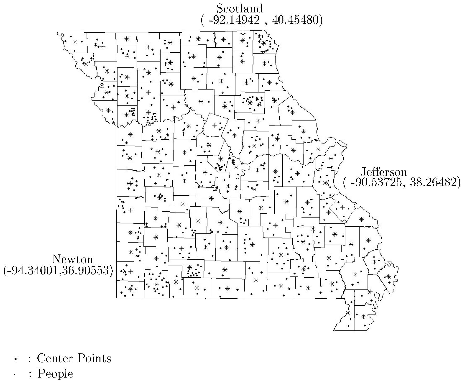
- Regions: The raster package (v.3.6-26) in R contains the data on the geographical coordinates of well-defined subdivisions in many countries. We used the package to obtain the coordinates for states, counties etc. for the United States. Depending on the country, this package also allows users to select location data with several levels of depth. For the United States, we can specify either Level 1 for statewise locations or Level 2 for the countywise locations. We use Level 1 data from raster for the simulations. The geographical centers of the 48 contiguous states, excluding Hawaii and Alaska, are our I i , i = 1 , , 48 . The other alternative is to choose a state and randomly select counties within the selected state. In Figure 2, we provide the example of the state of Missouri with the coordinates for a couple of the counties. For example, the longitude and latitude of the center of Newton county in the state of Missouri is ( 94.34 , 36.91 ) .
- Simulation design: We select a random sample of { n i : i = 1 , . . , 48 } people from each state, where n i is proportional to the state population from the latest census available in R, while making sure that n = i = 1 48 n i { 500 , 5000 , 50,000 } . We consider two covariates x = ( x 1 , x 2 ) , where x 1 follows the binomial distribution with parameters n = n i and p = 0.5 , and x 2 N ( 0 , 0.5 ) , resulting in a mixture of categorical and quantitative covariates. The spatial correlation parameter was set at δ = ( δ 1 , δ 2 ) = ( range , sill ) = ( 0.5 , 1.5 ) . The regression coefficient vector in the Cox model is β = ( β 1 , β 2 ) = ( 1 , 2 ) . As for the proportion of censored observation, we allow from less censoring to severe censoring in order to assess its impact on the spatial correlation. The proportion of censored units was taken to be in { 5 % , 10 % , 20 % , 25 % } , allowing for mild to severe censoring. For the baseline hazard, we use the Weibull hazard given by λ 0 ( t ) = θ 1 θ 2 ( θ 1 t ) θ 2 1 . We set θ 1 = 1 , since it is the scale parameter and is irrelevant in our simulation. However, the shape parameter θ 2 was taken in { 0.8 , 1.5 } to allow for increasing failure over time for θ 2 = 2 and decreasing for θ 2 = 0.8 .
- Event times generation: Under the Cox model with Weibull baseline hazard, we generate failure times via the probit transformation using the following steps:
(i)
If Φ ( · ) denotes the probit transformation, then solving for the Cox’s model, we obtain for ( i , r ) L × L i
Λ 0 i ( T i ( r ) ) = ln 1 Φ ( T ˜ i ( r ) ) exp [ β x i ( r ) ( t ) ] .
Solving for T i ( r ) , we obtain
T i ( r ) = Λ 0 i 1 ln 1 Φ ( T ˜ i ( r ) ) exp ( β x i ( r ) ( t ) ) ,
where Λ 0 i 1 ( · ) is the inverse of the Weibull cumulative hazard given by Λ 0 1 ( t ) = t 1 θ 2 .
(ii)
For ( i , r ) L × L i , the T i ( r ) s are generated using the expression
T i ( r ) = ln 1 Φ ( T ˜ i ( r ) ) exp ( β x i ( r ) ( t ) ) 1 θ 1 ,
where Φ ( T ˜ i ( r ) ) U ( 0 , 1 ) .
- Simulated data: For the purpose of estimating parameters, the study considers two spatial correlation models, namely the exponential and Gaussian model, as given in (4) and (5), and the powered spatial correlation function. For all models, 500 simulation replications were performed with each parameter specification and sample size combination. The results are given in Table 1, Table 2 and Table 3. CP stands for censoring percentage.
Comments on the simulation results: The results of the simulation study indicate that the estimators of the spatial correlation δ , as well as regression coefficients β , perform well. One thing to note here is that as the percentage of censoring increases, the biases of the β increase, regardless of the sample size, whereas the biases of the δ remain very steady close to each other. This makes sense, since the spatial correlation parameters is the correlation between two areas, so it is not affected by large samples. However, the bias of β will increase because higher censoring translates into less failure times. There is no significant difference in the results between the exponential and Gaussian spatial correlation models. The reason why this is so is both have exponential components, so the impact of the large sample will be minor. However, the standard deviations of the estimates of δ remain, without any noticeable pattern with the increasing sample size.

6.2. Illustrative Application

The foregoing procedures are applied to the leukemia survival data which was also analyzed in [2]. The data contains 1043 cases of Acute Myeloid Leukemia (AML) which were recorded between 1982 and 1998 at 24 administrative districts. It contains the time T i ( r ) for each unit ( i , r ) L × L i , and the censoring indicator δ i ( r ) . There were 16% of censored observations. Four covariates were available; that is, x = ( a g e , g e n d e r , w b c , t p i ) , where wbc stands for white blood cell count and tpi for Townsend score. The Townsend score is a qualitative value in [ 7 , 10 ] describing quality of life in a given area. High values indicate less affluent areas. We investigate the factors affecting survival while accounting for spatial correlation. 
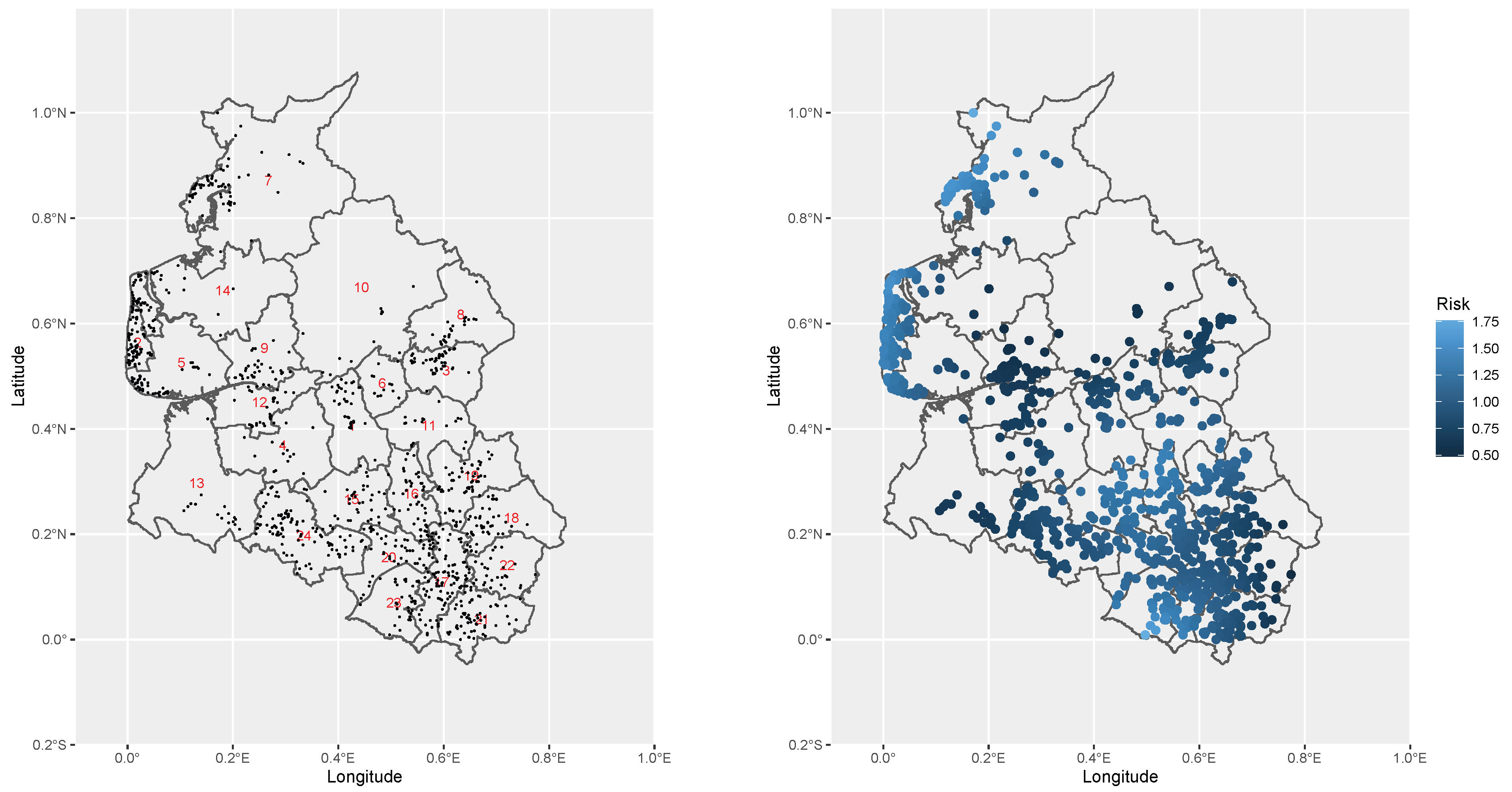
Figure 3 shows residential locations of the AML cases during the observation window. Ref. [2] investigated whether the survival distribution in AML in adults is homogeneous across the region after allowing for known risk factors. In their manuscript, they employ a multivariate frailty that incorporates the effects of covariates, individual heterogeneity, and spatial traits. Our approach and theirs are different. Whereas we both use the Cox model as the instantaneous failure rate, their approach in studying spatial variation is performed via the use of conditional frailty, where the conditioning random variable for all 24 districts is the vector of mean frailty μ = ( μ 1 , , μ 24 ) . Specifically, if Z r is the frailty for unit r in location I j , and μ j the mean frailty of all individuals in that location, they postulate that
Z r | μ j Γ ( ξ 1 , ( ξ μ j ) 1 ) ,
with a N ( 1 , Ξ ) distribution on μ j , where Ξ measures the spatial variation between districts. Whereas they use a conditional frailty model with a variance–covariance matrix that is a function of the distance between regions, we embed the spatial correlation in the transformed failure times, giving us a multivariate Gaussian random field with variance–covariance that is a function of the distance between regions via the Matérn spatial correlation function.
Before applying our methods, we run a set of initial data analysis. 
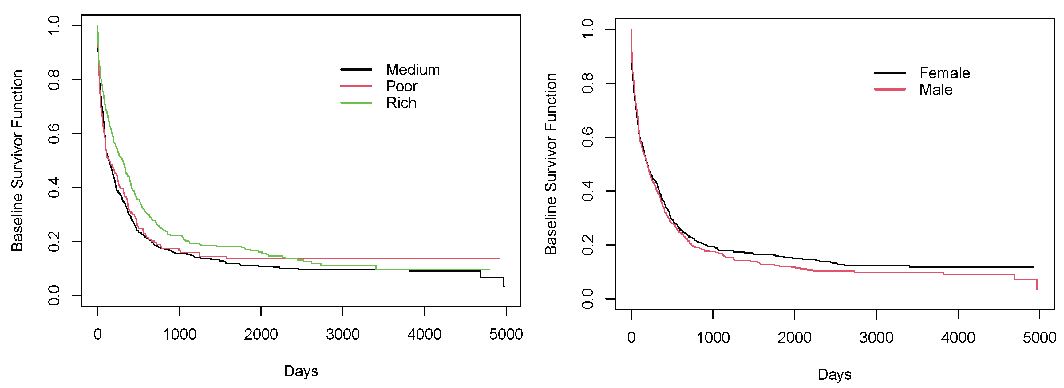
Figure 3 shows the Kaplan–Meier plots by gender. We can clearly observe that survival curve for the female group lies above that of male group. This concurs with the summary statistics in Table 4. The variable tpi represents the Townsend score. The higher values for tpi indicates less affluent areas. We have grouped all individuals in the study into three categories based on tpi. If the tpi of a person is lower than 1.5 , he or she is categorized into the Rich group. Likewise, if the tpi of a person falls between 1.5 and 4.5 , the person is grouped into the Medium category. Lastly, if a person’s tpi is greater than 4.5 , that person is categorized into the Poor group. Figure 4 presents the survival curves according to these three areas. From near day 100 to 5000, the survival curve of the Medium group always lies below the survival curves of the other two groups. Moreover, when we compare the survival curves of the Poor and Rich groups, from day 0 to near day 2400, the survival curve for the Rich group is always above the Poor group. But, interestingly, we can see that from near day 2400 to 5000, the survival curve for the Poor group is above that of the Rich group.
We apply our methods to analyze the leukemia data. Factors that may increase the risk of acute myeloid leukemia include age, gender, prior cancer treatment, environmental factors, blood disorder, and genetic disorder, to name a few. We only consider available covariates in the data, and assumed that age at onset of acute myeloid leukemia (AML) on adults follows the Cox model. We used the Matérn model to account for the spatial dependence between pair of districts. The hazard function for an rth unit in district i is given by
λ i ( r ) ( t ) = λ 0 i ( t ) exp [ β a g e age + β s e x sex + β w p c wpc ]
We estimated the regression coefficients and the spatial correlation parameters using the estimating functions in Section 5. We also calculated the associated standard deviations and confidence intervals. The results are presented in Table 5. We have also presented the results of Henderson’s approach in Table 6. The results in both tables show in both models that all regression coefficients are significant in both approaches expect that sex is not significant under the Henderson approach. So, the covariates age and wpc increase the risk of aml. In our approach, sex also increases the risk of aml, and the results concur with our preliminary analysis of the data. The estimated value of the range, which is 1.2418 , indicates that the impact of environment vanishes when two units are separated by at least 1.2418 units of distance. The log pseudo marginal likelihoods (LPMLs) for each model are also given. Despite the fact that our model has more parameters, it has a better LPML. However, this needs to be taken with cautious and deep investigation, such as taking into account that each unit personal geographical location would be needed to arrive at the best model in this situation. Conclusions between the two competing approaches follow.

7. Concluding Remarks

We have considered the situation where many units clustered in different geographical areas described by their longitude and latitude are monitored for the occurrence of some event. We have developed a methodology using a combination of modern survival analysis and geostatistics formulation. The parameters of our models are estimated using unbiased estimating functions, and their large sample properties were also examined using infill asymptotic approach that one encounters with spatial data. The methodology can be easily generalized to the case of recurrent events. Another generalization is to consider the geographical coordinate of each unit within a given geographical area. One can then consider both within and between areas spatial correlation. It will be of interest to develop models that account for correlation between event time via frailty when the event is allowed to recur. Another possible future direction is another model for modeling connection between failure covariates and failure times, such as the accelerated failure time model. However, other estimating approaches, such as rank-based, would need to be applied to the transformed event times. The Cox model used in the modeling may not fit the real data. Additional goodness-of-fit tests should be conducted before adopting the Cox model. The same is true for the spatial correlation function. This can be checked using the periodogram; likewise for the spatial correlation. The regularity conditions on which the asymptotic properties are obtained may also not be satisfied in practice, leading to limitations in the application of the composite likelihood. For future studies, hypotheses testing on hazard functions that account for spatial correlations need to be developed. Likewise, techniques for assessing the fit of the spatial correlation function also need to be investigated, so that practitioners will have the necessary tools at their disposal for applications to real-life data. The weak convergence result in Remark 3 also needs to be proven, so that confidence bands can be developed to identify severe areas, especially if the models are used for biomedical applications such as pandemics.

Author Contributions

Methodology, F.Z.S.A. and A.A.; Formal analysis, S.D.N. All authors have read and agreed to the published version of the manuscript.

Funding

This research received no external funding.

Data Availability Statement

No new data were created or analyzed in this study. Data sharing is not applicable to this article.

Conflicts of Interest

The authors declare no conflicts of interest.

References

  1. Goldstein, H. Multilevel Statistcal Models; Edward Arnold: New York, NY, USA, 1995. [Google Scholar]
  2. Henderson, R.; Shimakura, S.; Gorst, D. Modeling spatial variation in leukemia survival data. J. Am. Stat. Assoc. 2002, 97, 965–972. [Google Scholar] [CrossRef]
  3. Gorst, D. North West Leukaemia Register; Technical Report; Leukaemia Register: London, UK, 1995. [Google Scholar]
  4. Li, Y.; Ryan, L. Modeling spatial survival data using semiparametric frailty models. Biometrics 2002, 58, 287–297. [Google Scholar] [CrossRef] [PubMed]
  5. Banerjee, S.; Wall, M.; Carlin, B. Frailty modeling for spatially correlated survival data, with application to infant mortality in Minnesota. Biostatistics 2003, 4, 123–142. [Google Scholar] [CrossRef] [PubMed]
  6. Banerjee, S.; Dey, D.K. Semiparametric proportional odds models for spatially correlated survival data. Lifetime Data Anal. 2005, 11, 175–191. [Google Scholar] [CrossRef]
  7. Li, Y.; Lin, X. Semiparametric normal transformation models for spatially correlated survival data. J. Am. Stat. Assoc. 2006, 101, 591–603. [Google Scholar] [CrossRef]
  8. Diva, U.; Banerjee, S.; Dey, D.K. Modelling spatially correlated survival data for individuals with multiple cancers. Stat. Model. 2007, 7, 191–213. [Google Scholar] [CrossRef]
  9. Diva, U.; Dey, D.K.; Banerjee, S. Parametric models for spatially correlated survival data for individuals with multiple cancers. Stat. Med. 2008, 27, 2127–2144. [Google Scholar] [CrossRef]
  10. Paik, J.; Ying, Z. A composite likelihood approach for spatially correlated survival data. Comput. Stat. Data Anal. 2012, 56, 209–216. [Google Scholar] [CrossRef] [PubMed]
  11. Pan, C.; Cai, B.; Wang, L.; Lin, X. Bayesian semiparametric model for spatially correlated interval-censored survival data. Comput. Stat. Data Anal. 2014, 74, 198–208. [Google Scholar] [CrossRef]
  12. Hunt, F.Y. Genetic and Spatial Variation in Some Selection-Migration Models. Ph.D. Thesis, New York University, New York, NY, USA, 1978. [Google Scholar]
  13. Bronnenberg, B.J. Spatial models in marketing research and practice. Appl. Stoch. Models Bus. Ind. 2005, 21, 335–343. [Google Scholar] [CrossRef]
  14. Engen, S. Stochastic growth and extinction in a spatial geometric Brownian population model with migration and correlated noise. Math. Biosci. 2007, 209, 240–255. [Google Scholar] [CrossRef]
  15. Matheron, G. Traité de Gostatistique Appliquée; Statistics for Biology and Health, Editions Technip: Paris, France, 1962; pp. xiv+333. [Google Scholar]
  16. Spiekerman, C.F.; Lin, D.Y. Marginal regression models for multivariate failure time data. J. Am. Stat. Assoc. 1998, 93, 1164–1175. [Google Scholar] [CrossRef]
  17. Lin, D.Y. Cox Regression Analysis of Multivariate Failure Time Data: The Marginal Approach. Stat. Med. 1994, 13, 2233–2247. [Google Scholar] [CrossRef]
  18. Wei, L.J.; Lin, D.Y.; Weissfeld, L. Regression analysis of multivariate incomplete failure time data by modeling marginal distributions. J. Am. Stat. Assoc. 1989, 84, 1065–1073. [Google Scholar] [CrossRef]
  19. Banerjee, S.; Carlin, B. Semi-parametric spatiotemporal analysis. Environmetrics 2003, 14, 523–535. [Google Scholar] [CrossRef]
  20. Lawless, J.F.; Yilmaz, Y.E. Semiparametric estimation in copula models for bivariate sequential survival times. Biom. J. 2011, 53, 779–796. [Google Scholar] [CrossRef] [PubMed]
  21. Yilmaz, Y.E.; Lawless, J.F. Likelihood ratio procedures and tests of fit in parametric and semiparametric copula models with censored data. Lifetime Data Anal. 2011, 17, 386–408. [Google Scholar] [CrossRef]
  22. Matérn, B. Spatial Variation, 2nd ed.; Lecture Notes in Statistics; With a Swedish Summary; Springer: Berlin, Germany, 1986; Volume 36, p. 151. [Google Scholar] [CrossRef]
  23. Guttorp, P.; Gneiting, T. Studies in the history of probability and statistics. XLIX. On the Matérn correlation family. Biometrika 2006, 93, 989–995. [Google Scholar] [CrossRef]
  24. Gneiting, T.; Kleiber, W.; Schlather, M. Matérn cross-covariance functions for multivariate random fields. J. Am. Stat. Assoc. 2010, 105, 1167–1177. [Google Scholar] [CrossRef]
  25. Handcock, M.S.; Stein, M.L. A Bayesian Analysis of Kriging. Technometrics 1993, 35, 403–410. [Google Scholar] [CrossRef]
  26. Stein, M.L. Interpolation of Spatial Data; Springer Series in Statistics; Some theory for Kriging; Springer: New York, NY, USA, 1999; pp. xviii+247. [Google Scholar] [CrossRef]
  27. Ramlau-Hansen, H. Smoothing counting process intensities by means of kernel functions. Ann. Stat. 1983, 11, 453–466. [Google Scholar] [CrossRef]
  28. Prentice, R.L.; Cai, J. Covariance and survivor function estimation using censored multivariate failure time data. Biometrika 1992, 79, 495–512. [Google Scholar] [CrossRef]
  29. Clayton, D.G. A model for association in bivariate life tables and its application in epidemiological studies of familial tendency in chronic disease incidence. Biometrika 1978, 65, 141–151. [Google Scholar] [CrossRef]
  30. Genest, C. Frank’s family of bivariate distributions. Biometrika 1987, 74, 549–555. [Google Scholar] [CrossRef]
  31. Jacod, J. Un théorème de représentation pour les martingales discontinues. Z. Wahrscheinlichkeitstheorie Verw. Geb. 1976, 34, 225–244. [Google Scholar] [CrossRef]
  32. Lindsay, B.G. Composite likelihood methods. In Comtemporary Mathematics; American Mathematical Society: Providence, RI, USA, 1988; Volume 80, pp. 221–239. [Google Scholar] [CrossRef]
  33. Varin, C.; Reid, N.; Firth, D. An overview of composite likelihood methods. Stat. Sin. 2011, 21, 5–42. [Google Scholar]
  34. Lindsay, B.G.; Yi, G.Y.; Sun, J. Issues and strategies in the selection of composite likelihoods. Stat. Sin. 2011, 21, 71–105. [Google Scholar]
  35. Hjort, N.L.; Omre, H. Topics in spatial statistics. Scand. J. Stat. 1994, 21, 289–357, With discussion and a reply by the authors. [Google Scholar]
  36. Heagerty, P.J.; Lele, S.R. A composite likelihood approach to binary spatial data. J. Am. Stat. Assoc. 1998, 93, 1099–1111. [Google Scholar] [CrossRef]
  37. Lele, S.; Taper, M.L. A composite likelihood approach to (co)variance components estimation. J. Stat. Plan. Inference 2002, 103, 117–135, C. R. Rao 80th birthday felicitation volume, Part I. [Google Scholar] [CrossRef]
  38. Varin, C.; Vidoni, P. A note on composite likelihood inference and model selection. Biometrika 2005, 92, 519–528. [Google Scholar] [CrossRef]
  39. Varin, C.; Hø st, G.; Skare, O.i. Pairwise likelihood inference in spatial generalized linear mixed models. Comput. Stat. Data Anal. 2005, 49, 1173–1191. [Google Scholar] [CrossRef]
  40. Liang, K.Y.; Zeger, S.L. Longitudinal data analysis using generalized linear models. Biometrika 1986, 73, 13–22. [Google Scholar] [CrossRef]
  41. Andersen, P.K.; Gill, R.D. Cox’s regression model for counting processes: A large sample study. Ann. Stat. 1982, 10, 1100–1120. [Google Scholar] [CrossRef]
  42. Cressie, N.A.C. Statistics for Spatial Data; Wiley Series in Probability and Mathematical Statistics: Applied Probability and Statistics; John Wiley & Sons, Inc.: New York, NY, USA, 1993; pp. xxii+900, Revised reprint of the 1991 edition, A Wiley-Interscience Publication. [Google Scholar] [CrossRef]
  43. Foutz, R.V. On the consistency of locally asymptotically most stringent tests. Can. J. Stat. 1976, 4, 211–219. [Google Scholar] [CrossRef]
  44. Guyon, X. Random Fields on a Network; Probability and Its Applications (New York); Springer: New York, NY, USA, 1995; pp. xii+255, Modeling, statistics, and applications, Translated from the 1992 French original by Carenne Ludeña. [Google Scholar]
Figure 1. Pictorial representation of the setting.
Mathematics 12 01521 g001
Figure 2. Missouri county map.
Mathematics 12 01521 g002
Figure 3. Leukemia data with the 24 districts (left panel) and leukemia data with the 24 districts, units, and risk (right panel).
Mathematics 12 01521 g003
Figure 4. Survival curve of areas categories (left panel) and survival curve of gender (right panel).
Mathematics 12 01521 g004
Table 1. Numerical results for the for Matérn exponential correlation function when α 2 = 1.5 .
CPn β ¯ 1 σ ^ β 1 β ¯ 2 σ ^ β 2 δ ¯ 1 σ ^ δ 1 δ ¯ 2 σ ^ δ 2
5%94,2900.96300.04041.92050.08020.47610.05531.47060.0757
157,1500.97900.04001.94950.07910.46990.04321.47340.0461
314,3000.96550.03411.92930.06480.48760.05521.51000.0782
10%94,2900.95590.04061.90640.08190.52980.05521.48690.0699
157,1500.97250.04051.93540.08020.47100.05501.47010.0545
314,3000.95880.03431.91480.06570.50890.06141.51260.0538
20%94,2900.93970.04101.87430.08370.53090.05071.51660.0253
157,1500.95640.04151.90400.08220.49680.05611.45390.0429
314,3000.94250.03561.88310.06800.48340.05951.45570.0563
25%94,2900.93060.04201.85600.08520.53230.06251.44180.0684
157,1500.94740.04191.88690.08320.48920.06091.50270.0422
314,3000.93360.03621.86630.06940.47970.04101.51950.0527
Table 2. Numerical results for the for Matérn exponential correlation function when α 2 = 0.8 .
CPn β ¯ 1 σ ^ β 1 β ¯ 2 σ ^ β 2 δ ¯ 1 σ ^ δ 1 δ ¯ 2 σ ^ δ 2
5%94,2900.96280.03951.92020.07850.48980.05881.48970.0279
157,1500.97920.03931.95000.07770.51570.04291.45840.0301
314,3000.96560.03331.92940.06330.49770.04151.52480.0604
10%94,2900.95570.03971.90590.08040.52680.06251.47050.0543
157,1500.97280.03971.93590.07880.51270.05641.51050.0435
314,3000.95880.03361.91480.06420.49560.06071.51430.0471
20%94,2900.93950.04011.87390.08220.51140.04391.47180.0634
157,1500.95670.04081.90440.08080.47730.04581.49310.0694
314,3000.94240.03491.88310.06660.48710.05191.48780.0562
25%94,2900.93050.04111.85560.08380.50930.04941.53450.0582
157,1500.94770.04131.88740.08180.48810.05181.47660.0346
314,3000.93360.03551.86610.06800.47470.05801.46280.0440
Table 3. Numerical results for the powered correlation function when α 2 = 0.8 .
CPn β ¯ 1 σ ^ β 1 β ¯ 2 σ ^ β 2 δ ¯ 1 σ ^ δ 1 δ ¯ 2 σ ^ δ 2
5%94,2900.9760.0551.9510.1070.5060.0711.5230.057
157,1500.9700.0521.9350.1020.4940.0551.4970.021
314,3000.9600.0531.9140.1040.5030.0591.5070.062
10%94,2900.9470.0361.9110.0670.5070.0481.4990.058
157,1500.9880.0451.9290.0910.4790.0581.4930.043
314,3000.9450.0381.8830.0760.5070.0581.4900.075
20%94,2900.9530.0431.8840.0880.4670.0491.5420.067
157,1500.9540.0511.9050.1020.5080.0361.5060.040
314,3000.9340.0471.8630.0910.5080.0521.4810.053
25%94,2900.9430.0491.8720.0970.5020.0651.5040.059
157,1500.9430.0591.8810.1220.5020.0431.5020.077
314,3000.9560.0441.9070.0900.4870.0491.5000.063
Table 4. Summary statistics of leukemia data by gender.
FemaleMale
Survival time in daysMin1.01.0
Q137.045.5
Q2182.0186.0
Mean581.5489.0
Q3574.8490.5
Max4922.04977.0
AgeMin14.0014.0
Q148.0050.0
Q265.0065.0
Mean60.9860.5
Q375.0074.0
Max92.0092.0
wbcMin0.000.00
Q11.801.70
Q27.358.10
Mean40.4236.94
Q336.6041.10
Max500.00500.00
Table 5. Summary of means and standard deviations of regression parameters and spatial parameters for leukemia data using our models. L P M L = 5991.082 .
MeanMedianStd.Dev. 95 % CI-Low 95 % CI-Upp
age30.65 × 10 3 27.95 × 10 3 3.70 × 10 3 27.95 × 10 3 34.69 × 10 3
sex70.40 × 10 3 70.61 × 10 3 0.30 × 10 3 70.07 × 10 3 70.61 × 10 3
wbc3.00 × 10 3 3.03 × 10 3 0.04 × 10 3 2.95 × 10 3 3.03 × 10 3
tpi34.30 × 10 3 33.77 × 10 3 0.72 × 10 3 33.77 × 10 3 35.09 × 10 3
sill891.25 × 10 3 913.18 × 10 3 48.35 × 10 3 815.88 × 10 3 913.18 × 10 3
range1241.79 × 10 3 1201.53 × 10 3 90.02 × 10 3 1201.53 × 10 3 1382.70 × 10 3
Table 6. Summary of means and standard deviations of regression parameters and spatial parameters for leukemia data using Henderson’s model. L P M L = 5925.385 .
MeanMedianStd.Dev. 95 % CI-Low 95 % CI-Upp
age51.95 × 10 3 52.00 × 10 3 3.35 × 10 3 45.07 × 10 3 58.46 × 10 3
sex108.04 × 10 3 105.01 × 10 3 108.38 × 10 3 −101.16 × 10 3 325.87 × 10 3
wbc5.94 × 10 3 5.94 × 10 3 0.79 × 10 3 4.39 × 10 3 7.53 × 10 3
tpi61.37 × 10 3 61.24 × 10 3 15.46 × 10 3 33.07 × 10 3 93.25 × 10 3
fv64.22 × 10 3 40.42 × 10 3 80.68 × 10 3 1.01 × 10 3 252.93 × 10 3
Disclaimer/Publisher’s Note: The statements, opinions and data contained in all publications are solely those of the individual author(s) and contributor(s) and not of MDPI and/or the editor(s). MDPI and/or the editor(s) disclaim responsibility for any injury to people or property resulting from any ideas, methods, instructions or products referred to in the content.

