Abstract
In rough set theory, a construct is an attribute subset with the same ability to discern objects belonging to different classes as the whole set of attributes, while maintaining the similarity between objects belonging to the same class. Although algorithms for reducts computation can be adapted to compute constructs, practical problems exist where these algorithms cannot compute all constructs within a reasonable time frame. Therefore, this paper introduces an algorithm for computing all constructs of a decision system. The results of experiments with various decision systems (both artificial and real-world) suggest that our algorithm is, in most cases, faster than the state-of-the-art algorithms when the simplified binary discernibility–similarity matrix has a density of less than 0.29.
MSC:
68T37; 68T30; 68Q25; 68T10
1. Introduction
In rough set theory (RST) [1], constructs [2], like reducts [3], are subsets of attributes that allow discerning objects belonging to different classes to at least the same extent as the complete set of attributes, but unlike reducts, constructs also maintain similarity between objects belonging to the same class. Thus, although constructs are commonly larger than reducts, they are a better option for building a reduced representation of a decision system preserving as much knowledge as possible. Constructs can be used to build rule-based classifiers [4], as feature selectors [5], in problems of reduction of the representation space of the objects [6], among others.
The most challenging problem related to constructs involves computing all constructs of a decision system, which is an NP-hard problem (reducible to the Boolean satisfiability problem (SAT) in polynomial time). On the other hand, computing constructs has been little explored; only a few studies have proposed methods to compute constructs using algorithms designed for reducts computation [7,8]. The study presented in [7] is focused on computing constructs using algorithms that compute reducts working on the discernibility function. In contrast, the study presented in [8] focuses on computing constructs using algorithms for reducts computation that operate on the binary discernibility matrix.
Although both works introduce methods that allow computing all constructs using algorithms designed to compute reducts, it is worth mentioning that, for reducts computation, in most datasets, it is better to operate with the binary discernibility matrix rather than the discernibility function, since by considering specific properties of Boolean operations and their bitwise implementations, faster executions of the algorithms can be achieved [9,10].
Because of the above-mentioned, an algorithm for computing all constructs in a dataset, based on the method described in [8], is introduced in this paper. The algorithm introduced in this work for computing all constructs uses the concepts of gap elimination and attribute contribution (denoted as CC-GEAC), which is also used in the most successful algorithms for reducts computation reported in the literature [10,11,12]. The CC-GEAC algorithm introduces a pruning strategy that allows for the a priori discarding of some attribute subsets. This pruning strategy avoids unnecessary evaluations conducted during the computation of constructs with the most successful algorithms for reducts computation: fast-CT_EXT [11], fast-BR [12], and GCreduct [10] following the method described in [8], as will be demonstrated later. Based on our experiments, it is observed that CC-GEAC, in most cases, evaluates fewer candidates than the three algorithms above when they calculate all the constructs following [8].
In summary, the contributions of this paper are as follows:
A new algorithm based on gap elimination and attribute contribution is proposed for computing all constructs in a binary matrix calculated from a dataset, as described in [8].
This algorithm includes a pruning strategy that allows for the a priori discarding of more attribute subsets than other pruning strategies (also based on gap elimination and attribute contribution) used in state-of-the-art algorithms.
The rest of this document is organized as follows: Section 2 reviews the related works. In Section 3, basic concepts are presented. The CC-GEAC algorithm is introduced in Section 4. The experiments and results are shown in Section 5, and finally, in Section 6, our conclusions and some directions for future work are provided.
2. Related Works
Constructs computation has been little explored, as mentioned earlier. This section reviews the works reported in the literature on this issue.
In [13], the concept of a construct is introduced, and the relation between reducts and constructs is studied. In this work, Susmaga mentioned that constructs could be computed using a proper modification of an algorithm for reducts computation. This work adapted the fast reducts generating algorithm (FRGA) proposed in [14] to compute constructs.
In [7], a new method for computing constructs of a DS is introduced. The method consists of processing different parts of the object’s pairwise comparison matrix (PCM) [15] to generate inter-class reducts, intra-class reducts, and constructs. This method has two phases: in the first phase, empty, repeated, and non-minimal elements (attribute subsets) with respect to inclusion are eliminated from the PCM; from this phase, the sorted absorbed pairwise comparison list is obtained. In the second phase, the SAPCL is provided as the input to an algorithm for reducts computation. The result of the second phase constitutes the output of the algorithm (i.e., the set of reducts/constructs). The particular type of output is determined by the type of PCM supplied as input to the first phase of the algorithm [7]. This method allows computing constructs using algorithms for reducts computation as long as these algorithms work on the discernibility function.
In [8], the relationship between constructs, reducts, and irreducible testors is studied, showing how algorithms for computing irreducible testors, designed into the logical combinatorial pattern recognition approach [16], can be used to compute constructs. Although the authors did not propose a new algorithm, this work increases the set of available algorithms for reducts computation that can be used for computing constructs, since the authors provide a way to compute constructs by defining a new binary matrix, where algorithms to compute reducts and irreducible testors can be used for computing constructs. This new matrix is constructed by comparing all pairs of objects in different ways, depending on whether or not they belong to the same class, unlike the binary discernibility matrix that only considers pairs of objects belonging to different classes. In this way, when two objects from different classes are compared, if an attribute distinguishes these objects, a 1 in the corresponding matrix entry is put. It means that this attribute should be taken into account when a construct is built. Otherwise, when the objects under comparison belong to the same class, if an attribute does not distinguish these objects, a 1 is placed in the corresponding matrix entry. This is because the attribute contributes to preserving the similarity between the objects. This means that this attribute should be taken into account when a construct is built. As shown in [17], reducts and irreducible testors (IT) are closely related concepts, and under certain conditions, they coincide. Therefore, constructs can be computed by methods for computing reducts and irreducible testors by using this new binary matrix.
Even though either method, [7] or [8], could be used to compute constructs, the problem of finding all constructs has been little explored. This justifies the search for more efficient algorithms to compute constructs.
3. Basic Concepts
In RST, the data in a supervised classification problem are represented by a decision system (DS). Formally, a DS can be represented by a pair , where:
- represents a finite non-empty set of objects called universe;
- denotes a finite non-empty set of attributes, such that and ; being the set of condition attributes and d the decision attribute.
For every attribute , there is an information function , where is a finite non-empty set of values for the attribute a, and denotes the value corresponding to the object in the attribute a.
A DS is commonly represented as a matrix, in which columns are associated with attributes, rows to objects, and cells to attribute values of objects. A DS is considered consistent if any combination of values from the entire set of condition attributes defines the value of the decision attribute; otherwise, it is considered inconsistent.
To express the fact that a set of attributes cannot discern objects in a DS, the indiscernibility relation [1], is defined for a non-empty set of attributes as follows:
If a pair of objects belongs to , the objects cannot be differentiated from each other given the attributes of the subset .
Before formally defining the construct concept, it is important to introduce the definitions of discernibility relation and similarity relation [13].
The discernibility relation, denoted as , is defined as follows:
This means that if a pair of objects belongs to , then x and y differ from each other by at least one attribute from the set .
On the other hand, the similarity relation, denoted as , is defined for a set of attributes as follows:
If a pair of objects belongs to , then these two objects are similar in at least one attribute from the set .
A construct (introduced by R. Susmaga in [13]) is an attribute subset of condition attributes that maintains the discernibility between pairs of objects belonging to different classes with the same capability as the whole set of condition attributes, while simultaneously ensuring similarity between objects belonging to the same class. The definition of a construct can be stated as follows:
Condition (1) means that a construct discerns objects belonging to different classes. Moreover, according to condition (2), a construct guarantees similarity between objects belonging to the same class. Condition (3) ensures minimality regarding inclusion, which means that removing any attribute from will make Conditions (1) or (2) invalid.
The set of all attributes contained in all constructs is called a kernel. It is important to highlight that the kernel could be empty.
Since the algorithm proposed in this article works on a binary matrix similar to the binary discernibility matrix, first, we will define the binary discernibility matrix, which is used by the most successful algorithms for computing all reducts.
The binary discernibility matrix (BDM), proposed by Felix and Ushio [18], is a binary representation of the discernibility matrix proposed by Skowron and Rauszer [19].
Definition 2.
Given a , the , is a matrix , where each row i results from comparing two objects (u and w) that do not belong to the same class , i.e.,:
where denotes the value of the attribute in the object u, denotes the value of the decision attribute in the object u, and is computed as follows:
4. Proposed Algorithm
Our algorithm (CC-GEAC) goes through the subsets of attributes in a particular order, checking for each one if it is a construct. This verification is conducted on a binary matrix built from a decision system. This binary matrix was first introduced in [8]; it contains all pairs of object comparisons (attribute per attribute). In this work, we will refer to it as the binary discernibility–similarity matrix (BDSM), and it is defined by:
where , , and are as in Definition 2.
The BDSM often contains redundant information, so it can be simplified. Next, some definitions used to simplify the BDSM will be introduced.
Definition 3.
Let be a BDSM, i and f be two rows in , and i is a sub-row of f if and only if:
- (i)
- ;
- (ii)
- .
Example 1.
Suppose and are rows within a specific BDSM, i is a sub-row of f, since f has 1 everywhere i has 1, and there is at least one column, such that f has 1 and i has 0.
Those rows for which there are no sub-rows are called basic rows and are defined as follows:
Definition 4.
Let and f be defined as before. Row f is a basic row of if and only if sub-row .
The matrix formed by the basic rows of the BDSM, without repeating, will be denoted as the simplified binary discernibility–similarity matrix ().
CC-GEAC traverses the search space looking for super-constructs and then checks minimality regarding inclusion (Condition (3) of Definition 1); thus, it is necessary to define the concept of the super-construct in the . Below, some definitions are provided to help define this concept.
Let be an and be an attribute subset. denotes the sub-matrix of , containing only columns corresponding to attributes in .
Definition 5.
Let be an , be an attribute subset, and r be a row of ; r is denoted as a zero-row if it contains only zeros.
Given an , the super-construct definition (Definition 1) can be expressed as follows.
Proposition 1.
Let and as before. is a super-construct in if and only if in there is no zero-row.
Proof.
First, let us consider that is a subset of attributes satisfying Proposition 1 and suppose that is not a super-construct; hence, does not satisfy Conditions (1) or (2) of Definition 1, then objects x and y exist in , (), such that if , then for all a in , which, according to Definition 2, means that in , there is a zero-row, or in another case, if , then for all , one has that , and according to Definition 2, one has a zero-row in . In either case, the hypothesis that satisfies Proposition 1 is contradicted.
Let us assume that, as a hypothesis, is a super-construct in , i.e., satisfies Conditions (1) and (2) of Definition 1. And let us suppose that a zero-row exists in , then according to Definition 2, there are either two objects of the same class () that differ in all attributes of , or there are two objects of different classes () that are indistinguishable in all attributes of , which contradicts the hypothesis; therefore, satisfies the proposition 1. □
Proposition 1, analogous to Conditions (1) and (2) of Definition 1, ensures that a super-construct distinguishes between objects of different classes and guarantees similarity between objects of the same class. Therefore, if an attribute subset does not satisfy Proposition 1, this subset is not a construct.
CC-GEAC generates subsets of attributes following the lexicographic order, like in [20], to traverse the search space. Hereinafter, whenever we refer to a subset of condition attributes, it is considered to be an ordered set of attributes according to this lexicographical order. The ⊕ operator will be used to denote the concatenation of two disjoint ordered subsets of attributes. In this way, and ; note that by concatenating two ordered subsets, the resulting subset maintains the order of the elements in these subsets, and the order in which these subsets are concatenated is relevant. Therefore, concatenation is non-commutative. Moreover, denotes that precedes in the lexicographical order, and denotes that precedes but .
The CC-GEAC algorithm uses the gap concept introduced for the LEX algorithm [20]. The gap of an ordered attribute subset is the rightmost attribute whose succeeding attribute in is not its succeeding attribute in (column in SBDSM); e.g., consider , for , there is no gap; for , the gap is ; finally, for , the gap is .
The pruning property of gap elimination has been used for computing irreducible testors and reducts [10,20]. The same property can be enunciated, adapting it to the and the super-construct concept, as expressed in Proposition 2.
Proposition 2.
Let be an and be a construct, such that and is the last attribute in . If there is a gap in and ; then, there is no construct , such that .
Proof of Proposition 2.
Let , and , then and can be written as and . Let be an ordered attribute subset, such that , so can be written as . Knowing that is a gap (all attributes in are consecutive in ) and is the last attribute in , we can guarantee that and, hence, . From this, cannot be a construct by condition (3) of Definition 1 (minimality condition). □
From Proposition 2, we have the following corollary.
Corollary 1.
Let be as in Proposition 2, and let be a non-super-construct, such that is the last attribute in . If there is a gap in , and ; then, there is no construct , such that .
Using Proposition 2 and Corollary 1, in both cases, all attribute subsets between and can be discarded.
One of the recently proposed pruning strategies is also used in our proposal, which is based on the definition of attribute contribution, which, in our case, is adapted to the as follows:
Definition 6.
Let be as before, be a subset of condition attributes, and be a condition attribute, such that . The attribute contributes to if and only if the number of zero rows in the sub-matrix is less than the number of zero rows in the sub-matrix .
Definition 6 means that an attribute contributes to a given subset, which does not contain it if the new increased subset is capable of distinguishing more objects from different classes or making more objects from the same class appear similar than the original subset.
In CC-GEAC, the columns in are represented as binary words, the length of which is equal to the number of rows in the matrix. The cumulative mask [12] for an attribute , denoted as , is a binary representation of the ith column in the and the cumulative mask for an attribute subset is defined as (∨ denotes the binary OR operator). The number of in is equal to the number of zero rows in for a given . According to Definition 6, contributes to if and only if has more 1’s than . The proposed algorithm generates subsets of attributes in increasing order following the lexicographical order introduced in [20], so the cumulative mask can be computed as . Notice that, from Definition 6, contributes to if and only if since cannot have less 1’s than . From Proposition 1, it can be seen that is a super-construct if and only if .
The exclusion mask, defined for the first time in [21], is relevant to determine whether or not a super-construct is a construct.
Definition 7.
Let and be as before. denotes the exclusion mask of , and it is defined as the binary word that has a 1 in the ith bit if the ith row in has a 1 in only one of the columns corresponding to the attributes in ; the remaining bits of are zeros. Let be an attribute, such that . The exclusion mask of is computed as follows:
where is the cumulative mask, and ¬ is the binary operator for negation.
Example 2.
Let , , and be subsets of attributes of a SBDSM:
| 1 | 0 | 1 | 0 | 1 | 0 | |
| 0 | 1 | 0 | 1 | 1 | 1 | |
| 1 | 1 | 0 | 1 | 0 | 0 | |
| 1 | 0 | 0 | 1 | 1 | 1 | |
| 0 | 0 | 1 | 1 | 1 | 0 | |
| 0 | 1 | 1 | 1 | 0 | 1 | |
| 1 | 0 | 1 | 1 | 0 | 0 |
The corresponding cumulative and exclusion masks are as follows:
The following proposition represents a contribution to the cumulative calculation of the exclusion mask.
Proposition 3.
Let and be as defined in Definition 7. Let . If , such that , then cannot be a subset of any construct, and is said to be exclusionary with .
Proof of Proposition 3.
First, suppose that , such that . Now, suppose that is a subset of a construct; thus, is an essential attribute, which implies that there is a zero-row in the sub-matrix , such that the bit in associated with the row is 1. Thus, by Definition 7, the bit in is associated with the row is 1. So we can conclude that if is a subset of a construct, which is a contradiction ⊥. □
Proposition 3 allows all supersets of to be discarded when is exclusionary with . In what follows, the application of Proposition 3 will be referred to as the exclusion evaluation.
Proposition 4.
Let be a subset of condition attributes and be a condition attribute, such that . is a construct if and only if and is non-exclusionary with .
Proof of Proposition 4.
First, suppose that ; therefore, is a super-construct by Proposition 1. Then, if is non-exclusionary with , all attributes in are essential attributes by Proposition 3, which means that removing an attribute from would invalidate any (or both) of the Conditions (1) or (2) of Definition 1. Thus, we can conclude that is a construct. □
To reduce the search space, Proposition 5 is used to determine a priori if a zero-row prevails after adding any of the remaining attributes to the current attribute subset. This idea was introduced in [22] as a pruning strategy to compute the minimum-length irreducible testor. Similarly, it can be used to prune the search space for computing constructs.
Proposition 5.
Let be an , be a subset of condition attributes, and be a condition attribute, such that . If there is a zero-row r in , such that , then is not contained in any construct.
Proof of Proposition 5.
Since there is a zero-row r in , is not a construct. By hypothesis, if we consider , the row r prevails as a zero-row, even if we add any attribute in . So, we can conclude that will not be a subset of any construct. □
Corollary 2.
Let be an , be a non-super-construct, and be a condition attribute, such that . If there is a zero-row r in , such that , then there is no construct , such that , where .
Consequently, following Proposition 5 and Corollary 2, all attribute subsets between and can be discarded.
Next, we introduce the definition of a zero mask to determine, a priori and in constant time, whether a zero-row will prevail after adding any remaining attributes to the current attribute subset.
Definition 8.
Let be as before; we define the zero mask of a condition attribute , denoted as , to the binary word that has a one in the bit if the row in has a one in any of the (at least one) columns corresponding to the condition attributes , such that , and it is 0 otherwise. The zero mask of is computed as follows:
where refers to the cumulative mask.
By using Definition 8, we can discard some subsets of attributes, thereby pruning the search space. To facilitate this, the following proposition is introduced.
Proposition 6.
Let , , and be as in Proposition 5. If , then is not a subset of any construct.
Proof of Definition 8.
Since , there is a zero-row r in that remains as a zero-row in , even if we add any attribute in . So, we can conclude that is not a subset of any construct. □
CC-GEAC, unlike the algorithms reported in [10,11,12], uses the kernel [7] and the minimum attribute subset [11] together to reduce the number of generated subsets.
Next, the kernel definition is introduced, given a simplified binary discernibility–similarity matrix.
Definition 9.
Let be an and be the set of condition attributes associated with the columns in . The kernel of is defined as:
Given a simplified binary discernibility–similarity matrix (), according to Definition 9, if, in , there exists a row with all zeros except for one column, the attribute corresponding to the column with the value 1 is indispensable for discriminating objects from different classes or maintaining similarity between objects in the same class. Therefore, this attribute must belong to every construct and, consequently, to the kernel. Attributes that meet this condition, and only those, belong to the kernel. It is evident that the kernel is a subset of every construct.
On the other hand, following [11], those attributes in the row with the least amount of 1’s belong to the minimum attribute subset (MSA). Therefore, if the kernel is not empty, MSA has one attribute, which also belongs to the kernel. For this reason, in this paper, the rows with only a “1” are not considered to compute the MSA. Accordingly, given an , the definition of the minimum attribute subset (MSA) used in this paper is as follows:
Definition 10.
Let be the sub-matrix resulting from eliminating the rows with just a 1 in the , be the set of condition attributes, and f be the row with the least number of 1’s in (if there is more than one row, any one of them can be selected). The minimum attribute subset (MSA) is the subset:
In CC-GEAC, the kernel is computed first. Then if the kernel is a construct, it will be the unique construct in the . Otherwise, if the kernel is not a construct, to search for constructs, only those subsets contained in will be taken into account by the algorithm, being:
The attributes in are relabeled, such that the first q attributes belong to the following the order in , and the remaining attributes are attributes in that neither belong to the kernel nor the MSA; the last attributes also follow the order in , e.g., let , , and the , then according to Equation (6) , where , , , , .
CC-GEAC uses Proposition 5 and Corollary 2 to determine if there is a zero-row after adding all the remaining attributes in to the current attribute subset. If there is no zero-row, the attribute contribution condition is verified. If the new attribute contributes, it is checked whether the current candidate (the current attribute subset along with the added attribute) is a super-construct. If the current candidate is a super-construct, then, using Proposition 3, CC-GEAC determines whether the candidate is a construct; if it is a construct, the candidate is saved. At this stage, the algorithm generates the following attribute subset, pruning those subsets that cannot lead to a construct based on Corollary 2 and Corollary 1. The CC-GEAC algorithm continues this process until the first attribute in the current attribute subset no longer belongs to the MSA.
Algorithm 1 shows the pseudo-code of CC-GEAC. The CC-GEAC algorithm operates over the simplified binary discernibility–similarity matrix (SBDSM). First, the is computed. If the kernel is a super-construct, the algorithm ends by returning the kernel as the only construct. Otherwise, the MSA is computed to form set , which will be considered to generate the candidate subsets to evaluate. The current attribute subset is initialized with the first attribute in , and then the cumulative mask is updated. Then, if after adding one of the remaining attributes to the current attribute subset, there is no zero-row (using Proposition 6), the attribute contribution (Definition 6) is evaluated. For those attribute subsets with a contributing attribute (candidates), the super-construct condition (Proposition 1) is evaluated. Proposition 3 is applied to each found super-construct to determine whether it is a construct that will be saved in the result . Candidate evaluation ends at this point, and the next attribute subset in lexicographical order is generated by calling nextSet().
| Algorithm 1: All Constructs Computation |
 |
The procedure for updating the CM of a candidate () appears in Algorithm 2. The CM is stored in an array, indexed by the index in of the last attribute in the current attribute subset (). The last attribute in is determined using , while stores the CM of the kernel.
| Algorithm 2: UpdateCM |
 |
The gap elimination is performed through Algorithm 3. Every consecutive attribute in the current attribute subset, beginning from the last attribute, is removed. In Algorithm 3, the variable q keeps the index in of the last attribute in , while p keeps track of the index of the last attribute in .
| Algorithm 3: RemoveGAP |
 |
Algorithm 4 performs the exclusion evaluation. Firstly, it computes the exclusion mask by applying Equation (5) (see Definition 7). Then by applying Proposition 3, each attribute in the current attribute subset is evaluated for exclusion. Thus, using Proposition 4, it is possible to determine whether or not the current candidate is a construct.
| Algorithm 4: Exclusion |
 |
Algorithm 5 shows the pseudocode for generating the following attribute subset and determining the index in of the next attribute to be processed according to the lexicographic order. First, using Proposition 6, it is determined if there is a zero-row after adding to all of the remaining attributes, for , where i is the index in of the current attribute. If there is no zero-row, if the last attribute in is included in the current candidate, and if the current candidate is not a super-construct (Proposition 2) or a construct (Proposition 4), the gap is removed. Otherwise, the following attribute subset is generated in lexicographical order as follows:
- If the current candidate is a super-construct or the current attribute does not contribute to ; the next attribute in is then considered, which is . Thus, if the current candidate is a super-construct or if does not contribute to , all supersets of are discarded.
- If the current candidate is not a super-construct and contributes to ; then is included in and the next attribute in is set as the current attribute, i.e., .
| Algorithm 5: NextSet |
 |
As described above, the search space is traversed following the lexicographical order, evaluating some attribute subsets and discarding others. First, the kernel and the MSA are computed to reduce the number of generated and evaluated attribute subsets (the kernel is contained in all constructs, and every construct must have at least one attribute from the MSA). The time complexity in the worst case for computing the kernel and the MSA is , where n is the number of columns and m is the number of rows in the SBDSM. On the other hand, the time complexity for updating the cumulative mask, checking for zero rows, and determining if the current attribute subset is a super-construct is in all cases. To check if a super-construct is a construct, firstly, the exclusion mask is computed; after that, the attribute exclusion is evaluated, which is . Generating the following attribute subset, we have , as in the worst-case scenario, all n attributes of the current subset must be analyzed. Since the exclusion evaluation has the highest time complexity in CC-GEAC, the time complexity for evaluating a candidate is . Therefore, since, in the worst case, the number of evaluated candidates has an exponential relation with the number of attributes (n), CC-GEAC has an exponential complexity in terms of the number of attributes. Thus, our algorithm has the same complexity as the algorithms designed to compute reducts or IT that can be used for computing constructs following the process described in [8]. In the next section, some experiments regarding runtimes showing the performance of CC-GEAC are discussed.
5. Experiments and Results
The CC-GEAC algorithm uses the binary discernibility–similarity matrix to compute constructs following the process described in [8]. Hence, to assess our algorithm in Section 5.1, we present a runtime comparison of CC-GEAC against the option of computing constructs following [8] using the fastest algorithms for reducts computation currently available: Fast-CT-EXT [11], FastBR [12], and GCreduct [10], over SBDSMs computed from real-world datasets taken from [23,24,25]. Subsequently, in Section 5.2, we present a second experiment using artificial SBDSMs. We used the authors’ implementation of Fast-CT-EXT, FastBR, and GCreduct for our experiments, jointly with CC-GEAC, all implemented in Java. To carry out our experiments, a computer with two Intel Xeon processors at 2.40 GHz, with 256 GB of RAM, and with a Windows 10 64-bit operating system was used.
5.1. Experiments on Real-World Datasets
A total of 34 real-world datasets were selected from the UCI Machine Learning Repository [23], Keel Repository [24], and OpenML Repository [25]. These datasets have SBDSMs with different densities, which allows representing the runtime variations among the four algorithms with respect to the variation of the SBDSM density. The density is computed by dividing the number of ones in the matrix by the total number of cells. Additionally, the discretization method described in [26] was employed for numerical attributes using Weka.
Table 1 shows the 34 datasets used in our experiment. The Dataset column specifies the dataset’s name. The columns Instances, Attributes, and Classes show the number of objects, attributes, and classes of the respective dataset. The Size column indicates the size of the SBDSM, based on the number of rows and columns. The Density column shows the density of the SBDSM. The Constructs column shows the number of constructs. On the other hand, Table 2 shows the number of evaluated candidates and runtimes (in seconds) for each dataset in Table 1, as computed by the four algorithms. The cells containing the shortest runtime or the smallest number of assessed candidates for each dataset are highlighted in bold red.

Table 1.
Datasets used in the experiments and some of their characteristics.
Table 2.
Number of evaluated candidates and runtimes (in seconds) spent by Fast-CT-EXT, FastBR, GCreduct, and CC-GEAC.
According to Table 2, CC-GEAC shows the best performance in SBDSM with a density under 0.34. From Table 2, it can be seen that CC-GEAC is outperformed in some cases for SBDSM with a density under 0.34. However, in those cases, the difference in runtimes is quite small, less than 16 milliseconds. From Table 2, it can also be noted that for SBDSM with a density under 0.34, the number of candidates evaluated by CC-GEAC in all cases is the smallest. On the other hand, Fast-BR outperformed CC-GEAC for most simplified binary discernibility–similarity SBDSM with a density higher than 0.34. Indeed, as can be seen in Table 2, as the density increases, CC-GEAC loses efficiency since fewer subsets are eliminated and the evaluation cost of each subset in our algorithm is higher compared to Fast-BR.
This experiment concludes that CC-GEAC is the best option for computing constructs for SBDSM with a density under 0.34, while Fast-BR is the best option for SBDSM with a density higher than 0.34.
5.2. Experiments on Artificial SBDSMs
Another experiment was performed with the aim of further evaluating the performance of CC-GEAC, with respect to the density of the SBDSMs. In this experiment, the runtime and the number of evaluated candidates of the algorithm are compared against those obtained by the same aforementioned algorithms. This experiment was performed over artificial SBDSMs generated in an ample interval of densities; 900 artificial SBDSMs were generated with 30 columns and between 30 and 1000 rows. These dimensions were selected to guarantee runtimes within certain reasonable limits and generate different densities. The densities of the matrices used in our experiments range from 0.01 to 0.9, which allows for a demonstration of the performance of the algorithms as the density of the matrices varies. Figure 1 and Figure 2 show, on a logarithmic scale, the average runtime and the average number of evaluated candidates for all SBDSMs with the “same density” (taking into account two decimal points), sorted in acceding order by their density. From these figures, it can be seen that CC-GEAC is the fastest for all SBDSMs with a density lower than 0.29.
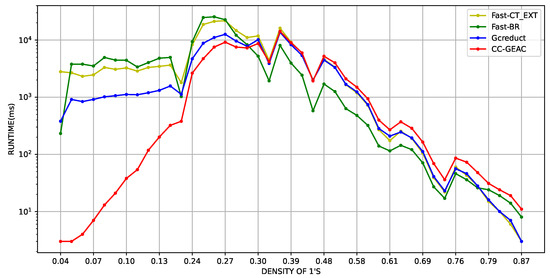
Figure 1.
Average runtime in milliseconds (logarithmic scale) vs. SBDSM’s density, using artificial matrices with 30 columns.
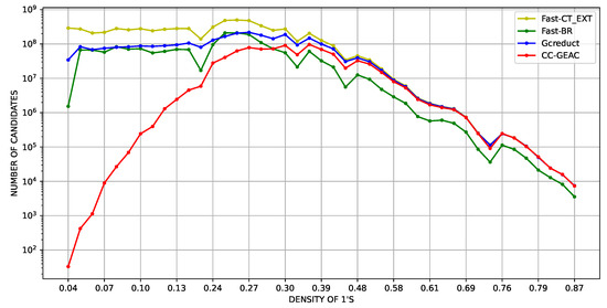
Figure 2.
Average number of evaluated candidates (logarithmic scale) vs. SBDSM’s density, using artificial matrices with 30 columns.
Three distinct Wilcoxon right-tailed tests were performed using 300 matrices with densities less than 0.29 from the 900 artificial SBDSMs containing 30 columns. Each test had a 95% confidence level and an alpha value set at 0.05. The objective was to evaluate the performance of CC-GEAC in computing constructs compared to the Fast-CT_EXT, Fast-BR, and GCreduct algorithms, when each is used for the same purpose with the SBDSM. The results of these tests show a p-value of 0.00 for each test. These results confirm that CC-GEAC is statistically faster than Fast-CT_EXT, Fast-BR, and GCreduct algorithms for computing constructs using SBDSM with a density of less than 0.29.
Furthermore, to delve into the performance of CC-GEAC for SBDSMs with a density of less than 0.29, 300 artificial SBDSMs were generated with 40 columns, and between 40 and 1000 rows. This also allows us to show the behavior of CC-GEAC as long as the number of columns in the SBDSMs increases. Figure 3 and Figure 4 show the average results in the logarithmic scale regarding the runtime and the number of evaluated candidates over artificial SBDSMs with 40 columns. These figures show that our algorithm obtained the best results concerning the runtime and the number of evaluated candidates for artificial SBDSMs with a density of 1’s under 0.29.
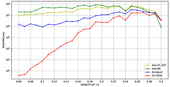
Figure 3.
Average runtime in milliseconds (logarithmic scale) vs. SBDSM’s density, using artificial matrices with 40 columns.
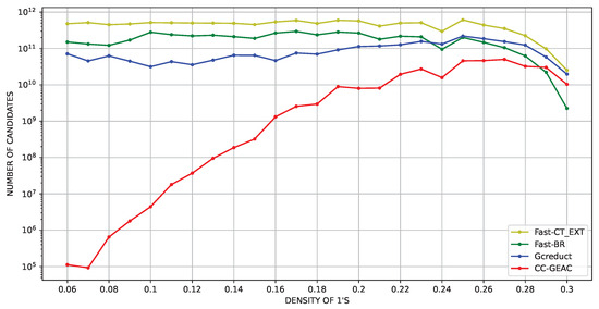
Figure 4.
Average number of evaluated candidates (logarithmic scale) vs. SBDSM’s density, using artificial matrices with 40 columns.
6. Conclusions
As discussed in this paper, the problem of computing constructs has been little studied, with only a few studies proposing methods to compute constructs using algorithms for reducts computation. This paper introduces a new algorithm, CC-GEAC, to compute constructs using the binary simplified discernibility-similarity matrix. Our algorithm utilizes the kernel and the minimum set of attributes to prune the search space, and it searches for gaps in the subsets for further pruning. Additionally, it looks for rows of zeros in the current subset, enabling the elimination of subsets that will never form constructs. We evaluated CC-GEAC and compared it, in terms of runtime and the number of evaluated candidates, against the option of computing constructs using algorithms for reducts computation [8]. Our experiments on real and artificial matrices demonstrate that CC-GEAC is the best option for computing constructs when the discernibility–similarity matrices have densities lower than 0.29. In most cases, our algorithm evaluates fewer attribute subsets than Fast-CT-EXT [11], FastBR [12], and GCreduct [10], which are the fastest state-of-the-art algorithms for reducts computation that can also be used to compute constructs following [8]. However, this efficiency comes at a higher computational cost. Therefore, in future work, we will work on speeding up the process of evaluating candidates. Another line of future work will involve implementing CC-GEAC using GPU-based architectures.
Author Contributions
Y.G.-D., the corresponding author of the contribution “An algorithm for computing all rough set constructs for dimensionality reduction”, hereby confirm on behalf of myself and my co-authors (J.F.M.-T., J.A.C.-O. and M.S.L.-C.) that they have participated sufficiently in the work to take public responsibility for its content. This includes participation in the concept, design, analysis, writing, or revision of the manuscript. Accordingly, the specific contributions made by each author are as follows: J.F.M.-T., J.A.C.-O. and M.S.L.-C.: conceptualization, methodology, reviewing, and editing. Y.G.-D.: investigation, software, data curation, writing—original draft preparation, writing—reviewing and editing. All authors have read and agreed to the published version of the manuscript.
Funding
This research received no external funding.
Data Availability Statement
The datasets used during the current study are available in the “UC Irvine Machine Learning Repository”: https://archive.ics.uci.edu/ml/datasets.php, “OpenML”: https://www.openml.org/; the source code of the CC-GEAC algorithm is available at https://github.com/ygdiaz1202/CC-GEAC.git.
Acknowledgments
The first author thanks the support given by CONAHCYT through his doctoral fellowship.
Conflicts of Interest
The authors declare no conflict of interest.
Abbreviations
The following abbreviations are used in this manuscript:
| RST | rough set theory |
| SAT | Boolean satisfiability problem |
| DS | decision system |
| BDSM | binary discernibility–similarity matrix |
| SBDSM | simplified binary discernibility–similarity matrix |
| MSA | minimum attribute subset |
| CM | cumulative mask |
| CONAHCYT | Consejo Nacional de Humanidades, Ciencias y Tecnologías |
References
- Pawlak, Z. Rough sets. Int. J. Comput. Inf. Sci. 1982, 11, 341–356. [Google Scholar] [CrossRef]
- Susmaga, R. Reducts and constructs in classic and dominance-based rough sets approach. Inf. Sci. 2014, 271, 45–64. [Google Scholar] [CrossRef]
- Kopczynski, M.; Grzes, T. FPGA supported rough set reduct calculation for big datasets. J. Intell. Inf. Syst. 2022, 59, 779–799. [Google Scholar] [CrossRef]
- Bazan, J.G.; Skowron, A.; Synak, P. Dynamic reducts as a tool for extracting laws from decisions tables. In Proceedings of the Methodologies for Intelligent Systems, Charlotte, NC, USA, 16–19 October 1994; Raś, Z.W., Zemankova, M., Eds.; Springer: Berlin/Heidelberg, Germany, 1994; pp. 346–355. [Google Scholar] [CrossRef]
- Stańczyk, U. Application of rough set-based characterisation of attributes in feature selection and reduction. In Advances in Selected Artificial Intelligence Areas: World Outstanding Women in Artificial Intelligence; Springer: Berlin/Heidelberg, Germany, 2022; pp. 35–55. [Google Scholar] [CrossRef]
- Carreira-Perpinán, M.A. A Review of Dimension Reduction Techniques; Technical Report CS-96-09; Department of Computer Science, University of Sheffield: Sheffield, UK, 1997; Volume 9, pp. 1–69. [Google Scholar]
- Susmaga, R.; Słowiński, R. Generation of rough sets reducts and constructs based on inter-class and intra-class information. Fuzzy Sets Syst. 2015, 274, 124–142. [Google Scholar] [CrossRef]
- Lazo-Cortés, M.S.; Carrasco-Ochoa, J.A.; Martínez-Trinidad, J.F.; Sanchez-Diaz, G. Computing constructs by using typical testor algorithms. In Proceedings of the Mexican Conference on Pattern Recognition, Mexico City, Mexico, 24–27 June 2015; Springer: Berlin/Heidelberg, Germany, 2015; pp. 44–53. [Google Scholar] [CrossRef]
- Bao, Y.; Du, X.; Deng, M.; Ishii, N. An efficient method for computing all reducts. Trans. Jpn. Soc. Artif. Intell. 2004, 19, 166–173. [Google Scholar] [CrossRef][Green Version]
- Rodríguez-Diez, V.; Martínez-Trinidad, J.F.; Carrasco-Ochoa, J.A.; Lazo-Cortés, M.S. A new algorithm for reduct computation based on gap elimination and attribute contribution. Inf. Sci. 2018, 435, 111–123. [Google Scholar] [CrossRef]
- Sánchez-Díaz, G.; Piza-Dávila, I.; Lazo-Cortés, M.; Mora-González, M.; Salinas-Luna, J. A fast implementation of the CT_EXT algorithm for the testor property identification. In Proceedings of the Mexican International Conference on Artificial Intelligence, Pachuca, Mexico, 8–13 November 2010; Springer: Berlin/Heidelberg, Germany, 2010; pp. 92–103. [Google Scholar] [CrossRef]
- Lias-Rodriguez, A.; Sanchez-Diaz, G. An algorithm for computing typical testors based on elimination of gaps and reduction of columns. Int. J. Pattern Recognit. Artif. Intell. 2013, 27, 1350022. [Google Scholar] [CrossRef]
- Susmaga, R. Reducts versus constructs: An experimental evaluation. Electron. Notes Theor. Comput. Sci. 2003, 82, 239–250. [Google Scholar] [CrossRef]
- Susmaga, R. Experiments in incremental computation of reducts. Methodol. Appl. 1998. Available online: https://cir.nii.ac.jp/crid/1572824500035732992 (accessed on 1 September 2021).
- Greco, S.; Matarazzo, B.; Slowinski, R. Rough sets theory for multicriteria decision analysis. Eur. J. Oper. Res. 2001, 129, 1–47. [Google Scholar] [CrossRef]
- Martínez-Trinidad, J.F.; Guzman-Arenas, A. The logical combinatorial approach to pattern recognition, an overview through selected works. Pattern Recognit. 2001, 34, 741–751. [Google Scholar] [CrossRef]
- Lazo-Cortés, M.S.; Martínez-Trinidad, J.F.; Carrasco-Ochoa, J.A.; Sanchez-Diaz, G. On the relation between rough set reducts and typical testors. Inf. Sci. 2015, 294, 152–163. [Google Scholar] [CrossRef]
- Felix, R.; Ushio, T. Rough sets-based machine learning using a binary discernibility matrix. In Proceedings of the Second International Conference on Intelligent Processing and Manufacturing of Materials. IPMM’99 (Cat. No.99EX296), Honolulu, HI, USA, 10–15 July 1999; Volume 1, pp. 299–305. [Google Scholar] [CrossRef]
- Skowron, A.; Rauszer, C. The Discernibility Matrices and Functions in Information Systems. In Intelligent Decision Support: Handbook of Applications and Advances of the Rough Sets Theory; Słowiński, R., Ed.; Springer: Dordrecht, The Netherlands, 1992; pp. 331–362. [Google Scholar] [CrossRef]
- Santiesteban Alganza, Y.; Pons Porrata, A. LEX: Un nuevo algoritmo para el cálculo de los testores típicos. Cienc. Mat. 2003, 21, 85–95. [Google Scholar]
- Lias-Rodríguez, A.; Pons-Porrata, A. BR: A new method for computing all typical testors. In Proceedings of the Iberoamerican Congress on Pattern Recognition, Guadalajara, Jalisco, Mexico, 15–18 November 2009; Springer: Berlin/Heidelberg, Germany, 2009; pp. 433–440. [Google Scholar] [CrossRef]
- Piza-Dávila, I.; Sánchez-Díaz, G.; Lazo-Cortés, M.S.; Villalón-Turrubiates, I. An Algorithm for Computing Minimum-Length Irreducible Testors. IEEE Access 2020, 8, 56312–56320. [Google Scholar] [CrossRef]
- Dua, D.; Graff, C. UCI Machine Learning Repository; University of California, School of Information and Computer Science: Irvine, CA, USA, 2019; Available online: http://archive.ics.uci.edu/ml (accessed on 1 September 2021).
- Derrac, J.; Garcia, S.; Sanchez, L.; Herrera, F. Keel data-mining software tool: Data set repository, integration of algorithms and experimental analysis framework. J. Mult. Valued Log. Soft Comput. 2015, 17, 255–287. [Google Scholar]
- Van Rijn, J.N.; Bischl, B.; Torgo, L.; Gao, B.; Umaashankar, V.; Fischer, S.; Winter, P.; Wiswedel, B.; Berthold, M.R.; Vanschoren, J. OpenML: A collaborative science platform. In Proceedings of the Joint European Conference on Machine Learning and Knowledge Discovery in Databases, Prague, Czech Republic, 23–27 September 2013; Springer: Berlin/Heidelberg, Germany, 2013; pp. 645–649. [Google Scholar] [CrossRef]
- Rajalakshmi, A.; Vinodhini, R.; Bibi, K.F. Data Discretization Technique Using WEKA Tool. Int. J. Sci. Eng. Comput. Technol. 2016, 6, 293–298. [Google Scholar]
Disclaimer/Publisher’s Note: The statements, opinions and data contained in all publications are solely those of the individual author(s) and contributor(s) and not of MDPI and/or the editor(s). MDPI and/or the editor(s) disclaim responsibility for any injury to people or property resulting from any ideas, methods, instructions or products referred to in the content. |
© 2023 by the authors. Licensee MDPI, Basel, Switzerland. This article is an open access article distributed under the terms and conditions of the Creative Commons Attribution (CC BY) license (https://creativecommons.org/licenses/by/4.0/).