Finite Difference Models of Dynamical Systems with Quadratic Right-Hand Side

Abstract

Difference schemes that approximate dynamic systems are considered discrete models of the same phenomena that are described by continuous dynamic systems. Difference schemes with t-symmetry and midpoint and trapezoid schemes are considered. It is shown that these schemes are dual to each other, and, from this fact, we derive theorems on the inheritance of quadratic integrals by these schemes (Cooper’s theorem and its dual theorem on the trapezoidal scheme). Using examples of nonlinear oscillators, it is shown that these schemes poses challenges for theoretical research and practical application due to the problem of extra roots: these schemes do not allow one to unambiguously determine the final values from the initial values and vice versa. Therefore, we consider difference schemes in which the transitions from layer to layer in time are carried out using birational transformations (Cremona transformations). Such schemes are called reversible. It is shown that reversible schemes with t-symmetry can be easily constructed for any dynamical system with a quadratic right-hand side. As an example of such a dynamic system, a top fixed at its center of gravity is considered in detail. In this case, the discrete theory repeats the continuous theory completely: (1) the points of the approximate solution lie on some elliptic curve, which at $\Delta t\to 0$ turns into an integral curve; (2) the difference scheme can be represented using quadrature; and (3) the approximate solution can be represented using an elliptic function of a discrete argument. The last section considers the general case. The integral curves are replaced with closures of the orbits of the corresponding Cremona transformation as sets in the projective space over $\mathbb{R}$. The problem of the dimension of this set is discussed.

1. Introduction

Dynamical systems can very rarely be solved analytically, and, therefore, they have to be studied numerically. Currently, the main numerical method of integration is the finite difference method. The general concept of the finite difference method in its application to ordinary differential equations is presented in [1]; the issues associated with conservation of integrals of motion are given a prominent place in [2,3]. Of great importance is the penetration into this theory of ideas and methods that were originally developed for the study of partial differential equations, including the concept of mimetic difference schemes, which inherit, in one sense or another, some properties of the original continuous problem [4,5,6].

The finite difference method proposes replacing the system of differential equations

$$\frac{d{x}_i}{dt}=f_i(x_1,\dots ,x_n),i=1,\dots ,n,$$

or, for short,

$$\frac{d\mathfrak{x}}{dt}=\mathfrak{f}\left(\mathfrak{x}\right),$$

(1)

with a system of algebraic equations

$$g_i(\mathfrak{x},\widehat{\mathfrak{x}},\Delta t)=0,i=1,\dots ,n,$$

(2)

relating the value of the solution at some moment in time t with the value of the solution at the moment in time $t+\Delta t$. In this case, the first value is simply denoted as $\mathfrak{x}$, the second as $\widehat{\mathfrak{x}}$, and the finite value $\Delta t$ is called the time step. The system of the algebraic Equation (2) itself will be called a difference scheme for a system of the differential Equation (1).

The approximate solution of the Cauchy problem

$$\frac{d\mathfrak{x}}{dt}=\mathfrak{f}\left(\mathfrak{x}\right),\mathfrak{x}\left(0\right)={\mathfrak{x}}_0,$$

found using the scheme (2) with a positive step $\Delta t\in \mathbb{R}$, is understood as a sequence of points ${\mathfrak{x}}_0,{\mathfrak{x}}_1,\dots \in {\mathbb{R}}^n$, found recursively, i.e., ${\mathfrak{x}}_{m+1}$ is a solution of

$$g_i({\mathfrak{x}}_m,\widehat{\mathfrak{x}},\Delta t)=0,i=1,\dots ,n,$$

with respect to $\widehat{\mathfrak{x}}$ and closest to $\widehat{\mathfrak{x}}={\mathfrak{x}}_m$. The attention of researchers in the last century was focused on the closeness of ${\mathfrak{x}}_m$ and $\mathfrak{x}(m\Delta t)$.

Setting aside this undoubtedly important mathematical issue, we note that the difference scheme (2) represents a discrete mathematical model of the same phenomenon as the original system of the differential Equation (1). Moreover, in mechanics, both old and new, the quantity $dt$ has often been treated as a finite increment, and it was implied that Newton’s equations were actually difference equations [7]. From this point of view, it seems reasonable that the difference model should be no worse than the differential one. However, the simplest example shows that during discretization the most important properties of a continuous problem are lost.

Consider a linear oscillator

$$\frac{dx}{dt}=-y,\frac{dy}{dt}=x$$

(3)

and the simplest difference scheme for it, the explicit Euler scheme

$$\widehat{x}-x=-y\Delta t,\widehat{y}-y=x\Delta t.$$

(4)

The energy $x^2+y^2$ is conserved in the original differential system, so, in the $xy$ plane, the point moves around a circle with a constant speed. In solutions found using Euler’s scheme, energy is not conserved, and the point $(x,y)$ spirals down to the center of the $xy$ coordinate system instead of spinning in a circle. This contradicts our ideas about oscillations, and this contradiction is removed only in the limit at $\Delta t\to 0$. In fact, when describing the properties of a linear oscillator, we permanently correct our considerations by looking back at the differential formulation, which, therefore, cannot be removed from consideration.

In the general case, the situation remains the same: replacing the differential model with a difference scheme leads to a violation of conservation laws and introduces new phenomena (dissipation or even anti-dissipation), which disappear in the limit $\Delta t\to 0$. This forces us to compare approximate solutions with the exact one all the time.

2. Preservation and Inheritance of Integrals of Motion

In fact, the reasons why the integrals of motion cease to be preserved are not related to the passage to the limit $\Delta t\to 0$. Expression

$$\frac{\overrightarrow{x}(t+\Delta t)-\overrightarrow{x}\left(t\right)}{\Delta t}$$

can be regarded equally well as an approximation to the derivative of the function $\mathfrak{x}$, calculated at any point between t and $t+\Delta t$. By choosing the left end of the segment, we obtain an explicit Euler scheme

$$\frac{\mathfrak{x}(t+\Delta t)-\mathfrak{x}\left(t\right)}{\Delta t}=\dot{\mathfrak{x}}\left(t\right)=\mathfrak{f}\left(\mathfrak{x}\left(t\right)\right).$$

However, with this choice, we violate the original equality of the left and right ends of the considered segment of the t axis, which causes “dissipation”. In the limit $\Delta t\to 0$, this equality is restored and conservation laws appear. It can be assumed that the integrals of motion are preserved in those difference schemes, during the compilation of which the equality of the points t and $t+\Delta t$ is preserved. Let us express this more precisely by formulating two definitions.

Definition 1.

The difference scheme (2) will be said to preserve the expression $h(\mathfrak{x},\Delta t)$ if it follows from Equation (2) that

$$h(\widehat{\mathfrak{x}},dt)=h(\mathfrak{x},\Delta t).$$

If the expression h does not depend on $\Delta t$, then it is an integral of motion of the continuous dynamic system (1). In this case, we will say that the integral of motion h is preserved exactly in the difference scheme. If the expression h depends on $\Delta t$, then the integral of motion will be the limit of this expression when $\Delta t\to 0$. In this case, we will say that this integral is inherited by the difference scheme.

The issue of constructing difference schemes that preserve integrals of motion was studied in the 1990s [2,8]; the issue of conservation of mechanical energy was considered specifically [3,9]. A more subtle concept of inheritance of integrals of motion, presented in Definition 1, came to the theory of dynamical systems from studies of partial differential equations, in which the concept of mimetic difference schemes has been developed [4,5].

Definition 2.

We will say that the difference scheme (2) has t-symmetry if the system of Equation (2) is equivalent to the system

$$g_i(\widehat{\mathfrak{x}},\mathfrak{x},-\Delta t)=0,i=1,\dots ,n.$$

Schemes with t-symmetry are interesting in that they inherit the conservation laws of the original dynamical system. Among the schemes with t-symmetry, we would like to highlight the midpoint scheme

$$\widehat{\mathfrak{x}}-\mathfrak{x}=\mathfrak{f}\left(\frac{\widehat{\mathfrak{x}}+\mathfrak{x}}{2}\right)\Delta t,$$

(5)

and the trapezoid scheme

$$\widehat{\mathfrak{x}}-\mathfrak{x}=\frac{\mathfrak{f}\left(\widehat{\mathfrak{x}}\right)+\mathfrak{f}\left(\mathfrak{x}\right)}{2}\Delta t.$$

(6)

The conservation of integrals in the midpoint scheme was studied in the 1980s by Cooper [2,8].

Theorem 1

(Cooper). The midpoint scheme preserves the linear and quadratic integrals of the dynamical system (1) exactly.

From this theorem, it follows that, e.g., the points of the approximate solution of the linear oscillator (3), found using the midpoint scheme

$$\widehat{x}-x=-(\widehat{y}+y)\frac{\Delta t}{2},\widehat{y}-y=(\widehat{x}+x)\frac{\Delta t}{2}$$

(7)

lie on a circle

$$x^2+y^2=C.$$

(8)

Moreover, in this case, the transition from layer to layer can be described in matrix form

$$\left(\begin{array}{c}\widehat{x}\\ \widehat{y}\end{array}\right)=A\left(\begin{array}{c}x\\ y\end{array}\right),$$

where the transition matrix

$$A=\left(\begin{array}{cc}\frac{4-\Delta t^2}{\Delta t^2+4}& \frac{-4\Delta t}{\Delta t^2+4}\\ \frac{4\Delta t}{\Delta t^2+4}& \frac{4-\Delta t^2}{\Delta t^2+4}\end{array}\right)$$

is a matrix of rotation

$$\left(\begin{array}{cc}cos\Delta \alpha & -sin\Delta \alpha \\ sin\Delta \alpha & cos\Delta \alpha \end{array}\right)$$

by the angle $\Delta \alpha$. Thus, the midpoint scheme allows the linear oscillator model (3) to be discretized so that rotations at equal angles occur over equal periods of time. Qualitatively, the discrete and continuous models are no different; quantitatively, over a time interval $\Delta t$, the continuous model rotates by an angle $\Delta t$, and the discrete model rotates by an angle

$$\Delta \alpha =arcsin\frac{\Delta t}{1+\Delta t^2/4}=\Delta t+\mathcal{O}(\Delta t^3).$$

If, as in the case of a linear oscillator, $\mathfrak{f}$ is a linear function of $\mathfrak{x}$, then

$$\mathfrak{f}\left(\frac{\widehat{\mathfrak{x}}+\mathfrak{x}}{2}\right)=\frac{\mathfrak{f}\left(\widehat{\mathfrak{x}}\right)+\mathfrak{f}\left(\mathfrak{x}\right)}{2},$$

therefore, the trapezoidal scheme (6) will coincide with the midpoint scheme (5). In the nonlinear case, these schemes do not coincide and a natural question arises: are the integrals of motion inherited by the trapezoidal scheme?

To answer this question, note that these two difference schemes are in some sense related to each other. Indeed, let ${\mathfrak{x}}_0,{\mathfrak{x}}_1,{\mathfrak{x}}_2,\dots$ be an approximate solution to Equation (1), calculated using the midpoint scheme (5). Then, the coordinates ${\mathfrak{x}}_0^{\prime },{\mathfrak{x}}_1^{\prime },{\mathfrak{x}}_2^{\prime },\dots$ of the midpoints of the links of the broken line ${\mathfrak{x}}_0{\mathfrak{x}}_1{\mathfrak{x}}_2\dots$ represent another approximate solution to the same equation, calculated using the trapezoidal scheme (6), which was noted in [10]. From this fact, the theorem dual to Cooper’s theorem immediately follows.

Theorem 2

(dual to Cooper’s theorem). If the expression h is preserved in the midpoint scheme (in the sense of Definition 1), then, in the trapezoid diagram, the expression

$$h\left(x-f\left(x\right)\frac{\Delta t}{2}\right)$$

is preserved.

Thus, the linear or quadratic integral of motion h is inherited by the trapezoidal scheme (6), but the expression for the conserved quantity coincides with h only in the limit $\Delta t\to 0$. This circumstance made it difficult to find the integral. We introduced the concept of duality of difference schemes in [10], where a proof of the Theorem 2 can be found as well.

A classical and, at the same time, realistic example of a nonlinear oscillator is offered by a dynamic system that describes the motion of a top fixed at its center of gravity. Although the integration of this model is associated with the names of Euler and Poinsot [11], the movement of the top still causes surprise and interest among those who observe it live. So, for example, there was active discussion on the Internet about wing nut somersaults in zero gravity, which were observed by Janibekov, and which, nevertheless, are perfectly described by this model [12].

Following [11], let us denote the coordinates of the angular velocity vector relative to the principal axes of inertia as $p,q,r$, and the principal moments of inertia as $A,B,C$; then, the angular velocity evolution is described by a dynamic system

$$\dot{p}=aqr,\dot{q}=bpr,\dot{r}=cpq,$$

(9)

the coefficients of which are expressed in terms of the principal moments of inertia

$$a=-\frac{C-B}{A},b=-\frac{A-C}{B},c=-\frac{B-A}{C}.$$

This system has two quadratic integrals

$$A{p}^2+B{q}^2+C{r}^2=C_1\mathrm{and}{A}^2{p}^2+B^2{q}^2+C^2{r}^2=C_2,$$

(10)

which were found back in the 18th century [11]. In the 19th century, they were used to reduce the problem to quadrature and integration in elliptic functions. From the viewpoint of numerical methods, this case is interesting as a nonlinear oscillator with quadratic integrals that are preserved exactly in the midpoint scheme, as noted in [2], and, due to Theorem 2, which is dual to it, the quadratic integrals are inherited in a slightly modified form by the trapezoidal scheme.

In cases in which the integrals of motion are not linear or quadratic, it is still possible to construct difference schemes that preserve all algebraic integrals of motion. One of the simplest ways is the method of quadratizing the integral, which consists of introducing new variables in such a way that, with respect to them, all integrals are linear and quadratic [13,14,15]. In this way, from the midpoint scheme, we were able to construct a difference scheme for the many-body problem, preserving all of its algebraic integrals [16].

There is a large family of schemes, the symplectic Runge–Kutta schemes, which preserve linear and quadratic integrals of the dynamical system [2]. The midpoint scheme discussed above is the simplest of these difference schemes. The dual trapezoidal scheme dual to it does not belong to this family. The integrals of motion in it are not preserved but are inherited in the sense of Definition 1.

3. Implicit Schemes and the Problem of Extra Roots

If $\mathfrak{f}$ is not a linear function of $\mathfrak{x}$, then Equation (5), as well as Equation (6), cease to be linear with respect to $\widehat{\mathfrak{x}}$. This significantly complicates the calculation of approximate solutions: at each step, one has to numerically solve a system of nonlinear algebraic equations, which not only introduces an additional error but also makes calculations using much more laborious schemes than the explicit Euler scheme.

In practice, especially when calculating over long times, they prefer explicit schemes to implicit ones, sacrificing the implementation of conservation laws to the speed of calculations. With a significant violation of conservation laws, of course, even the external similarity of exact and approximate solutions, e.g., trajectories in the many-body problem [16], is lost. The concept of explicit conservative Runge–Kutta schemes was introduced in [17,18]. In fact, these are explicit Runge–Kutta schemes, in which, at each step, the values are corrected so that the specified conservation laws are satisfied [19]. This approach, however, differs significantly from the original finite difference method. It cannot be written using a single difference scheme, which we could interpret as a discrete model of the original dynamical system.

No less problematic is the study of the inheritance of periodicity. We were able to calculate the Gröbner basis of the midpoint scheme for the oscillator and eliminate $\widehat{q},\widehat{r}$ from the system. This leads to the equation

$$f(\widehat{p},p,q,r,\Delta t)=0,$$

having a degree of five with respect to $\widehat{p}$. It is not clear how to investigate it further. Moreover, the physical meaning of the extra roots is not clear: since this is an equation of the fifth order, then, in addition to the desired root $\widehat{p}$, there must be four other roots close to p. Using the explicit form of the polynomial f, it is easy to prove that these roots tend to ∞ as $\Delta t\to 0$. In numerical calculations, this circumstance allows for separation of four extra roots from the fifth one, which is only interesting when calculating an approximate solution.

The question of “extra” roots, surprisingly, has eluded the attention of researchers. Meanwhile, in nonlinear systems they arise naturally.

For example, the explicit Euler scheme

$$\widehat{\mathfrak{x}}=\mathfrak{x}+\mathfrak{f}\left(\mathfrak{x}\right)\Delta t$$

is linear with respect to $\widehat{\mathfrak{x}}$, so a given value of $\mathfrak{x}$ corresponds to one single value $\widehat{\mathfrak{x}}$. However, in the nonlinear case, a given value of $\widehat{\mathfrak{x}}$ corresponds to several values of $\mathfrak{x}$, one of which tends to $\widehat{\mathfrak{x}}$ at $\Delta t\to 0$. These roots are not interesting when finding a numerical solution since we are moving from the ${\mathfrak{x}}_i$ layer to the ${\mathfrak{x}}_{i+1}$ layer, and not vice versa.

The appearance of extra roots in the explicit Euler scheme is not surprising. The surprising thing is that the transition from it to schemes that have t-symmetry and preserve integrals of motion does not lead to the disappearance of extra roots. Their appearance violates another basic principle of mechanics: from the initial data, it should be possible to unambiguously determine the final data and vice versa.

4. Reversible Schemes

It is generally accepted that when constructing difference schemes that inherit the properties of the original differential model, the most important thing is the inheritance of integrals of motion. However, as we saw above, the conservation of integrals and t-symmetry does not rid the scheme of the extra roots discussed in the previous section. The desire to get rid of them led us to a difference scheme in which a given initial value $\mathfrak{x}$ corresponds to one single final value $\widehat{\mathfrak{x}}$, and a given final value $\widehat{\mathfrak{x}}$ to one initial value $\mathfrak{x}$. In [20], we proposed calling such difference schemes reversible.

The described construction is well known in algebraic geometry [21]. We call a difference scheme reversible if its equations define a birational transformation between those varieties whose points are $\mathfrak{x}$ and $\widehat{\mathfrak{x}}$.

The question of choosing these varieties is not trivial, but, for now, we will consider the simplest option when the difference scheme specifies a birational transformation between an n-dimensional $\mathfrak{x}$-space and an n-dimensional $\widehat{\mathfrak{x}}$-space, i.e., the Cremona transformation [21]. Only for such a difference scheme will we retain the name reversible.

Reversible schemes may seem very rare, but, in reality, for any dynamical system with a quadratic right-hand side, we have such a reversible scheme

$$\widehat{\mathfrak{x}}-\mathfrak{x}=\mathfrak{F}\Delta t,$$

where the right-hand side $\mathfrak{F}$ is obtained from the right-hand side $\mathfrak{f}$ of the original dynamical system by replacing the squares $x_i^2$ with $x_i{\widehat{x}}_i$ and the mixed terms $x_i{x}_j$ with $\frac{1}{2}({\widehat{x}}_i{x}_j+x_i{\widehat{x}}_j)$; see [20].

It should be noted that the class of dynamical systems with a quadratic right-hand side is very wide. This includes, for example, equations describing the motion of a rigid body, which can be studied by analytical methods only in three special cases [11]. Moreover, by virtue of Appelroth’s theorem [22], any dynamical system can be reduced by an appropriate algebraic substitution to a system with a quadratic right-hand side. For polynomial systems, software are available to perform such quadratization [23].

In the theory of dynamical systems, discrete systems in which the step is described by the Cremona transformation were considered by A.P. Veselov [24], and special examples were considered by Henon and Moser [25]. Example 3 in [24] leaves no doubt that A.P. Veselov considered the possibility of obtaining such discrete models from continuous ones; however, these authors restricted their consideration to Cremona polynomial transformations. The above method of discretizing a dynamical system with a quadratic right-hand side inevitably leads to Cremona transformations that are not polynomial.

When calculating an approximate solution using a reversible difference scheme, at each step, it is necessary to solve a system of linear equations. This makes calculations using such schemes much simpler than similar calculations using implicit Runge–Kutta schemes, where, recall, at each step, it is necessary to solve a system of nonlinear equations. The complexity of calculations using reversible schemes is close to the complexity of calculations using explicit conservative second-order Runge–Kutta schemes. Let us show with examples that, in this case, reversible schemes inherit the properties of the original continuous models.

5. Motion of a Top in the Euler–Poinsot Case

Among continuous dynamic models with a quadratic right-hand side, the oscillators that are integrable in elliptic functions deserve special attention. In Ref. [20], we considered several such oscillators, including the Jacobi and Weierstrass ones. Both of these cases can be considered a kind of variation in the dynamical system that describes the motion of the top in the Euler–Poinsot case and is integrable in elliptic functions. Traditionally, the Euler–Poinsot case is reduced to the Jacobi oscillator [11], but, in fact, the properties of the reversible difference scheme for a top are conveniently described in the original coordinates. For a top fixed at the center of gravity, it is not difficult to construct, without any substitutions, a reversible and t-symmetric difference scheme that approximates the system of the differential Equation (9):

$$\widehat{p}-p=(\widehat{q}+q)(\widehat{r}+r)\frac{a\Delta t}{4},\dots$$

(11)

Elliptic oscillators were the subject of intense study in the 19th century, so their analytical properties are well known [26]. This makes them a very convenient test when studying difference schemes and, especially, when studying the question of whether difference schemes inherit the properties of the original continuous problem.

5.1. Integral Curves

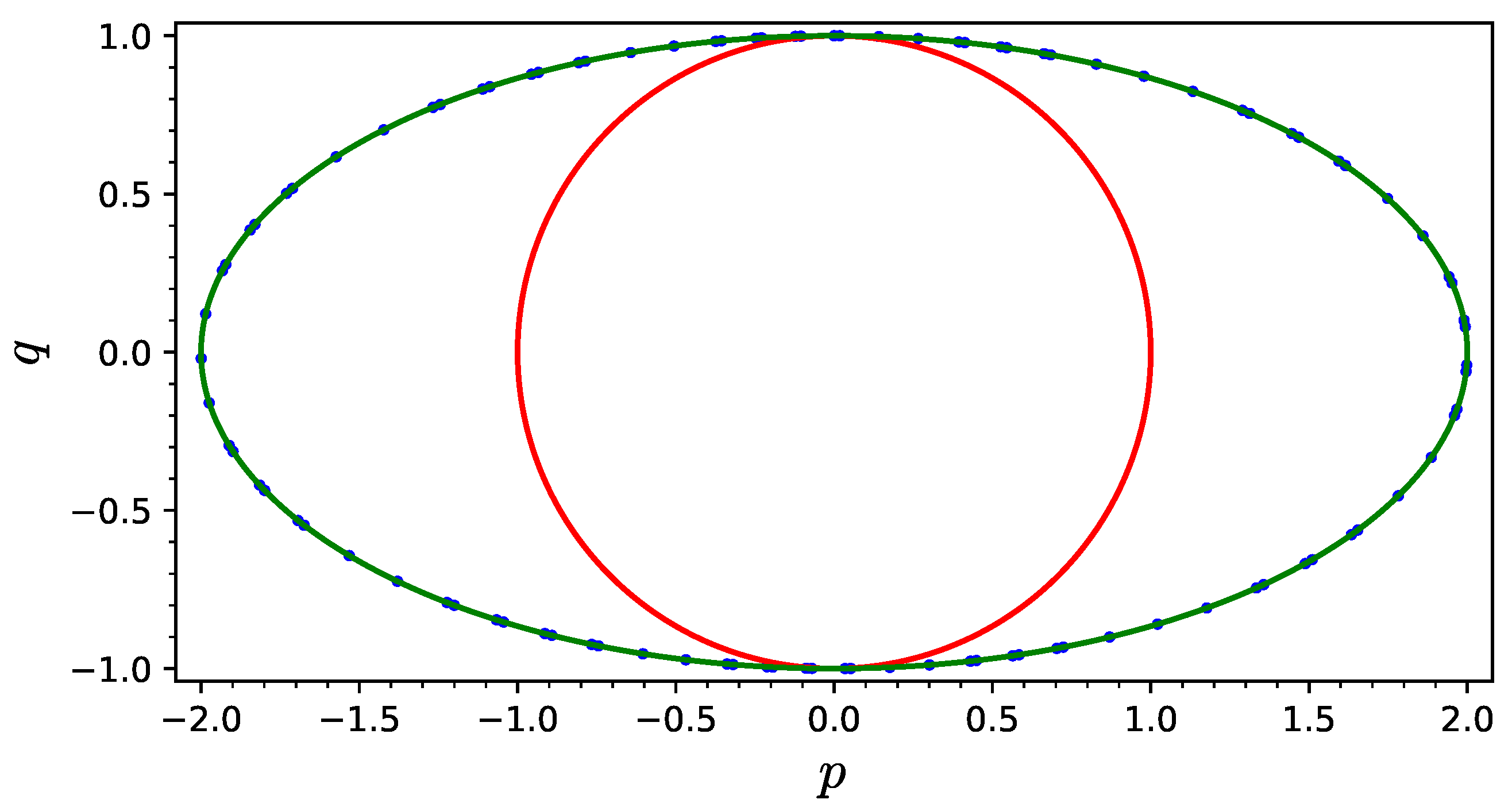
Carrying out numerical experiments with this scheme, we noticed that the points of the approximate solution line up along a curve resembling an ellipse but are noticeably different from the integral curve. In Figure 1, the integral curve and the ellipse on which the points of the approximate solution lie are shown.

To create an equation for the curve on which the points of the approximate solution lie, we had to extend the Lagutinski theory [27,28,29] to the finite difference case [30].

Theorem 3.

Let a linear system of the form

$$\sum _{i=0}^m{a}_i{g}_i\left(\mathfrak{x}\right)=0,$$

(12)

be given, where $a_0,\dots ,a_m$ are numerical parameters from $\mathbb{R}$. If, for any approximate trajectory ${\mathfrak{x}}_0,{\mathfrak{x}}_1,\dots$ of system (1), the Cremona determinant

$$det\left(g_i\left({\mathfrak{x}}_j\right)\right)=0(i,j=0.1,\dots m),$$

(13)

is equal to zero, then the approximate trajectories lie on the hypersurfaces of system (12).

From Figure 1, it is easy to find that the projection of the solution points onto the $pq$ plane lies on the ellipse of the linear family

$$a_1{p}^2+a_2{q}^2+a_3=0.$$

(14)

To prove this rigorously, it is enough to consider the coordinates of the initial point ${\mathfrak{x}}_0$ as symbolic variables, calculate the coordinates of the points ${\mathfrak{x}}_1$ and ${\mathfrak{x}}_2$ in symbolic form, and then calculate determinant (13). These calculations can be completed in Sage without any noticeable expenditure of time. The determinant turned out to be equal to zero, so the projections of the solution points onto the $pq$ plane lie on the ellipse of linear family (14).

The equation itself is not difficult to find: Just replace the last line in the determinant with $p^2,q^2,1$. After the reduction in unimportant factors, we arrive at the equation

$$abc\Delta t^2{p}_0^2{q}^2-abc\Delta t^2{p}^2{q}_0^2+4b{p}^2-4b{p}_0^2-4a{q}^2+4a{q}_0^2=0.$$

(15)

Let us transform this equation into the form

$$\frac{b(4-ac\Delta t^2{q}_0^2)}{4b{p}_0^2-4a{q}_0^2}{p}^2-\frac{a(4-bc\Delta t^2{p}_0^2)}{4b{p}_0^2-4a{q}_0^2}{q}^2=1.$$

Assuming that

$$C=\frac{4-ac\Delta t^2{q}_0^2}{4b{p}_0^2-4a{q}_0^2},$$

we have

$$bC{p}^2-a\left(C-\frac{c\Delta t^2}{4}\right)q^2=1.$$

(16)

Thus, the projections of the points of the approximate solution lie on curves belonging to the same pencil (16). In other words, the approximate solution retains the expression

$$\frac{b{p}^2-a{q}^2}{1+\frac{c\Delta t^2}{4}a{q}^2}=\mathrm{const}$$

(17)

in the sense of Definition 1. This expression at $\Delta t\to 0$ transforms into the integral $b{p}^2-a{q}^2=C$ of the initial system.

Similarly, we can study the projection onto the $pr$ plane and arrive at the following theorem.

Theorem 4.

The points of the approximate solution of system (9), found using the reversible scheme (11), lie on the curve

$$\frac{b{p}^2-a{q}^2}{1+\frac{c\Delta t^2}{4}a{q}^2}=C_1,\frac{c{p}^2-a{r}^2}{1+\frac{b\Delta t^2}{4}a{r}^2}=C_2,$$

(18)

where $C_1,C_2$ are appropriately chosen constants.

5.2. Representation of a Difference Scheme in the Form of a Quadrature

Curve (18) is an elliptic curve, similar to the integral curve in the continuous case. This curve is invariant under the Cremona transformation, which is defined by the difference scheme (11). Therefore, the narrowing of this transformation to a transformation on curve (18) is birational. Birational transformations on an elliptic curve can always be described using Abelian integrals of the first type [21,31].

Consider a differential

$$\frac{dp}{qr}$$

on curve (18). Expressing $q,r$ in terms of p by means of Equation (18), we can transform it to the form

$$\frac{dp}{\sqrt{f_4\left(p\right)}},$$

up to the choice of the root branch, where $f_4$ is a polynomial of a degree of four with simple roots. This expression has integrable singularities everywhere [32] and, therefore, is a differential of the first kind.

Theorem 5.

The points of the approximate solution of system (9), found by means of the reversible scheme (11), satisfy the relation

$$\underset{{\mathfrak{x}}_n}{\overset{{\mathfrak{x}}_{n+1}}{\int }}\frac{dp}{qr}=\Delta u,$$

(19)

where $\Delta u$ depends on $\Delta t$ and the initial data, and the integral is considered an Abelian integral on curve (18).

Proof. 

Let O be an arbitrary point of the space $pqr$ and $\widehat{x}=\mathfrak{R}(\mathfrak{x},\Delta t)$. The expression

$$\underset{O}{\overset{\mathfrak{R}(\mathfrak{x},\Delta t)}{\int }}\frac{dp}{qr}$$

as a function of $\mathfrak{x}$ is also an integral of the first kind; therefore, there exist such f and g that

$$\underset{O}{\overset{\mathfrak{R}(\mathfrak{x},\Delta t)}{\int }}\frac{dp}{qr}=f(\Delta t)\underset{O}{\overset{\mathfrak{x}}{\int }}\frac{dp}{qr}+g(\Delta t).$$

(20)

Let us make point $\mathfrak{x}$ pass a closed loop. In this case, there exist such integers $n,m$, that

$$f(\Delta t)\omega =n\omega +m{\omega }^{\prime },$$

where $\omega ,{\omega }^{\prime }$ are fundamental periods of curve (18), which, generally, depend on $\Delta t$. For $\Delta t\to 0$, the image of $\mathfrak{x}$ tends to $\mathfrak{x}$; therefore, $f\left(0\right)=1$, $n=1$, and $m=0$. However, function f cannot change discretely, while m and n, on the contrary, take only integer values. Therefore, it is valid that $n=1$ and $m=0$ not only at $\Delta t=0$ but also at other values of $\Delta t$. Therefore,

$$f(\Delta t)=1.$$

Hence, (20) can be rewritten in the form

$$\underset{\mathfrak{x}}{\overset{\widehat{\mathfrak{x}}}{\int }}\frac{dp}{qr}=g(\Delta t),$$

from which (19) immediately follows. □

The analogue of relation (19) in the continuous case is well known. On the integral curve, the equation

$$\frac{dp}{dt}=aqr$$

can be rewritten in the form of the so-called quadrature

$$\int \frac{dp}{qr}=at,$$

where, on the left, $q,r$ are considered functions of p. In particular, it follows that

$$\underset{\mathfrak{x}\left(t_n\right)}{\overset{\mathfrak{x}\left(t_{n+1}\right)}{\int }}\frac{dp}{qr}=a\Delta t.$$

Therefore, the representation of an approximate solution in the form of (19) will be called a quadrature.

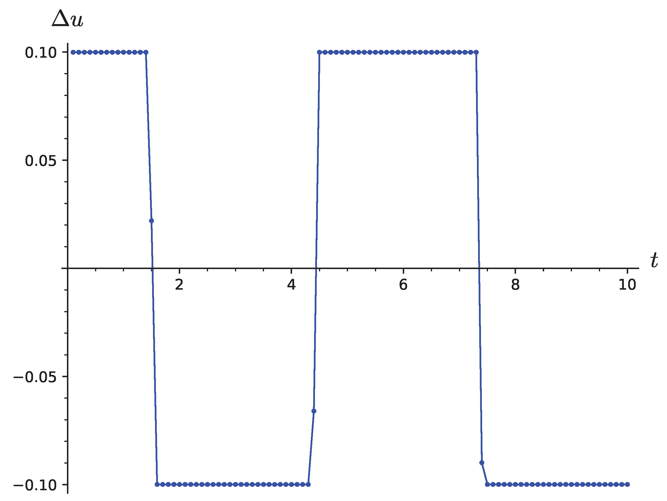
When applying Equation (19), the choice of root must be taken into account. If we agree to choose the arithmetic value of the root, then the value of $\Delta u$ remains constant at almost all steps, except for those during which the branch of the root should be changed. In Figure 2, the usual form of the dependence of $\Delta u$ on the time is presented. It is clearly seen that $\Delta u$ takes two values that differ in sign. Switching between these values does not occur abruptly but, rather, in one or two steps.

In continuous theory, quadratures arise due to the fact that a separation of variables can be performed on the integral curve. The appearance of quadratures in discrete theory cannot be but a surprise.

The transition from ${\mathfrak{x}}_0$ to ${\mathfrak{x}}_m$ using a difference scheme requires the calculation of intermediate positions ${\mathfrak{x}}_1,\dots ,{\mathfrak{x}}_{m-1}$. Representing the difference scheme as a quadrature allows us to describe the transition from ${\mathfrak{x}}_0$ to ${\mathfrak{x}}_m$ without these intermediate steps. This is important not so much for practical calculations—the numerical calculation of the quadrature will still require cutting the integration segment into columns—but for studying the periodicity of the approximate solution.

5.3. Periodicity of Approximate Solution

Since the points of the approximate solution lie on closed curves, the motion remains periodic in the discrete case. It seems quite natural to take as a definition that an approximate solution that is a periodic sequence of points in an affine space is periodic. However, usually the period is a value that is not comparable with the step $\Delta t$. To circumvent this difficulty, we will adopt the following definition.

Definition 3.

We will say that the approximate solution ${\mathfrak{x}}_0,{\mathfrak{x}}_1,\dots$ is periodic with period T if there exists a number $\Delta u$ and a smooth T-periodic function g such that

$${\mathfrak{x}}_m=g(m\Delta u).$$

Let us prove that the approximate solutions found using the reversible scheme are periodic in this sense. Quadrature is an additive function of integration points, so, from (19), it follows that

$$\underset{{\mathfrak{x}}_0}{\overset{{\mathfrak{x}}_m}{\int }}\frac{dp}{qr}=m\Delta u.$$

Since the integral curve (18) is elliptic, and $dp/qr$ is a differential of the first kind, there exists a meromorphic function ℘ such that

$${\mathfrak{x}}_m=\wp (m\Delta u).$$

Since an elliptic interval has a pair of incommensurable periods, this meromorphic function is doubly periodic. Thus, the motion in both the continuous and discrete top models is described by elliptic functions.

Since the zeros of the polynomial $f_4$ are real, one of the periods of the function ℘ is real, and the second is imaginary. The above is true for both continuous and discrete cases. Only in the discrete case do the periods depend on $\Delta t$. Thus, ℘ is a smooth function having a real period T depending on $\Delta t$. Thus, all conditions for Definition 3 are satisfied, and any approximate solution to problem (9) found using a reversible scheme can be considered periodic. This is extremely important since periodicity is the most important and most noticeable of all the qualitative properties of a function.

Thus, in this case, the reversible difference scheme imitates all the known properties of the indispensable model of a top fixed at its center of gravity. The main difference is that, in the discrete case, the transition from layer to layer is carried out by the Cremona transformation of the entire $pqr$ space and, in the continuous case, by a birational transformation on the integral curve. From this point of view, the discrete model is simpler than the continuous one.

There are a number of examples of dynamical systems with a quadratic right-hand side whose integral curves are algebraic curves. All of them, of course, were reduced to quadratures back in the 19th century and, in this sense, were solved analytically. If an invertible difference scheme inherits the algebraic integrals of the original system, then it specifies a birational correspondence on the algebraic curve, the connection of which, with integrals of the first type [21], inevitably leads to the representation of the difference scheme in the form of a quadrature. The integral curves of the classical nonlinear Jacobi and Weierstrass oscillators, as well as system (9) considered above, are elliptic curves. They are inherited by a reversible difference scheme, and, in all these cases, the difference scheme can be described in the form of a quadrature.

6. Approximate Trajectories in Projective Spaces

Turning again to the general case of a dynamical system with a quadratic right-hand side, we note that the transition from layer to layer is given by rational functions, the denominators of which, generally speaking, can turn into zero. In the case of the top, discussed in the last section, we are not faced with such a situation, so there was no need to move to a projective space. However, the simplest mathematical models lead to the appearance of points at infinity.

Consider, for example, the Riccati equation

$$\frac{dp}{dt}=1+p^2,$$

(21)

the solution of which, under the initial condition $p\left(0\right)=0$, is $p=tant$. This solution goes to infinity at $t=\frac{\pi }{2}+\pi n$, $n\in \mathbb{Z}$. An approximate solution found using a reversible scheme with a deliberately large step is presented in Figure 3. It imitates this departure to infinity, correctly describing the behavior of the solution not only before the first pole but also after it. This amazing property of reversible schemes was noted in [33]. The property is also preserved for nonlinear oscillators, for example, the ℘-oscillator

$$\frac{d^{2}p}{d{t}^2}=a{p}^2+bp+c,$$

the exact solution of which also periodically goes to infinity [20].

The appearance of a singular point in the considered interval has a fatal effect on the applicability of the Euler scheme [34]. It was only in the late 2000s that it was realized that this was a problem with the Euler and related schemes. However, the finite difference method itself can be used to determine the position of moving singular points [35,36]. Examples show that reversible difference schemes correctly describe the solution going to infinity and returning.

By default, for the dynamical systems (1), the position of the system $\mathfrak{x}$ is considered a point in the affine space. Now we have an obvious reason to expand the space under consideration to projective space by adding a hyperplane at infinity. This is a natural extension for the study of Cremona transformations [21]. In analytical theory [37] (chapter 4), when studying the Riccati equation, they switched from the affine line to the projective line in the second half of the 19th century.

Thus, we consider $\mathfrak{x}$ as a point in the projective space ${\mathbb{P}}_n$, and the discrete model of the dynamical system (1) as a transition from layer to layer:

$$\widehat{\mathfrak{x}}=C\mathfrak{x},$$

described by the Cremona transformation C depending on $\Delta t$.

When calculating an approximate solution that takes the value ${\mathfrak{x}}_0$ at $t=0$, we calculate the points in the sequence $\left\{{\mathfrak{x}}_n\right\}$ recursively using the formula

$${\mathfrak{x}}_{k+1}=C{\mathfrak{x}}_k.$$

If at some value k the denominator of the transformation becomes zero, then the point ${\mathfrak{x}}_{k+1}$ will be infinitely remote. Such an interpretation is impossible only in one case when both the denominator and all numerators turn to zero. Such points are known as singular points of the Cremona transformation.

One problem arises here that is specific to multidimensional Cremona transformations: a singular point can transform into a line [21]. For example, the Cremona transformation

$$\widehat{x}=\frac{1}{x}=\frac{y}{xy},\widehat{y}=\frac{x}{y}=\frac{x^2}{xy}$$

has a singular point at zero $(0,0)$. The limit

$$\underset{(x,y)\to (0,0)}{lim}\frac{x}{y}$$

is indeterminate and by the transformation the point $(0,0)$ (or its vicinity) “spreads” into a straight line $x=\infty$ at infinity. We can sublate the uncertainty of the limit by directing the point to zero not in an arbitrary manner, but along a certain line.

When calculating an approximate solution, this line is determined in a natural way. Let us assume that ${\mathfrak{x}}_m$ is not a singular point, but ${\mathfrak{x}}_{m+1}=C{\mathfrak{x}}_m$ is, and, formally, we cannot define $C^2{\mathfrak{x}}_m$. Let the point $\mathfrak{x}$ move along the segment ${\mathfrak{x}}_m{\mathfrak{x}}_{m+1}$ to $\mathfrak{x}={\mathfrak{x}}_{m+1}$, then $C\mathfrak{x}$ moves to some position, which we will take to be ${\mathfrak{x}}_{m+2}$. Having accepted this convention, we can regard the approximate solution either as an infinite sequence or as consisting of one singular point, unsuccessfully taken as the initial one.

The process of calculating an approximate solution can be continued towards negative values of m by adopting a similar convention of continuation through singular points. Thus, below, by the approximate solution released from the point $\mathfrak{x}$, we mean the sequence

$$O\left(\mathfrak{x}\right)=\{C^m\mathfrak{x},m\in \mathbb{Z}\},$$

i.e., the orbit of transformation C. This sequence, under the accepted assumptions, is defined for all $\mathfrak{x}\in {\mathbb{P}}_n$, except for a finite number of singular points of transformation C.

7. Closure of the Approximate Trajectory

Let us denote the closure of the set $O\left(\mathfrak{x}\right)$ in ${\mathbb{P}}_n$ by $Z\left(\mathfrak{x}\right)$. This set is obviously invariant under the transformation C. The equality $Z\left(\mathfrak{x}\right)=Z\left({\mathfrak{x}}^{\prime }\right)$ means that the different integral curves $O\left(\mathfrak{x}\right)$ and $O\left({\mathfrak{x}}^{\prime }\right)$ are close to each other, and, therefore, they should not be distinguished.

In the case of the top in (9), the set $Z\left(\mathfrak{x}\right)$ is either a finite set (when $O\left({\mathfrak{x}}_0\right)$ is a periodic sequence) or an elliptic curve (18) in the space $pqr$. It is interesting to note that if we choose the coordinates of the point ${\mathfrak{x}}_0$ and the step $\Delta t$ as rational numbers, we will obtain an infinite sequence of rational points $O\left(\mathfrak{x}\right)$ on the elliptic curve (18), which has been the subject of many studies [38].

Let us take a point ${\mathfrak{x}}^{\prime }\in Z\left(\mathfrak{x}\right)$ that does not belong to $O\left(\mathfrak{x}\right)$. Due to the invariance of $Z\left(\mathfrak{x}\right)$, the orbit $O\left(\mathfrak{x}\right)$ belongs entirely to $Z\left(\mathfrak{x}\right)$. In the case of the top at $\Delta t\to 0$, the curve $Z\left(\mathfrak{x}\right)$ becomes an exact integral curve, so $O\left(\mathfrak{x}\right)$ and $O\left({\mathfrak{x}}^{\prime }\right)$ can be interpreted as “approximations” to the same exact solution.

However, as soon as we slightly shift the center of a top’s fixation from the center of gravity, the situation changes radically. The points of the approximate solution cease to line up along a certain curve. First of all, the dimension of the system itself changes from three to six unknown functions, which are usually taken as $p,q,r$ and direction cosines of the moving axis $Oz$ [11]. This dynamical system has a quadratic right-hand side, and, using the above method, it is possible to construct a reversible difference scheme for it.

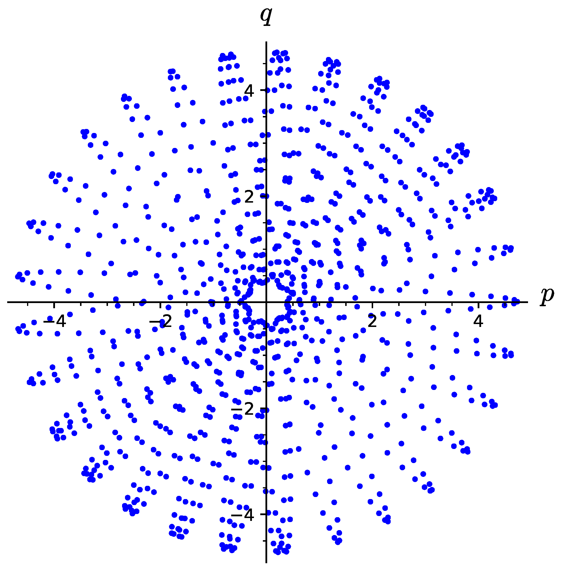
In the case of a symmetric top ($A=B$, Lagrange–Poisson case [11,39]), the projection of a particular solution into the space $pqr$ lies on the plane $r=C$, and the trajectory densely fills some ring on this plane. Computer experiments (see Figure 4) indicate that this property is inherited by the approximate solution found using a reversible scheme. Thus, $Z\left(\mathfrak{x}\right)$ can be a piece of the two-dimensional variety. In the case of an asymmetric top, we have no analytical description of the exact solution. Experiments with a reversible difference scheme suggest that, in the asymmetric case, the set $Z\left(\mathfrak{x}\right)$ is a surface that, at $A-B\to 0$, “collapses” into a ring.

Initially, we believed that all properties of a discrete model could be studied using algebraic methods. However, now we see that the study of the properties of solutions found using reversible schemes is, to a large extent, the study of the set $Z\left(\mathfrak{x}\right)$. In simple cases (for example, in those considered in Section 5), this set turns out to be an algebraic curve, and, therefore, the approximate solutions turn out to be periodic. In more complex cases, this set is neither algebraic nor one-dimensional. Currently, there are no methods at our disposal for calculating the dimension of $Z\left(\mathfrak{x}\right)$; we cannot even rule out that this dimension may be fractal [40]. In all the examples that we have examined in computer experiments, it seemed that the points either lined up in some lines or lay on some surfaces. However, this cannot serve as proof that the dimension of this set is always an integer. The appearance of such a complex object in discrete theory is due to the fact that a reversible difference scheme can be constructed for any dynamical system with a quadratic right-hand side (Section 4).

8. Conclusions

In this paper, we considered difference schemes that approximate dynamic systems as discrete models of the same phenomena that describe continuous dynamical systems. The key problem facing this view seems to be the violation of fundamental conservation laws (Section 2). However, it soon becomes clear (Section 3) that conservative schemes are very difficult to study. Instead of conservatism, we based our approach on reversibility: we consider difference schemes in which the transition from layer to layer in time is carried out using Cremona transformations. Such difference schemes can be constructed for all dynamical systems with a quadratic right-hand side (Section 4).

Among these systems, the one that describes the motion of a top fixed at its center of gravity is distinguished. In this case, the discrete theory repeats the continuous theory completely up to the appearance of integral curves (Section 5.1) and the representation of the solution in the form of elliptic functions (Section 5.3). In fact, we can construct the entire theory of elliptic functions as a branch of the theory of invertible difference schemes.

This theory shows that approximate solutions can be interpreted as periodic in the sense of Definition 3. This allows us to raise the question of finding solutions that are periodic in this sense in other cases and take a fresh look at the already classical problem of finding partial periodic solutions of a particular dynamical system, for example, the many-body problem.

In the general case, the place of integral curves is taken by the closures of the orbits of the corresponding Cremona transformation. These closures, discussed in the last section, are curves in the case of a top fixed at its center of gravity, and, in the general case, their dimension can be greater.

In practice, it is impossible to distinguish between solutions lying on the same closure Z since their trajectories approach each other arbitrarily closely. In our theory, what is of interest is not a separate integral curve calculated using one or another difference scheme, but rather the closure of the set of its points in projective space. This creates the main difficulty in our theory since the closure, as we found out in the examples, is not always a curve or at least an algebraic set. Essentially, it is here that the transcendental penetrates the purely algebraic theory of invertible difference schemes.

This opens up two avenues for us to research further. Following the authors of the 19th century, we can identify and classify systems in which the closure $Z\left(\mathfrak{x}\right)$ is structured quite simply. It is quite obvious that we should start with the case in which $Z\left(\mathfrak{x}\right)$ are curves of genus 0, 1, or greater. The second way is to conduct computer experiments. Unlike the authors of the 19th century, we can always calculate arbitrarily many points $Z\left(\mathfrak{x}\right)$ and try to estimate the dimension of this set. We believe that, over time, it will be possible to replace the non-integrability of a system with a description of specific properties of the sets $Z\left(\mathfrak{x}\right)$. We believe that reversible difference schemes can add a constructive element to the analytical studies of systems that have not yet been integrated.